

Abstract
Most current methods for detecting natural selection from DNA sequence data are limited in that they are either based on summary statistics or a composite likelihood, and as a consequence, do not make full use of the information available in DNA sequence data. We here present a new importance sampling approach for approximating the full likelihood function for the selection coefficient. The method treats the ancestral recombination graph (ARG) as a latent variable that is integrated out using previously published Markov Chain Monte Carlo (MCMC) methods. The method can be used for detecting selection, estimating selection coefficients, testing models of changes in the strength of selection, estimating the time of the start of a selective sweep, and for inferring the allele frequency trajectory of a selected or neutral allele. We perform extensive simulations to evaluate the method and show that it uniformly improves power to detect selection compared to current popular methods such as nSL and SDS, under various demographic models and can provide reliable inferences of allele frequency trajectories under many conditions. We also explore the potential of our method to detect extremely recent changes in the strength of selection. We use the method to infer the past allele frequency trajectory for a lactase persistence SNP (MCM6) in Europeans. We also study a set of 11 pigmentation-associated variants. Several genes show evidence of strong selection particularly within the last 5,000 years, including ASIP, KITLG, and TYR. However, selection on OCA2/HERC2 seems to be much older and, in contrast to previous claims, we find no evidence of selection on TYRP1.
Author summary Current methods to study natural selection using modern population genomic data are limited in their power and flexibility. Here, we present a new method to infer natural selection that builds on recent methodological advances in estimating genome-wide genealogies. By using importance sampling we are able to efficiently estimate the likelihood function of the selection coefficient. We show our method improves power to test for selection over competing methods across a diverse range of scenarios, and also accurately infers the selection coefficient. We also demonstrate a novel capability of our model, using it to infer the allele’s frequency over time. We validate these results with a study of a lactase persistence SNP in Europeans, and also study a set of 11 pigmentation-associated variants.
Introduction
Direct observation of the change in allele frequency over time (the allele frequency trajectory) allows one to make powerful inferences regarding whether selection acted on the allele [1, 2]. However, outside of certain contexts such as experimental evolution of viruses or bacteria [3–6] or analyses of ancient DNA samples [7, 8], in most cases such direct observations of allele frequencies at multiple points in the history of a population are unavailable. Instead, selection must be inferred from contemporary, modern data. A wide variety of methods have been developed to detect selection based on patterns observed from modern DNA sequences (e.g. [9–11]).
The hitch-hiking effect provides a key signature of selection in modern datasets [12]. [12, 13]. Hitch-hiking causes aberrations in the spatial pattern of genetic diversity, including the site frequency spectrum (SFS) [14, 15] and the pattern of haplotype homozygosity [9]. Methods designed to detect these aberrations are particularly useful in the setting where a single population is surveyed, and the only information available is variation within this single population.
The most familiar methods for detecting selection are based on linear functionals of the SFS, such as Tajima’s D, Fu and Li’s D, or Fay and Wu’s H [14, 16, 17]. An advantage of SFS-based methods is that they do not require the data to be phased. However, these methods have several limitations: they tend to confound selection with other non-equilibrium conditions, such as a fluctuating population size [10, 18]; they are not suitable for estimating parameters such as the value of the selection coefficient s; significance can usually only be established using an empirical null distribution; and crucially, these methods do not incorporate any features of the haplotype structure.
To make fuller use of information provided by phased sequence data, a number of methods have incorporated summary statistics based on haplotype structure. In a broad sense, these methods are based on calculations of haplotype similarity in a window around some core site of interest [9]. Several methods have adapted this general concept to specifically detect ongoing selection [11, 19, 20]. More recently, [21] showed that the density of singletons surrounding a focal SNP can be a powerful signal of extremely recent selection in large cohorts. In addition to recent and ongoing selection, it has been demonstrated that these methods have compelling advantages to detecting selection from standing variation [20–22]. However, these methods share the major limitation of SFS-based method in that they are not suitable for parametric inference and it is unclear how to establish significance without use of an empirical null model.
Recently, supervised machine learning methods have been proposed as an alternative to traditional summary-statistic based methods (see e.g., [23]). Standard machine learning techniques applied to population genomic data afford some major advantages over methods based on summary-statistics: standard techniques can produce accurate classifiers based on summaries of the data that live in much higher-dimensional space than the aforementioned summary statistics, and these techniques often encompass a wide space of classification functions that are often non-linear (see e.g. [24, 25]). Some studies have demonstrated these methods can have improved robustness to demographic model mis-specification [22, 26]. Although these methods can potentially detect complex patterns left by selection, they accordingly demand a great deal more training data or otherwise risk overfitting.
In contrast to the aforementioned methods, one might aim to develop a full likelihood methods which would take into account the full data set, rather than merely summary statistics. A common strategy for obtaining the full likelihood has been to find the distribution of the genealogy under selection. For example, Krone and Neuhauser described the distribution of the coalescence tree of a locus under weak selection and no recombination [27]. Alternatively, one can describe how the genealogy depends on the trajectory of the selected allele (first described by [28]), and in turn how the trajectory depends on selection. To this end, Coop and Griffiths [29] developed a sampling method for approximating the full likelihood of the selection coefficient. Their method uses sampling to marginalize out two layers of latent variables: the allele frequency trajectory and the genealogy of the locus. To estimate the likelihood function, they perform random sampling of both the trajectory, and the genealogy conditioned on the trajectory. Unfortunately, methods that consider the both coalescence and recombination are generally considered computationally intractable.
Composite likelihood methods (see e.g. [10, 30]) are able to approximate the likelihood function using tractable expressions for the frequency distribution of a neutral site linked to the selected site [15, 31]. These methods approximate the joint distribution of frequencies observed at linked sites as the product of their marginals. These approaches can be applied to test for selection, and estimate the strength of selection. The approximations made by composite likelihood methods are more accurate under strong selection (arguably beyond the strength of most recent selection in humans), and thus have less power to detect weak selection — although to some extent low power to detect weak selection is a natural outcome of any selection method.
Approximate Bayesian computation (ABC) and rejection sampling methods approximate the likelihood function by simulation. One advantage over the composite likelihood approach is that ABC can capture dependencies between linked neutral sites. For example, methods have been used to jointly infer the strength and timing of selection acting on a locus and determine whether a sweep occurred from a de novo vs standing variant [32–35]. However, a major disadvantage of such approaches is that the amount of simulation necessary to obtain an accurate estimate grows dramatically with the dimensionality of the observed data (for a discussion, see e.g. [36]); similar issues arise in the process of training machine learning methods (e.g. [22]), requiring considerations to prevent overfitting and avoid excessive simulation.
The method we present in this paper draws inspiration from the Coop & Griffiths method [29], and has several key similarities: our method produces a likelihood and involves integrating out the trajectory and genealogy, i.e., the aforementioned two hidden layers. However, there are several key differences between this method and our approach: while Coop and Griffiths assume no recombination of the locus, our method is based on the coalescent with recombination (i.e. the ancestral recombination graph or ARG) [37]. Also, whereas Coop & Griffiths simulate random trajectories, we use a hidden Markov model (HMM) to completely marginalize the latent trajectory. Lastly, our method uses a novel importance sampling scheme that allows us to sample ARGs assuming a neutral prior, and find the likelihood function at arbitrary values of s; this drastically reduces the amount of ARG sampling necessary.
Furthermore, the new method is, to our knowledge, the first that is capable of inferring the allele frequency trajectories for models with recombination and selection using only modern data. We are able to accomplish this task using the aforementioned Markovian structure of both coalescence and the trajectory, forming a HMM over these two hidden states and solving for the posterior marginals of each hidden allele frequency state over time. Recently, Edge & Coop proposed a method to reconstruct changes to polygenic scores over time via such estimates of the local trees, but their method is not suitable for estimating allele frequency changes or selection at individual loci [38].
Materials and methods
Overview
We begin with an overview of our method for jointly inferring selection and the allele frequency trajectory, which we summarize in Fig. 1. Our method begins with input in the form of haplotype data (Fig. 1A), although technically, it is also possible to use unphased data, and sample possible phasings.

To apply our method for inferring selection, we begin by sampling the posterior ARG of a set of recombining chromosomes. B: For each sample ARG, we extract local trees at the site of interest (blue). C: For each sample local tree, we run an HMM to calculate the likelihood of selection, marginalizing out the hidden allele frequency trajectory based on coalescence in the sample tree. We later use the recursions performed in this step to calculate the posterior allele frequency trajectory. D: An example of the estimated likelihood function for an allele under neutrality (top) and selection (bottom). E: An example of the inferred allele frequency trajectory compared to the ground truth trajectory under neutrality (top) and selection (bottom). Both (D) and (E) are inferred from data simulated under a European demographic model with n = 50 haplotypes, conditioning on the derived allele segregating at 75% in the present day. with s = 0 and s = 0.003, respectively.
Next, we sample the posterior distribution on the genealogy at the selected site (Fig. 1B); in other words, we marginalize out the hidden coalescence events, the first of two latent variables or “hidden layers” in our model. Specifically, we sample the full ancestral recombination graph (ARG) of the input haplotypes. The ARG is a graph that summarizes all of the common ancestry and recombination events that have occurred within the sample. We sample ARGs rather than gene trees in order to account for recombination, and to incorporate information from sites in long-range linkage disequilibrium with the selected site. Then we extract the genealogy at the site of interest (the “local tree”) and from here on, this is the only component of the ARG that goes into our subsequent calculations. To perform ARG sampling, we choose to use ARGweaver [37], which is the only currently available method to sample the posterior ARG. In practice, it is possible and straightforward to adapt this method to other ARG inference methods designed for larger samples, but sampling the posterior yields beneficial statistical properties (see “Importance Sampling” under Materials and Methods).
Then, for each local tree we have sampled, we form a hidden Markov model (HMM, Fig. 1C) where observed states are coalescences in this local tree, and hidden states are the selected allele’s frequency trajectory over time (i.e., the second hidden layer of our overall model). We use a discrete-time model of the coalescent process to match the model used by ARGweaver, so that the length of the HMM is of manageable, finite length. Emission probabilities (i.e., coalescence probabilities) depend both on the frequency and the most recent prior emission, whereas transition probabilities depend on the selection coefficient s, the parameter we are ultimately interested in estimating. Solving the HMM yields the probability of the sample local tree as a function of s. To obtain the likelihood function of s, we perform importance sampling over all of sample trees, reweighting their coalescent probabilities and summing them up. This approach allows us to use trees sampled exclusively under a prior of selective neutrality (s = 0) to calculate the likelihood function at arbitrary values of s. In other words, this approach allows us to minimize the amount of ARG sampling necessary to estimate the likelihood function, which is notable because ARG sampling is generally the most computationally intensive step of our method.
Finally, we can analyze the results to test for selection or estimate the selection coefficient (Fig. 1D). Additionally, we show that we can decode the HMMs depicted in Fig. 1C and use them to obtain a posterior estimate of the allele frequency trajectory (Fig. 1E).
Coalescent model for a site under selection
First, let us consider how the distribution of the local tree T at a site under selection depends on the frequency trajectory of an allele at that site. We assume that the tree is labeled, i.e. we know which branches subtend each allele. We also assume the tree to be compatible with the infinite sites assumption, i.e. that there is at most one mutation event that has occurred at the focal site, and thus the site is bi-allelic. We model the likelihood of the tree using a structured coalescent; moving backwards in time from the time of sampling until the time of the mutation, lineages can only coalesce with other lineages that subtend the same allele, and the coalescence rate within the derived and ancestral classes depends on both the derived allele frequency X(t) and the effective population size N(t), both indexed by the time t ≥ 0 in coalescent units before the present day. Proceeding back in time, lineages coalesce freely after the time of mutation, and the coalescence rate depends only on N(t). In the rest of this section we treat the trajectory X(t) as known, but in practice the trajectory is hidden and highly stochastic; in a later section we develop a hidden Markov model to efficiently integrate out X(t).
We use a discrete-time model of the coalescent employed also by ARGweaver [37]. That is, we only observe the coalescent process at a discrete set of timepoints {t1,…, tK}, and also make the additional assumption that all lineages must coalesce by tK. (Typically tK is set to ~100×Ne, implying coalescence would be extremely unlikely to occur after tK, and hence this assumption is very reasonable.) Henceforth, using this discretization we also discretize X and N; we assume X(t) = Xi for t ∈ (ti, ti+1], and N(t) = Ni for t ∈ (ti, ti+1].
We use C to track the number of lineages remaining at these timepoints leading back into the past; as long as we keep track of the number of lineages belonging to each of the allelic classes, by exchangeability of fitness within an allelic class, we can model the likelihood function in the usual way, as independent of the topology given the waiting times. Hence, we define three simultaneous, related processes C = (Cder, Canc, Cmix). The processes Cder and Canc refer to coalescence within the derived and ancestral classes during the time going back from the time of sampling to the time of the mutation. The mixed process Cmix refers to coalescence going backwards from the time of the mutation. We call it the mixed process because it includes un-coalesced lineages from Canc, as well as the lineage ancestral to all derived lineages. Assuming the infinite sites model, Cmix will have one additional lineage relative to Canc at the time of the mutation, and will eventually reach Canc = Cmix once that lineage coalesces with one of the other lineages in the ancestral class. In Fig. 2 we illustrate the lines-of-descent process in the these three classes.
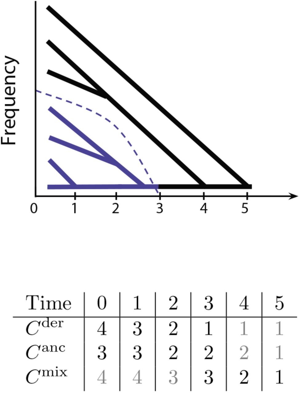
Coalescence conditioned on the allele frequency trajectory (dashed blue line). Blue lineages subtend the derived allele, whereas black lineages do not. Black lineages belong to the ancestral class while the derived allele has Xt > 0, and they belong to the mixed class while Xt = 0. Bottom: the numbers of derived, ancestral, and mixed lineages at each time point. Black numbers factor into the likelihood calculation, whereas gray numbers do not.
We model the probability of transitioning from Ci → Ci+1 lineages during some time interval [ti, ti+1] using a simple variation on Tavare’s formula for the exact distribution of the number of lines of descent remaining after t generations [39] We use Tavare’s formula in order to model the coalescent at discrete timepoints, allowing multiple coalescences at each epoch.
We write the likelihood of a trajectory X given C as

More precisely, in terms of the derived, ancestral, and mixed processes,
 where i*:= max{i: Xi > 0} denotes the index of the epoch during which the allele arose via mutation. Naturally, the mixed process—which we only keep track of while the derived allele is nonexistent—does not depend on X. We can write the transition probabilities using Tavare’s formula [39]:
 where
where

We note that this formula is known to be computationally unstable for large values of C, large values of N, and/or small values of Δti = ti+1 − ti; under such conditions, the asymptotic distribution of Cįi+1 | Ci = a (where a is, e.g., the number of derived lines of descent present at ti) takes on a normal distribution [40]:
 where
where
 and
and
 where α = aΔt/2, β = − Δt/2, and η = αβ/[α(eβ − 1) + βeb] [40]. In practice, for samples of n = 50 haplotypes under constant Ne = 104, we find this approximation is unnecessary; however, for the same sample size under a European demographic model, which exhibits very large recent Ne, we find it necessary to use this approximation during the roughly 103 generations preceding the present day, prior to which Ne, C, and our time discretization (and hence Δt) are sufficiently small that we change over to Tavare’s exact formula [41].
Allele frequency transition probabilities
Our likelihood calculations require allele frequency transition distributions for different selection coefficients, population sizes, and spans of time. Rather than employ the more common approach of numerically calculating allele frequency transition distributions using the Wright-Fisher diffusion process with drift and selection (e.g., [42, 43]), we follow [44] and precompute allele frequency transition distributions on a grid of time spans (i.e., generations) and scaled selection coefficients (i.e., α = 2Ns) using the Wright-Fisher model of reproduction in a finite population experiencing genetic drift and natural selection (see [42]). Specifically, for each value of α, we use simple matrix multiplication to produce allele frequency transition matrices for discrete frequencies in a haploid population of size N = 2000 at a number of generations spanning from g = 1 to g = gmax (corresponding to scaled drift times of 1/2000 to g′ = gmax/2000) with some spacing chosen a priori; in practice, we use linear spacing for recent history and/or periods of population growth. We bin allele frequencies into d discrete frequency categories unevenly distributed between 0 and 1 such that extreme frequency bins outnumber intermediate frequency bins. To calculate allele frequency transition distributions for time spans and selection coefficients not contained in the grid of pre-computed values, we linearly interpolate between the nearest precomputed values. See [44] for details. Additionally, we condition the allele frequency process on the present-day frequency X0 by using the following reweighting:
 where
where  is the forward-time unconditional probability of transitioning from Xi2 to Xi1 (in coalescent time, ti2 > ti1; in forward time, ti2 < ti1). Please see S1 Text for practical documentation on running this procedure.
Marginalizing the hidden allele frequency states
In the previous sections we showed how we obtain  and
and  . The full likelihood of selection given the local tree G is thus

Naively, this involves a prohibitively large sum over dK−1 terms in  , the space of possible trajectories. But due to the conditional independence of the likelihood, we can calculate the likelihood much faster using a recursion:

 and we can apply this recursion to calculate the likelihood function of s given G as

The above is commonly known as the backward algorithm. In our model, the backward algorithm’s recursion proceeds backwards through time. Alternatively, using the forward algorithm, with its recursion proceeding forwards in time:

 and we can apply this recursion to calculate the likelihood function of s given G as

To calculate the posterior probability of the allele frequency during the ith epoch Xi,
 gives the posterior marginal of Xi using the familiar forward-backward algorithm.
Importance sampling to estimate the likelihood function
The above formulas pertain immediately only to the case in which the local tree is observed directly and without noise. In practical settings, the local tree is hidden to us and we must integrate over the space of possible local trees using sampling methods. Here we describe a novel importance sampling method to reweight posterior samples of the ARG to approximate the likelihood function of selection. Although we use s to express the argument of the likelihood function, we use this as shorthand for estimating the likelihood function of arbitrarily complex parameters; for example, one could estimate the selection coefficient s, as well as the time of selection’s onset, ts, before which the allele behaved neutrally.
We are given haplotype data D representing n haplotypes with 1 sites that are fixed for the derived allele. We wish to use D to infer the maximum-likelihood value of s for some locus k ∈ {1, 2,…, l} assuming that all other loci are selectively neutral (i.e. sj = 0 ∀ ∈ {1, 2,…, k − 1, k + 1,…, l}). In other words, we restrict ourselves to testing simple hypotheses of the form “site k has selection coefficient sk and all of its flanking sites are selectively neutral.”
The likelihood of s under the data can be expressed as the expected value of the likelihood of the ARG  given the data D, with respect to the distribution of
  given s:

At this stage, we introduce G, the discrete-time approximation of  (discussed in more detail by [37]), and we assume

By importance sampling, we are able to express the expectation over an alternative distribution q(G), as long as  . Notice that this implies we can conduct sampling under q(G) once, and reweight these samples for arbitrary values of s without having to conduct additional sampling. In other words, approximating L(s) using importance sampling does not require sampling under each value of s at which you want to approximate L(s).
In this paper we specifically consider the estimator given by  ; i.e., the posterior ARG under selective neutrality. Later, we evaluate the performance of the estimator using the Markov chain Monte Carlo method ARGweaver, which samples from the posterior [37]. One can obtain the importance sampling estimate of the full likelihood L(s) by expressing Eq. 16 as an expectation over a different distribution, i.e. the posterior distribution of the ARG (assuming selective neutrality):

We can express Eq. 17 using the Monte Carlo approximation
 where
where  , and “→”, here and in the following, means that the left-hand side converges almost surely to the right-hand side as M goes to infinity, assuming that a Law of Large Numbers for ergodic processes holds (the Birkhoff–Khinchin theorem).
Hence, if we sample genealogies from the posterior under selective neutrality, that is,  , then the right-hand side of Eq. 18 can be used as a Monte Carlo estimator of the likelihood function. However, in practice this estimator is highly unstable. However, a more stable estimator of the likelihood ratio
  can be derived. We can divide through Eq.17 by
  to get

Because we assume the data are conditionally independent of selection given the full ARG, we can simplify this as

A key development in our method is that although we sample the ARG of the entire sequence, we only calculate likelihoods using the marginal tree at the selected site, which we will call Gk. In doing so, we make a key approximation: for differing sweep parameters s and s′, we assume that

That is, we assume that the rest of the ARG is approximately conditionally independent of s given the marginal tree at the selected site, Gk. Thus, we can reduce Eq. 20 to
 which suggests the following importance sampling estimator using genealogies sampled from ARG- weaver will converge almost surely to a close approximation to the likelihood ratio:
 where
where  for m =1, 2,…, M.
Finally, due to exchangeability of lineages within the derived and ancestral allelic classes, we can assume
 where
where
 denotes the summand of the importance sampling estimator. That is, the topology within allelic classes is not important, and instead we need only the lines of descent process within each class.
We can maximize the likelihood ratio over different values of s to obtain the maximum-likelihood estimate of s

Finally, we can obtain an importance sampling estimate of π(xi | D, s), the posterior marginal of the allele frequency at timepoint i, Xi:


Hence,
 where κ is the constant [L(s)/L(s = 0)]−1. Thus, our importance sampling estimate of the posterior marginal given s is
 where in the summand we use the posterior marginal established in Eq. 14. In practice, we fix
  . A concern is, therefore, that this estimator does not take uncertainty in the estimate of s into account. This problem can be addressed by using a Bayesian approach and allowing a prior distribution on s, π(s), the posterior of the selection coefficient π(s | D) follows

Then the estimate of the posterior marginal is given by
 which can be approximated by a sum over d discretized values of s,
  as
as
 where
where  represents a probability mass function over s. In this this paper we assume positive directional selection with a dominance coefficient of h = 1/2, but our method can be extended easily to general values of h as well as negative selection.
The method is implemented in a computer package, CLUES, available for download at https://github.com/35ajstern/clues, with accompanying documentation currently provided in S1 Text.
Simulations
To evaluate the power of CLUES to determine whether a site has been subject to selection, we simulated a dataset of n = 25 diploid individuals under two different demographic models; (1) a model of constant effective population size (N = 104), and (2) a model of European (CEU) demography [45]. We performed both sets of simulations using the program discoal [46]. We set μ = 2r = 2.5 × 10⁻⁸ mut/bp/gen, L =1 × 10⁵ bp or 2 × 10⁵ bp for the constant-size and CEU models, respectively, and simulated conditional on a variety of present-day frequencies and selection coefficients, the latter of which we ranged from weak to strong values. Under each condition, we simulated 100 independent iterations. We also sampled 1 ancient haplotype; because ARGweaver, which we used subsequently to sample the posterior ARG, does not incorporate any information about ancestral/derived states, it is best practice to add an ancient individual or outgroup to help polarize the the alleles. For the constant-size and CEU models, we used ancient sampling dates of 2 × 10⁴ and 1.6 × 10⁴ generations before present, respectively. Because discoal can only simulate piecewise-constant population sizes, we specified population sizes to take on the value of their harmonic mean over the epoch, calculated from the original CEU model. Commands to run simulations of trajectories, local trees, and haplotypes are described in S1 Text.
Importantly, we conditioned simulations on the site of interest segregating at a particular frequency in the present day. Hence, when we considered the power to discriminate between neutral and selected alleles, we controlled the present-day frequency to be equal in both of these cases. Avoiding this step would otherwise upwardly bias estimates of the statistical power, due simply to the tendency for selected alleles to segregate at higher frequencies than neutral alleles [47]. (If the allele frequency in itself is also of interest, this part of the likelihood could trivially be added at a later stage, by simply using the stationary distribution of the allele frequency; see “Allele frequency transition probabilities” under Materials and Methods.) We then simulate the allele frequency backwards in time, from the present-day frequency, until the allele reaches a frequency of 0. Simulators such as discoal achieve this by using the conditional Wright-Fisher diffusion (see e.g. [48]). In the case where effective population size changes over time, running conditional simulations requires additional considerations because the probability of a mutation entering the population scales approximately linearly with population size. Naively sampling the trajectory backwards in time will therefore produce a bias, unless trajectories where the mutation occurs while Ne is low are somehow penalized. Thus, approaches such as reweighting sample trajectories using importance sampling have been used to correct this bias [49]. The program discoal implements a similar bias-correcting scheme using rejection sampling that rejects trajectories where the mutation occurs while Ne is low with higher probability than trajectories where the mutation occurs while Ne is high.
Next, we inferred the posterior ARG given the sequence data we simulated using ARGweaver [37]. This method works by proposing adjustments to an initial ARG, and randomly accepting or rejecting these proposals based on calculations of the prior probability of the proposed ARG, as well as its likelihood given the sequence data. Because the prior probability is based on the effective population size, we specified the same effective population size in the prior as we used to generate the sequence data. We found it important to adjust the proposal mechanism of ARGweaver; specifically, we adjusted resample window size and the number of resamples per window to achieve an acceptance rate of about 30-70%. In total, we sampled 3 × 10³ ARGs for each simulation, discarding the first 1 × 10³ as a burn-in period, and subsequently thinning the remaining samples to reduce the computational burden of downstream analyses; we used a thinning rate of 100 samples, resulting in M = 20 approximately independent samples. Reducing the thinning rate would increase accuracy of the inference at the cost of additional computation to calculate the likelihood of each additional sample tree. Commands to conduct ARG-sampling and local tree extraction are described in S1 Text.
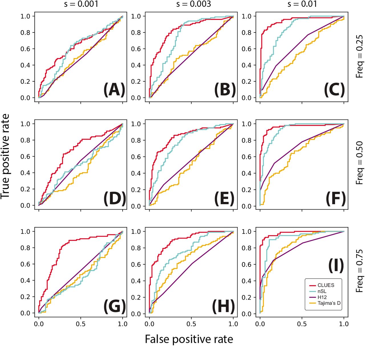
Using utilities in the ARGweaver package, we extracted local trees at the selected site (at the center of the locus) from these sample ARGs. We then analyze this final set of trees using CLUES. We also analyzed the same sequence data using nSL, H12, and Tajima’s D [14, 19, 50]. The nSL method is essentially equivalent to iHS [11], except nSL does not require specifying a genetic map; despite this, these methods have been shown to have very similar statistical power with a slight advantage of nSL under some conditions. H12 is a method to calculate haplotype homozygosity merging the two most common haplogroups; thus, it is a test for selection that is robust to the origin of a sweep, i.e. whether it is hard or soft. Tajima’s D is a site frequency spectrum-based statistic which is sensitive to skews in the frequency distribution of linked alleles caused by hitchhiking on the partially swept selected allele. We used scripts provided by [22] to calculate D and H12, using a window size of 100kb centered on the selected site. We compare testing for selection under these methods by comparing their power curves under both the constant Ne and CEU demography models (Figs. 3,4).

ROC curves illustrating performance of tests between selection and neutrality. Rows correspond to simulations conditioned on the same present-day allele frequency, and columns correspond to simulations with the same value of s. Simulations were performed under a model of constant effective population size (Ne = 104) using a locus of 100kb, n =25 diploid individuals and μ = 2.5 × 10⁻⁸ mut/bp/gen, r = 1.25 × 10⁻⁸ recombinations/bp/gen.
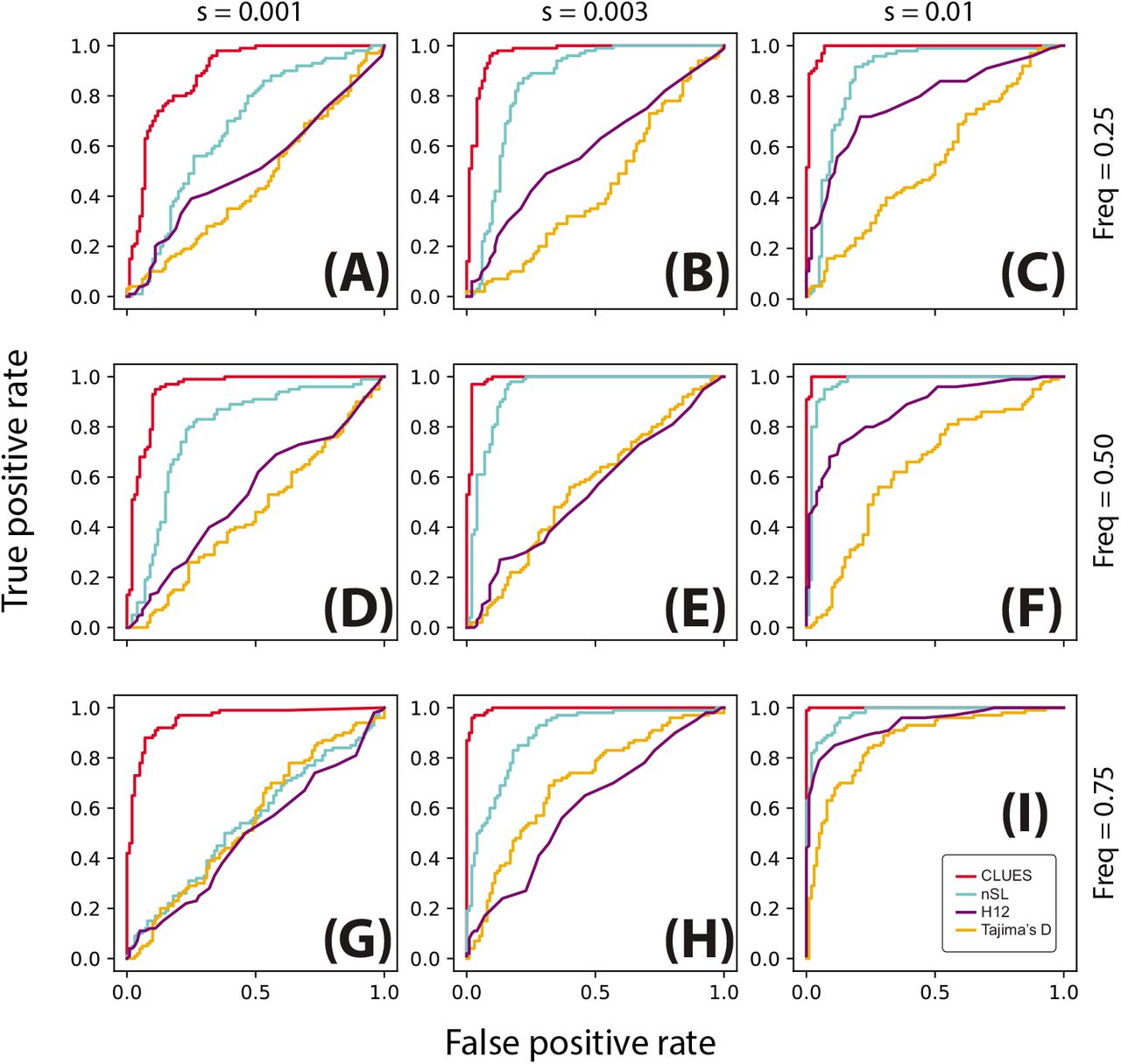
ROC curves illustrating performance of tests between selection and neutrality. Rows correspond to simulations conditioned on the same present-day allele frequency, and columns correspond to simulations with the same value of s. Simulations were performed under a model of European demography using a locus of 200kb, n = 25 diploid individuals and μ = 2.5 × 10⁻⁸ mut/bp/gen, r = 1.25 × 10⁻⁸ recombinations/bp/gen.
We also conducted a similar simulation study for detecting recent selection starting 100 generations ago. We simulated under the same CEU demographic model as previously described, but instead sample n = 50 diploids. We conducted ARG sampling and thinning as previously described, but in our analysis of the sample trees using CLUES, we calculated the likelihood for models of selection where s = 0 up until 100 generations ago, and s ≥ 0 from that point until the present day. This sweep from standing variation (SSV) model differs from the hard sweep model we used previously, which assumes s is constant throughout history. Instead of optimizing the likelihood function just for s, we optimized jointly over two parameters, s and the onset of selection ts, the latter of which represents the time of the onset of selection.
Results
Testing for selection
We found that across all scenarios, CLUES matches or exceeds the statistical power of the other methods evaluated (Figs. 3,4). As expected, all methods had highest power under large values of both the selection coefficient and the derived allele frequency (Fig 3I). Under these conditions, CLUES had 100% power at the 1% significance threshhold; the next most powerful method, nSL, had 68% power at the same significance level. CLUES also demonstrated improvement in power under weak selection; as the selection coefficient was decreased, nSL retained about 20% power when s = 0.003 and <5% power when s = 0.001, and Tajima’s D and H12 retained <5% power under both s = 0.001, 0.003 (Fig 3G,H). By contrast, CLUES retained approximately 45% and 90% power under s = 0.001, 0.003, respectively. We conclude that CLUES has high power across a wide regime of selection strengths, and has notably improved power over standard methods under weaker values of s.
We also considered the effect of present-day allele frequency on statistical power. Previous studies have shown a strong dependence of power on current allele frequency, with methods such as nSl and iHs having highest power at allele frequencies in the 70-90% range (see e.g. [11]). We tested for selection at alleles ranging in present day frequency from 25% to 75%, and while CLUES showed the expected pattern of increasing power with frequency, it also improved on the performance of other methods at lower frequencies. For example, under strong selection (s = 0.01), the power of CLUES changed from 100% to 90% to 85% as the frequency is decreased from 75% to 50% to 25% (Fig. 3C,F,I). By contrast, the power of the next most powerful method, H12, dropped from approximately 65% to 45% to 15% (Fig. 3C,F,I). Under moderate selection (s = 0.003), these effects were even more drastic, with the power of CLUES and nSL (the next most powerful method in this regime) changing from 90% to 60% to 50% and 20% to 5% to <5%, respectively. We conclude that CLUES has high power compared to standard methods across a wide range of allele frequencies, with the most major improvements in performance occurring when the derived allele is at lower frequencies (<50%). We found that using the approximation due to Griffiths (Eq. 4, [40]) decreased power of CLUES by increasing variability of the null distribution of the likelihood ratios. Hence, for testing under nonequilibrium demography we used the exact lines-of-descent probabilities (Eq. 8). By contrast, as we will later show, we found the approximation given by Eq. 4 for t G [0,1000] to improve estimation of allele frequency trajectories under this demographic model.
We also considered the same testing procedure under non-equilibrium demography, simulating under the previously described model of CEU demography (Fig. 3,4). We found in general reduced power to detect selection under this regime relative to the constant population size regime (Fig. 4I, cf. Fig. 3I), consistent with the well-known confounding of expanding population size with selection [10]. Nonetheless, CLUES demonstrated improved power relative to the competing methods across a wide range of selection coefficients (Fig. 4C,F,I), as well as across a wide range of derived allele frequencies (Fig. 4G,H,I).
Estimating selection coefficients
Using the simulations from the previous section to study statistical power in testing for selection, we used our estimate of the likelihood surface for s to estimate the value of the selection coefficient via maximum likelihood (see Eq. 25). We obtained selection coefficient estimates under importance sampling using ARGweaver (Fig. 5), as well as selection coefficient estimates based on the true local tree observed directly (S1 Fig). Generally, the estimates are approximately unbiased. For example, the mean estimates of s = 0,1 × 10⁻³, 3 × 10⁻³, 1 × 10⁻² were approximately  , 9.6 × 10⁻⁴, 3.2 × 10⁻³, 1.3 × 10⁻² when the present day frequency was fixed to 75% (Fig. 5A). Relative to inference when the true tree is observed, we found that the importance sampling estimates had increased variance, reflecting uncertainty in the tree. For example, we saw increased variability in the importance sampling vs. true tree estimates under constant population size (Fig. 5A vs. S1 FigA), as well as under CEU demography (Fig. 5B vs. S1 FigB). This pattern is consistent with the additional uncertainty in s when the local tree is not observed directly. Notably, we found that importance sampling under a model of CEU demography yields estimates with a slight bias towards lower values of s, especially under strong selection (e.g. s = 0.01).

Inference of selection coefficients of varying strength using importance sampling method based on ARGweaver local trees. A: Constant population size. B: Tennessen CEU model. Marker shape denotes the present-day frequency conditioned upon in the simulation: +, 25%; ◯, 50%; ◇, 75%.
Inferring allele frequency trajectories
Using the same simulations and importance sampling estimates we obtained in the previous sections, we decoded the hidden Markov model (HMM) described in the section Materials & Methods. Specifically, we take ŝ, the maximum likelihood estimate of s, and plug it into the posterior marginal (Eq. 14) to obtain a probabilistic estimate of the allele frequency during a particular epoch; we do this independently for each epoch in our discrete-time model. To get a point estimate, we choose to use the posterior marginal mean; i.e., for each epoch, we choose the mean of the posterior marginal distribution. We illustrate the accuracy of these allele frequency trajectory estimates assuming the true local tree is observed and under importance sampling when the true tree is unknown in Fig. 6. We find that estimates of the allele frequency trajectory are generally unbiased for both true trees (Fig. 6 A,B) and importance sampling (Fig. 6 C,D), with increased variance in the trajectory estimates in the importance sampling setting. We also illustrated variability in true vs. inferred trajectories controlling for s (S6 Fig, here setting s = 0).

Allele frequency trajectories inferred from true trees (top row) and ARGweaver local trees (bottom row). Colored trajectories are inferred, black trajectories are the ground truth. Columns correspond to different initial allele frequencies (left: 25%, center: 50%, right: 75%), and rows/colors correspond to different selection coefficients. For each condition we show 25 randomly selected simulations and their corresponding inferences. All data are simulated under a model of constant effective population size (Ne = 104).
Whereas inference tended to be relatively accurate for high-frequency alleles (Fig. 6 B,D), when the derived allele was simulated conditioned on lower frequencies (e.g. 25%, Fig. 6 A,C), estimates tend to be downwardly biased. We tracked this bias to a lack of convergence in ARGweaver; specifically, we found that across different demographic scenarios and selection coefficients, ARGweaver can drastically overestimate the occurrence of very recent coalescences (in our case, in the last 100 generations; see S5 Fig). Under constant population size, we see a nearly 7-fold excess in the number of recent coalescences inferred by ARGweaver. Naturally, this bias will affect estimates for low-frequency alleles more strongly, as fewer lineages subtend the derived allele, and thus a larger proportion of them are susceptible to this bias.
Because recombination rates vary substantially throughout the genomes of humans and other organisms, we also evaluated the accuracy of the estimates assuming μ = r, larger than the μ = 2ρ setting we used in the other simulations, and estimation accuracy to be robust to this increase in recombination rate (S2 Fig).
We also examined trajectory inference under non-equilibrium demography; i.e., the aforementioned model of CEU demography (S3 Fig). Under the CEU model, we found trajectory estimates to have increased variance under importance sampling vs. true trees, but also a slight downward bias in estimating the selection coefficient under strong selection (i.e. s = 0.01; see Fig. 5B, S3 Fig D). As this bias does not occur under the true trees (S1 Fig B, S3 Fig B), we inspected the posterior trees sampled by ARGweaver for patterns consistent with this bias. We found that under this demographic model in particular, ARGweaver tends to under-sample trees with short times to most recent common ancestor (TMRCAs; see S4 Fig). For reference, nearly 60% of runs under constant Ne contained even a single sample tree that had a TMRCA less than or equal to that of the true TMRCA (S4 Fig A). By comparison, under s = 0.01 and CEU demography, only 11% of ARGweaver runs met this criterion (S4 Fig B). Some bias is to be expected, as trees were sampled under a posterior distribution that assumes selective neutrality; however, these results suggest that, if ARGweaver is sampling from the true posterior assuming selective neutrality, then importance sampling estimates (of the selection coefficient, for example) will at least have much higher variance under the CEU model than under constant population size.
We further investigated whether uncertainty in s due to importance sampling variance drove the downward bias when estimating strong selection (Fig. 5B and S3 Fig D). First, we obtained importance sampling estimates of the trajectory fixing s to its true value (S7 Fig A). If uncertainty in s were the cause of the bias, then fixing the true value of s ought to correct for bias due to uncertainty. While we observe less bias in the estimates when fixing the true value of s, the bias is not totally eliminated. We observe a similar reduction in the bias of estimates under neutrality when we fix s = 0 (see S6 Fig B,E,H, vs. S6 Fig C,F,I). Thus, we conclude the bias is due to a lack of convergence in ARGweaver, which appears to be exacerbated in settings where strong selection is combined with non-equilibrium demography.
We also investigated whether incorporating uncertainty in the estimate of s, rather than fixing s = ŝ, would improve the accuracy of trajectory inference. One strategy for modeling uncertainty in s is to apply a prior distribution to s. We found that marginalizing out s with respect to its posterior distribution (assuming a uniform prior on s) did not have a noticeable effect on inference for large values of s (S7 Fig B). This result is concordant with our observation that for large values of s, the likelihood surface peaks so strongly that the posterior remains tightly concentrated around the MLE ŝ. Hence, applying a prior distribution to s does not appear to be an adequate strategy to model uncertainty in s.
Inferring extremely recent selection
We applied our likelihood model of a sweep from a standing variant (SSV) to two types of datasets: selection from a standing variant starting 100 generations ago and selection with constant s (including s = 0), both described in ‘Simulations’ under Materials and Methods. We inferred trajectories under the best case scenario where the true trees are observed (Fig. 7A,B). We found that overall the method inferred the trajectory, as well as the strength and timing of selection, with highest accuracy when selection is strong (e.g. s = 0.03 in Fig. 7A,B). However, we found that as s took on smaller values (s = 0.01), many combinations of s and ts had very similar likelihood (Fig. 7B), and thus estimates of s, ts, and the allele frequency trajectory tended to be noisier than under very strong selection (Figs. 7A,B). Adding the extra parameter ts did not cause overfitting when inferring the trajectories of hard sweeps (Fig. 7A). We also found good power to distinguish between hard vs. soft sweeps (i.e. sweeps from a standing variant), as apparent in the trajectories inferred in Fig. 7A. We calculated statistical power to test for a hard sweep using the statistic  ; intuitively, this statistic is the ratio of the highest likelihood under any model with a SSV (ts ≠ ∞) to the highest likelihood of any hard sweep (ts = ∞). At the 1% significance level we found 60% and 100% power to distinguish soft vs. hard sweeps with s = 0.01, 0.03, respectively.

(A) Trajectories inferred from true trees under both hard sweeps and recent selection on a standing variant (i.e. soft sweeps) when both s and time of selection onset are unknown. (B) The log-likelihood surface for joint inference of s and onset of selection, averaged over 100 simulations, taking the true tree as observed. (C) ROC curves illustrating performance of tests between selection from a standing variant where onset of selection occurs 100 generations ago. We condition on a present day frequency of 50%.
We also performed importance sampling using ARGweaver and evaluated the power of the importance sampling estimates to detect recent selection vs. neutrality (Fig. 7C). Instead of comparing our method to nSL, which is not designed to detect signals of extremely recent selection, we compared to Singleton Density Score (SDS; [21]), as well as H12 and Tajima’s D. We found that for lower values of s, all methods had generally low power. Although CLUES exhibited fairly high power (44%) to detect very strong recent selection (s = 0.03) —even outperforming SDS—we found that H12 has about the same power (45%) in this particular case. The lower power (<5%) of SDS is consistent with the fact that the method was explicitly designed to have high power for large datasets (n > 1000 for selection coefficients of this magnitude). Although we demonstrate that CLUES has substantial power to detect extremely recent selection, we found that importance sampling point estimates of s, ts, and the trajectory were highly vulnerable to biases in the distribution sampled by ARGweaver (S5 Fig). Specifically, we found that across various demographic and selection conditions, ARGweaver samples trees with substantially more recent coalescent events than in the true trees. Specifically, under the European demographic model with the settings used here to study recent selection, we find ARGweaver samples about a 4-fold excess of recent coalescent events (S5 Fig B). Clearly, this bias would produce a false signature of recent selection under neutral conditions. Thus, we did not further explore importance sampling estimates of s and the trajectory under the recent selection model. We conclude that potential ARG-sampling methods that avoid this bias will improve upon power to detect recent selection, as well as point estimates of the strength, timing of selection, and the allele frequency trajectory.
Analysis of a lactase persistence SNP
To assess performance of CLUES on empirical data, we applied our method to study selection acting on the SNP rs4988235 in the MCM6 gene, known to regulate the neighboring LCT gene and affect the lactase persistence trait. The derived allele (A) current segregates at approximately 72% in the 1000 Genomes Phase 3 reference panel (British in England and Scotland, henceforth GBR). We conducted sampling in ARGweaver assuming a model of European demography [45], using a 300kbp region centered around the focal SNP and polarizing alleles using the genomes of three ancient individuals (Altai Neandertal, Denisova, and Vindija Neandertal [51–53]). We sampled M = 200 ARGs, extracted local trees using tools in the ARGweaver package, and conducted importance sampling to estimate likelihood surfaces and trajectories using CLUES.
We found very strong evidence for selection on rs4988235 (s = 0.0161, logLR = 131.82). The trajectory as well as the value of the selection coefficient inferred by CLUES are consistent with previous estimates of the trajectory and s = 0.018 due to Mathieson and Mathieson (2018), illustrated in Fig. 8 [54]. Their method incorporates genomic times series spanning thousands of generations using an HMM-based approach, where hidden states are population-wide allele frequencies, observed states are genotypes of sampled ancient individuals, and transition probabilities are governed by the selection coefficient. Our approach, by contrast, does not utilize any ancient/timecourse data except for the 3 aforementioned ancient individuals, which we use to simply polarize the derived and ancestral states of each allele.

Comparison of inferred allele frequency trajectories for a sweep at rs4988235 (MCM6) in GBR under an ancient DNA (aDNA) based method vs. CLUES, which only uses contemporary modern data. Black curve is the posterior median allele frequency, whereas gray areas are a 95% posterior interval. The red surface is posterior of the frequency trajectory within Steppe ancestry conditioned on an ancient DNA time series, adapted from [54].
Analysis of pigmentation alleles
Using the same GBR panel from 1000 Genomes Phase 3, we analyzed a set of SNPs associated with pigmentation-related traits, some of which were previously identified as likely targets of recent selection [21]. We conducted sampling in ARGweaver assuming a model of European demography, using a 300kbp region centered around the focal SNP and sampling M = 200 approximately iid ARGs. We ran CLUES and estimated likelihood surfaces and allele frequency trajectories for these SNPs (Fig. 9). We found significant concordance between the SDS values and our likelihood ratio statistics paired for each SNP (p = 1.7×10⁻³, Spearman one-sided) [21]. We also illustrated the geographical distribution of these SNPs among diverse populations (S8 Fig) using GGV [55].

Allele frequencies trajectories inferred for 11 pigmentation-associated SNPs in GBR.
We found several signals of very strong selection acting on rs619865 (ASIP, s ≈ 0.10, Fig. 9I), rs12821256 (KITLG, s ≈ 0.016, Fig. 9H), and rs1393350 (TYR, s ≈ 0.011, Fig. 9J); these SNPs are significantly associated with freckling, blonde hair color, and freckling and blue/green eye color, respectively [56–58]. Interestingly, these SNPs all demonstrated a signal of selection mostly concentrated in the last ~5 kya. The geographical distribution of the frequency of these SNPs shows that the derived version of these variants are mostly concentrated in European populations, with minimal sharing with populations located in Africa and Asia (S8 Fig I,H,J). For example, TYR and KITLG segregate at a frequency ~20% in several European populations and have a frequency close to 0% in African and East Asian populations (S8 Fig J). These three SNPs are the only ones in this set of SNPs which have a frequency of nearly 0% across the African populations surveyed, with the exception of OCA2/HERC2 (S8 Fig A,H,I,J), consistent with our evidence for recent selection at these loci. The frequencies of these variants in GBR ranges from ~10-20%; by contrast, the only other variant in this set with comparable frequency in GBR (13%), rs35264875 (TPCN2), we find inconclusive evidence of selection (Fig. 9F), consistent with its comparably even geographical distribution relative to the aforementioned SNPs at ASIP, KITLG, and TYR (S8 Fig F).
At rs12896399 (SLC24A4, Fig. 9B), a SNP identified to be significantly associated with hair color [57], we found strong evidence for moderate selection (s ≈ 0.005). This result is consistent with a previous analysis that suggested positive selection acted on this allele in Out-of-Africa (OoA) populations, based on its high allele differentiation relative to a YRI panel, and low haplotype diversity within CEU individuals [58]. Our results, paired with the apparent low levels of differentiation between European and Asian populations relative to differentiation between OoA populations and African populations at this locus (S8 Fig B) are consistent with our estimate that selection acted on SLC24A4 as early as ~30 kya, during the OoA bottleneck as inferred by [45, 59].
Notably, we find moderate evidence for selection on rs12913832 (OCA2/HERC2, Fig. 9 A, S9 Fig), a SNP previously shown to be causal for blue-brown eye color [60] and significantly associated with hair color [57]. This gene exhibits abberantly high differentiation across populations [61], consistent with a model of local adaptation of eye color. Compared to previous estimates based on ancient DNA samples [62], we estimate substantially weaker selection acting on this gene (s ≈ 0.002 vs. s ≈ 0.04), and we find no evidence to support a recent increase in selection acting on this SNP (i.e., our method found a hard sweep to have higher likelihood than a SSV). Our estimate of moderate selection and lack of a recent change in the selection coefficient imply that selection on OCA2/HERC2 began at least ~50 kya, roughly the time of the start of the OoA bottleneck estimated by [45, 59]. Our analysis suggests that selection on OCA2/HERC2 may have begun much earlier than previously suggested [62].
One surprising result is that we found no signal of selection acting at rs13289810 (TYRP1, s ≈ 0, Fig. 9E). In Europeans, TYRP1 is associated with hair and eye pigmentation [63–66]. Some analyses of European populations have indicated evidence for positive selection on TYRP1 [58, 64, 66]. Our results temper these claims, and appear consistent with the fairly even geographical distribution of rs13289810 frequency across European, African, and Middle Eastern populations (S8 Fig E).
Discussion
We have developed an approach to use modern population genomic data to approximate the full likelihood of selection acting on a locus. We use this approach to test for and estimate the strength and timing of selection, as well as estimate the full allele frequency trajectory. The method is effective across a span of selection coefficients (s = 0 — 0.01), derived allele frequencies (f = 25% –75%), and under multiple demographic models.
Our method draws on previously published methods to estimate the ancestral recombination graph (ARG). We chose to use ARGweaver because it is the only currently available method for sampling the posterior of the ARG; as shown in our derivation of the importance sampling estimates, we rely on sampling from the posterior in order to make rigorous guarantees regarding convergence and consistency of our estimators. Intuitively, it is important to model the uncertainty in the local tree in order to marginalize out this latent variable. We showed that estimates of the selection coefficient and the trajectory are generally accurate, barring scenarios where importance sampling is inefficient, or ARGweaver produces a bias in the inferred trees. In light of these biases, under certain conditions—primarily when the derived allele is at low frequencies (≤ 25%)—importance sampling using ARGweaver trees has limited power to detect selection.
Another important limitation of ARGweaver is its computational cost; in order to study selection on short timescales, large sample sizes are necessary, often on the order of thousands of individuals [21]. The runtime of ARGweaver grows dramatically with increasing sample size; not only does the cost of the individual sampling steps increase with sample size, but also so does the size of the state space, necessitating more samples be taken in order to achieve convergence to the stationary distribution.
However, we see potential to make use of recent advances in inference of local trees in order to further advance approximate full-likelihood methods to infer selection (see e.g., [67–70]; it is worth noting that some of these methods, such as [70], do not infer the ARG in a strict sense, but rather the sequence of local trees along a recombining locus). A major benefit of these methods is that they are far more scalable than ARGweaver, and hence offer more potential to study selection on short, punctuated timescales. However, they also possess several limitations: Firstly, several of these methods only infer topologies, rather than branch lengths [68, 69]. While it is possible to infer branch lengths condition on topology estimates, it is unclear how accurate these estimates would be. By contrast, methods that infer branch lengths along with topology entail a slight tradeoff in their scalability [67, 70]. Another limitation of these methods it that they only yield a point estimate of the local tree, rather than estimating uncertainty in the tree. Nonetheless, it may be feasible to quantify uncertainty in the local tree using a jackknife approach where the local tree is inferred over random subsets of the individuals.
It may also possible to make use of recent advances in inferring pairwise coalescence times (e.g., [71]) to build an approximation to the full likelihood. Recently, Albers & McVean proposed a composite likelihood method to estimate allele age by “sandwiching” the age using identity-by-descent tracts at the site of interest [72]. However, their method does not extend to inferring how the allele frequency changed over time, and does not explicitly model selection.
Currently our method assumes correct knowledge of the demographic history. The effects of latent or mis-specified population structure on inference of selection are well known (e.g., [73]), but in future work one might try to determine the exact effects of mis-specification of effective population size on both inferring the local tree, and inferring selection conditional on the local tree. One approach to dealing with this is to extend the importance sampling approach we use to correct for selection to additionally correct for demography, when ARG sampling is performed under a mis-specified demographic model.
Furthermore, many aspects of our model of selection (e.g. coalescence, allele frequency transitions) assume a panmictic population. To extend our model to more complex demographic models would entail drastically increased computational cost (e.g., marginalizing allele frequencies corresponding to each population, rather than the allele frequency in a single population). Using a deterministic approximation of the allele frequency trajectory would circumvent this issue, but it would also raise new issues, such as how to model allele frequencies when s = 0.
Despite its limitations, the method presented here provides the first close approximation to a full likelihood function for the selection coefficient under simple models. As demonstrated by our simulations, full likelihood methods have the potential to greatly improve power to detect selection and estimate the strength of selection under a variety of conditions. It also provides a rigorous and accurate method for estimating allele frequency trajectories, and is the first to achieve so using modern data. As methods for inferring ARGs improve in the future, so too will the derived methods for detecting and quantifying selection and inferring allele frequency changes.
Funding
RN was supported by (NIH) R01GM116044.
Author contributions
AJS: Conceptualization, formal analysis, investigation, methodology, software, validation, visualization, writing (original draft), writing (review and editing); PRW: Software, writing (original draft); RN: Conceptualization, methodology, supervision, writing (original draft), writing (review and editing).
Potential competing interests
We have no competing interests to report.
Simulations of trajectories, local trees, and haplotypes
To simulate data, we used a slight modification of the standard discoal package [46], available at https://github.com/kern-lab/discoal. In the standard discoal, there is no option to output the allele frequency trajectory, and there is also no option to simultaneously output the sample’s local trees and haplotypes. This is important in order to compare inference vs. ground truth for the same replicate. Our modified version prints the trajectory to stdout, as well as the local trees and the haplotypes, and is available on the CLUES Github page. Nonetheless, the standard discoal documentation applies completely to our modified version, and we will leave the reader to learn the exact meaning of the arguments and options from documentation available through that repository.
To simulate data under the constant effective population size model, we ran
$ ./discoal 51 100 100000 -t 100 -r 50 -A 1 0 0.5 -x 0.5 -c 75e-2 -ws 0 -a 200 -N 10000 -i 4 > example.const.discoalThis specifies a sample of 50 modern haplotypes, simulated independently 100 times, with N = 104 diploid individuals, 4Nμ = 100, 4Nr = 50, and 1 ancient haplotype from 0.5 coalescent units ago. We specify the selected site to be in the center of the locus, segregating at 75% frequency in the present day, with a selection strength of α = 200 = 2Ns where s = 0.01. We simulate the trajectory assuming a time discretization of 1/(4N) coalescent units, on the order of 1 generation.
To simulate data under the European demographic model, we ran $ ./discoal 51 100 100000 -t 3760 -r 1880 -A 1 0 0.021 -x 0.5 -c 75e-2 -ws 0 -i 4 -a 3762 -N 188088 -en 0.000120 0 0.124319 -en 0.000272 0 0.042569 -en 0.000399 0 0.031529 -en 0.000532 0 0.023182 -en 0.000665 0 0.017045 -en 0.000797 0 0.012532 -en 0.000930 0 0.009214 -en 0.001063 0 0.006576 -en 0.001224 0 0.009894 -en 0.001329 0 0.009894 -en 0.001595 0 0.009894 -en 0.001994 0 0.009910 -en 0.002713 0 0.076953 -en 0.003722 0 0.076953 -en 0.004918 0 0.076953 -en 0.006247 0 0.076892 -en 0.007870 0 0.038865 -en 0.008507 0 0.038865 -en 0.009304 0 0.038865 -en 0.010367 0 0.038865 -en 0.011962 0 0.038865 -en 0.014621 0 0.038865 -en 0.018608 0 0.038865 -en 0.023925 0 0.038865 -en 0.033229 0 0.038865 -en 0.046521 0 0.038865 -en 0.066458 0 0.038865 -en 0.132917 0 0.038865 -en 0.398750 0 0.038865 > example.ceu.discoal
This specifies a sample of 50 modern haplotypes, simulated independently 100 times, with N = 188088 diploid individuals, 4Nμ = 3760, 4Nr = 1880, and 1 ancient haplotype from 0.021 coalescent units ago (scaled by the present-day effect population size, N = 188088). We specify the selected site to be in the center of the locus, segregating at 75% frequency in the present day, with a selection strength of α = 3762 = 2Ns where s = 0.01. We simulate the trajectory assuming a time discretization of 1/(4N) coalescent units, on the order of 1 generation. We use the -en option in order to scale effective population size to the harmonic mean of the population size during that time interval. $ ./discoal 101 100 100000 -t 3760 -r 1880 -A 1 0 0.021 -x 0.5 -c 50e-2 -ws 0 -a 3762 -f 0.268 -i 4 -N 188088 -en 0.000120 0 0.124319 -en 0.000272 0 0.042569 -en 0.000399 0 0.031529 -en 0.000532 0 0.023182 -en 0.000665 0 0.017045 -en 0.000797 0 0.012532 - en 0.000930 0 0.009214 -en 0.001063 0 0.006576 -en 0.001224 0 0.009894 -en 0.001329 0 0.009894 -en 0.001595 0 0.009894 -en 0.001994 0 0.009910 -en 0.002713 0 0.076953 - en 0.003722 0 0.076953 -en 0.004918 0 0.076953 -en 0.006247 0 0.076892 -en 0.007870 0 0.038865 -en 0.008507 0 0.038865 -en 0.009304 0 0.038865 -en 0.010367 0 0.038865 - en 0.011962 0 0.038865 -en 0.014621 0 0.038865 -en 0.018608 0 0.038865 -en 0.023925 0 0.038865 -en 0.033229 0 0.038865 -en 0.046521 0 0.038865 -en 0.066458 0 0.038865 - en 0.132917 0 0.038865 -en 0.398750 0 0.038865
This specifies the same demographic model as in the previous simulation, except we increase the sample size to 100 haplotypes (and still 1 ancient haplotype). Additionally, to enforce a SSV, we use -f 0.268 to enforce that the allele evolves under selection from the present day back to the point that it reaches a frequency of 0.268, and neutrally leading up to that point. We must simulate the SSV this way because discoal does not have an option to specify the time of selection’s onset. We obtained the frequencies for the -f option by simulating under selection and finding the average frequency of the allele 100 generations before the present.
Reformatting discoal output
It is necessary to parse the output of discoal to not only prepare the input files for ARGweaver (and CLUES, which just uses ARGweaver-formatted data), but also useful to separate trajectories, local trees, and haplotypes into separate data files. We wrote a Python script to run this process, parseDiscoalOutput.py, which is available on our Github page. The command to run this script is $ python parseDiscoalOutput.py example.discoal <length_of_sequence> <num_sites> < num_haps> <out> where you set the arguments to be the length of the sequence in base-pairs, the number of sites in the discoal simulation (in the two examples above, this would be 105), the total number of haplotypes sampled (n = 51), and a basename for output files. This script will generate 3 files, with extensions .traj, .trees, .sites, that hold the trajectory, the true local tree at the site of interest, and the haplotypes reformatted in ARGweaver format, respectively. These files will be generated and named by the index of each replicate simulated in the file example.discoal. Note that currently this script is hardcoded to assume the SNP of interest is located at the center of the locus.
Performing ARG-sampling using ARGweaver
We use the arg-sample function in the ARGweaver package, available at https://github.com/mjhubisz/argweaver, to sample the posterior ARG [37]. This function requires one major input: the .sites we generated in the previous step. However, it is also necessary to provide the proper demographic model, mutation rate, and recombination rate. Furthermore, you should specify the desired length of the MCMC chain (here M = 3000 samples). You can also compress sequence blocks to greatly speed up the process (here we compress down to 25-bp blocks). By default, ARGweaver thins down to every 10th sample, but this option may be adjusted.
To sample ARGs under a constant population size, we run $ ./arg-sample -s example.const.sites -o example.const --age-file N_10000_agefile.txt -- times-file N_10000_timesfile.txt -N 10000 --overwrite --quiet -m 2.5e-8 -r 1.25e-8 - c 25 -n 3000 --resample-window 40000 --resample-window-iters 8 --infsites
To sample ARGs under the European demographic model, we run $ ./arg-sample -s example.ceu.sites -o example.ceu --times-file tennessen_times_fine.txt --age-file tennessen_age.txt --popsize-file tennessen_popsize_fine.txt --overwrite -m 2.5e-8 -r 1.25e-8 -c 25 --quiet -n 3000 --resample-window 100000 --resample- window-iters 8 --infsites
The files that are specified using --times-file, --age-file, and - -popsize-file correspond to specifying the time discretization (in generations), the age of the ancient haplotype used to polarize alleles (in generations), and the population size trajectory. We supply all of the corresponding files on the CLUES Github page.
We also want to point out several tuning parameters: --resample-window and --resample-window-iters adjust the size of the resampling window and the number of resamples to perform on a particular window. Adjusting these parameters can affect the behavior of the MCMC routine by changing how aggressively changes are proposed to the ARG. Increasing the resample window will decrease the acceptance probability of a given proposal, but increasing the number of iterations will increase that probability that any of these proposals will be accepted. These parameters should be adjusted to yield about a 30-70% acceptance rate (Melissa Hubisz, personal communication).
This procedure will output a series of .smc.gz files.
Extracting local trees from ARGweaver samples
We used the smc2bed-all and arg-summarize programs included in the ARGweaver package to extract local trees at the site of selection. Your ARGweaver output has the form example.<k>.smc.gz, where k = 0,10, 20,…, 3000. To run extraction, $ ./smc2bed-all example; ./arg-summarize -a example.bed.gz -r chr:50000-50000 -l example .log -E > argweaver.example.trees
This saves a list of Newick trees extracted from the site 50000 to argweaver.example.trees.
Preliminaries for CLUES
CLUES depends on a probabilistic model for allele frequency changes. Thus, it is necessary to either download our pre-computed transition probabilities for either the constant N = 104 or European demography models (formatted in HDF5 using the h5py package [74]). We provide an example file example.f_75.hdf5, precomputed conditioned on X(0) = 0.75, but one can alternatively compute transition probabilities from scratch for a custom model. We next describe how to do so.
To compute transition probabilities for a set of selection coefficients s1, s2,…sL from scratch, run the following commands: $ python make_transition_matrices_from_argweaver.py <Nsmall> <s1> example.log trans.s_<s1>.h5 --breaks 0.95 0.025 --debug $ python make_transition_matrices_from_argweaver.py <Nsmall> <s2> example.log trans.s_<s2>.h5 --breaks 0.95 0.025 --debug … $ python make_transition_matrices_from_argweaver.py <Nsmall> <sL> example.log trans.s_<sL>.h5 --breaks 0.95 0.025 --debug $ mkdir example_trans_dir; mv trans.s_*.h5 example_trans_dir
The argument Nsmall denotes the population size of the Wright Fisher model used to calculate the times. It should be no greater than ~ 104, and only around ~ 103 if you want it to run quickly; note that this number can be mucher smaller than the “true” population size, and it is scaled down to simply speed up calculations, and results are rescaled to the “true” size. The example. log file is obtained from the ARGweaver run, and it summarizes the actual demographic model.
After completing this step, it is necessary to aggregate the transition probabilities and condition them on present-day frequencies: $ python conditional_transition_matrices.py example.log example_trans_dir/ --listFreqs 0.25 0.5 0.75 -o trans
This will create a HDF5 file called trans.hdf5. This file contains transition matrices conditioned on the present-day frequency being 0.25, 0.50, and 0.75. It may be wise to use a richer set of frequencies by modifying --listFreqs if you are interested in analyzing real data.
To calculate transition matrices under an SSV model, there is a --ssv option. Warning: this will require substantially longer runtime and storage than the model assuming a hard sweep.
Running CLUES
To run CLUES, the minimal command is $ python \clues.py <treesFile> <conditionalTrans> <sitesFile> <popFreq>
For example, $ python \clues.py example.trees example.f_75.hdf5 example.sites 75e-2 --thin 10 -- burnin 100 --output example.clues
The 4 key inputs here are:
treesFile: local trees sampled and extracted from ARGweaver.
conditionalTrans: transition matrices conditioned on selection coefficient and present-day frequency, formatted in HDF5.
sitesFile: the .sites file used by ARGweaver. (This file is necessary to label the trees by derived/ancestral allele.)
popFreq: the present-day allele frequency you’d like to condition on. If conditionalTrans is conditioned on too sparse a grid of present-day frequencies, CLUES will fail if popFreq is too distant from all of the frequencies.
There are also several options you can deploy. Here we show --thin and --burnin, which we use here to treat the first 100 trees in example.trees as burnin, and thin down to every 10th tree in the file after that point. This corresponds to an overall burnin of 1000 samples and an overall thinning rate of 100 trees, assuming you use the baseline ARGweaver thinning rate of 10 trees. The --output option saves the output of CLUES (e.g. the likelihood surface, importance sampling weights, MLEs, trajectory posterior marginals, and more) to a HDF5 file named example.clues.h5.
There are more options available. To run CLUES under an SSV model, simply use the --ssv option. (Note: running --ssv will require a transition probability file computed using the --ssv option in conditional_transition_matrices.py.) To fix the value of s = s′ (rather than optimize over all potential values of s), use the option --selCoeff s′. To deploy a uniform prior on s, use the option --prior. To specify the position of the site of interest, set --posn <position>, which defaults to 50000.
Acknowledgments
We thank Melissa Hubisz and Andrew Kern for extensive help with the software packages ARGweaver and Discoal, respectively. We also thank Graham Coop, Michael Edge, Yun Song, as well as Vladimir Shchur and other members of the Nielsen Lab, for helpful discussions.
References


