

Abstract
We propose a novel approach based on modern deep artificial neural networks (DNNs) for understanding how the morpho-electrical complexity of neurons shapes their input/output (I/O) properties at the millisecond resolution in response to massive synaptic input. The I/O of integrate and fire point neuron is accurately captured by a DNN with a single unit and one hidden layer. A fully connected DNN with one hidden layer faithfully replicated the I/O relationship of a detailed model of Layer 5 cortical pyramidal cell (L5PC) receiving AMPA and GABAA synapses. However, when adding voltage-gated NMDA-conductances, a temporally-convolutional DNN with seven layers was required. Analysis of the DNN filters provides new insights into dendritic processing shaping the I/O properties of neurons. This work proposes a systematic approach for characterizing the functional “depth” of a biological neurons, suggesting that cortical pyramidal neurons and the networks they form are computationally much more powerful than previously assumed.
Introduction
A single cortical pyramidal neuron is a highly complicated I/O device. It typically receives a barrage of thousands of synaptic inputs over its highly branched dendritic tree. In response, an output in the form of a train of spikes is generated in the axon. The information contained in these spikes is then communicated, via synapses, to thousands of other (post synaptic) neurons. Clearly, understanding the relationship between the neuron’s morphology, physiology and synaptic input, and its spiking output is a central question in neuroscience (Stuart and Spruston 2015; London and Häusser 2005)
One early theoretical idea about the neuron’s I/O function is encompassed by the concept of the perceptron (Rosenblatt and F. 1958), which lies at the heart of some of the most advanced pattern recognition techniques to date (LeCun, Bengio, and Hinton 2015). However, whereas the perceptron might be a reasonable approximation for some simple neuron types, recent studies (Stuart and Sakmann 1994; Stuart et al. 1997; Larkum et al. 2009; Schiller et al. 2000; Magee and Johnston 1995; Spruston et al. 1995) suggest that many central neurons, most notably cortical and hippocampal pyramidal neurons and cerebellar Purkinje cells, significantly differ from the perceptron idealization. The basic function of the perceptron, linear summation and thresholding, oversimplifies the plethora of nonlinear regenerative interactions that take place in the neuron’s dendrites before output spikes are generated in the axon. Such major dendritic nonlinearities include the back propagating (Na+- dependent) action potential (BPAP) from the axon to the dendritic tree (Stuart and Sakmann 1994), the multiple local dendritic NMDA-dependent spikes, each of which is triggered by the activation of a cluster of excitatory synaptic on a single dendritic branch (Polsky, Mel, and Schiller 2004a), and the large and prolong Ca2+ dendritic spike at the apical dendrite, which typically gives rise to a burst of Na+ spike in the soma/axon region (Larkum, Zhu, and Sakmann 1999). Indeed, in recent years it has become evident that single neurons can implement much more complicated functions than does a simple perceptron (or an “integrate and fire” point neuron model). Examples for such complicated computational functions of individual neurons could be found in the pioneering theoretical studies of Rall (Rall 1964) and see also (Shepherd et al. 1985; Mel 1992; Koch and Segev 2014; Koch, Poggio and Torres 1982; London and Häusser 2005; Behabadi and Mel 2013; Häusser and Mel 2003; Polsky, Mel, and Schiller 2004; Poirazi, Brannon, and Mel 2003) and review in (Stuart, Spruston, and Häusser 2007).
Previous studies have identified that synaptic inputs arriving at the same branch may reciprocally contribute to the amplification of each other’s contribution to depolarize the membrane potential (Mel 1992). This mechanism involves the recruitment of the voltage-dependent current through NMDA receptors or Na+/CA2+ voltage gated channels (Mel 1992; Segev and Rall 1998; Magee and Johnston 1995; Spruston et al. 1995), but has a limited spatial range. Under some conditions, the co-activation of several synapses on the same dendritic branch will lead to a local dendritic NMDA spike. Hence, it was suggested that a single dendritic branch acts as a non-linear computation unit and the convergence of these units to a final integration point in the soma is equivalent to a two-layer neural network (Häusser and Mel 2003; Poirazi, Brannon, and Mel 2003; Poirazi, Brannon, and Mel 2003). Indeed, a combination of experimental and theoretical studies demonstrated that such an architecture can better predict the transformation of input firing rate to output firing rate, when considering time windows of 600 milliseconds for the calculation of firing rates, and comparing to an integrate and fire model (Poirazi, Brannon, and Mel 2003). Thus, attributing higher computational power to the individual neuron than previously considered (Mel 1992; Poirazi, Brannon, and Mel 2003; Polsky, Mel, and Schiller 2004). However, while the performance of such a two-layer model at a higher temporal resolution (<600 ms time window) has not been tested, it had been demonstrated through experiment and models that the mechanism of recruitment of the voltage-dependent current through NMDA receptors is highly sensitive to the temporal order of activation of the synapses (Branco, Clark, and Häusser 2011; Branco and Häusser 2011; Rall 1964). Recent modeling studies also emphasized the impact of the location and timing of inhibition on the dendritic Ca2+ spike (Gidon and Segev 2012) as well as on the NMDA-spike (Doron et al. 2017).
As briefly described above, the past decades have seen major advances in our understanding how the low-level neuronal mechanisms (e.g. ion channels, synaptic transmission) interact with each other to support the computation of the neuron. However, these were mostly done for coarse temporal resolution (e.g. average firing rate) due to the incredible combinatorial complexity that is imposed by considering the transformation of thousands of synaptic inputs to spike output at the millisecond precision. Here we propose a novel approach towards this challenge by utilizing recent advances in the field of machine learning, specifically the ability to train deep neural networks to mimic potentially very complex input-output mappings. This allows us to take on the challenge of modeling cortical neurons in its full complexity – considering both excitatory and inhibitory inputs that arrive at arbitrary spatial and temporal patterns to the neuron and attempting to compactly predict its output at the temporal resolution of milliseconds. In addition, we can then use the interpretability characteristics of DNNs to gain additional insights about the function of cortical neurons. This approach enabled us to perform a systematic characterization of the functional “depth” of a single biological neuron and consequently, to demonstrate that cortical pyramidal neurons (and the networks that they form) are potentially much more computationally powerful than previously assumed.
Results
Our goal is to fit the I/O relationship of a neuron by an analogous DNN such that the DNN will receive, as a training set, the identical synaptic input and axonal output of the modeled neuron and, by changing the connection strengths of the DNN using a standard back propagation learning algorithm, the DNN will replicate the I/O transformation of the respective neuron. In order to test the feasibility of such a paradigm and demonstrate its effectiveness, we have started with the I/O transformation of well understood neuron model, that of the integrate and fire (I&F) neuron (Burkitt 2006). What is the simplest DNN that faithfully captures the I/O properties of this most basic single neuron model? To answer this question, we constructed the simplest DNN, consisting of one hidden layer with a single hidden unit (Fig. 1A). The I&F modeled neuron receive a train of random input synapses and produces a subthreshold voltage response and spiking output (see Methods). The analogous DNN received identical input and, after learning, should produce a similar output. To accommodate for the temporal aspect of the input, we chose to employ temporal convolutional networks (TCN) throughout the study. We divided the time axis into 1ms time bins, in which only a single spike can occur. The objective of the DNN network is to predict the binary spike output at time t0 of the I&F model, based on the preceding input spike trains up to that time point. This input is represented using a binary matrix of size Nsyn × T, where Nsyn is the number of input synapses and T is the number of preceding time bins considered (Fig. 1B). We used an I&F neuron model receiving Nsyn = 100 and trained a DNN with a single hidden unit using the back-propagation learning algorithm on 5000 seconds of simulated data. When using T = 80ms we achieved a good fit. Namely, a simple DNN with a single hidden unit accurately predicted both the subthreshold voltage dynamics as well as the spike output at millisecond precision (Fig. 1C).
Figure 1D depicts the weights of the single hidden unit of the respective DNN as a heatmap. It shows that the learning process automatically produced two classes of weights, positive and negative, corresponding to the excitatory and inhibitory inputs bombarding the I&F model. In agreement with our understanding of the I&F model, the excitatory inputs contribute positively to output spike prediction (red color) whereas the inhibitory inputs contribute negatively to output spike prediction (blue color). Earlier inputs, either inhibitory or excitatory, are of less importance to this prediction (teal color). Fig. 1E, depicts the temporal cross-section of those weights (the “filters”) and reveals an exponential profile reflecting the decay of post synaptic potentials in the original I&F model (in reverse time direction). From these filters one can recover the precise membrane time constant of the I&F model. Additionally, there is clear spatial separation between excitation and inhibition. These two temporal filters (excitatory and inhibitory) agrees well with our previous understanding of the temporal behavior of synaptic inputs that give rise to an output spike in the I&F model.
In order to quantify the model performance in terms of spike prediction we use standard binary prediction metrics and compute the Receiver Operating Characteristic (ROC) curve (Fig. 1F left and see Methods) and the area under it. The resulting AUC for the I&F case is 0.997, indicating a very good fit. For an intuitive quantification of spikes temporal precision by the DNN prediction, we plot the cross correlogram between the predicted spike train and the target I&F simulated spike train (the “ground truth”, Fig. 1F right). The cross correlogram shows a sharp peak at 0 millisecond lag, and has a short 10 millisecond half-width, suggesting high temporal accuracy of the DNN. We also quantify the model performance in the task of predicting the subthreshold membrane potential. We use standard regression metrics and plot the scatter plot of the predicted voltage versus the ground truth simulated output voltage (Fig. 1G) and calculate the Root Mean Square Error (RMSE) measure. The resulting RMSE for the I&F case is 1.23mV indicating a very good fit.

(A) Illustration of an I&F neuron model receiving a barrage of synaptic inputs and generating voltage/spiking output (left), and its analogous DNN (right). Orange, blue and magenta represent the input layer, the hidden layer and the DNN output, respectively. (B) Schematic overview of our prediction approach. The objective of the DNN is to predict the spike output of the respective I&F model based on the input spike trains. The binary matrix, denoted by x, represents the input spikes in a time window T (black rectangle) preceding t0. x is multiplied by the synaptic weight matrix, w (represented by the heatmap image) and summed up to produce the activation value of the output unit y. This value is used to predict the output (magenta rectangle) at t = t0. Excitatory input is denoted in red; inhibitory in blue. Note that, unlike the I&F, the DNN has no a priori information about the type of the synaptic inputs (E or I). (C) Top. Example inputs (red – excitatory, blue – inhibitory) presented to the I&F neuron model. Middle. Response of the I&F model (cyan) and of the analogous DNN (magenta). Bottom. Zoom in on the dashed rectangle region in the top trace. Note the great similarity between the two traces. (D) Learned weights of the DNN modeled synapses. Top 80 rows are excitatory synapses to the I&F model; bottom 20 rows are its inhibitory synapses. Columns correspond to different time points relative to t0 (right most time point). One can see that the prediction probability for having a spike at t0 is increased if the number of active excitatory synapses increases (red) and the number of active inhibitory synapses decreases (blue) just before t0. This expected behavior is automatically learned by the DNN. This heatmap represents a spatiotemporal filter of the input. (E) Temporal cross section of the learned weights in D. (F) Left. Receiver Operator Characteristic (ROC) curve of spike prediction; this curve is almost step-like. The area under the curve (AUC) is 0.997, indicating high prediction accuracy at 1ms precision. Inset: zoom in on up to 1% false alarm rates. Red circle denotes the threshold selected for the DNN model shown in C. Right. Cross Correlation between the I&F spike train (ground truth) and the predicted spike train of the respective DNN, when the prediction threshold was set to 0.25% false positive (FP) rate (red circle in left plot). (G) Scatter plot of the predicted DNN subthreshold voltage versus ground truth voltage produced by the I&F model).
In conclusion, as a proof of concept, we have demonstrated that a simple DNN could automatically learn the I/O transformation of a simple I&F model with a high degree of temporal accuracy. The weight matrix (the “filters”) obtained by the learning process exposes known features of the I&F model, such as the differences between excitatory and inhibitory inputs, the temporal summation as a convolution of the synaptic inputs with the exponential decay representing the passive membrane R-C properties and the transformation from subthreshold membrane potential to spike output.
Whereas the I&F model captures many important aspects of real neurons, such as temporal synaptic integration, membrane potential threshold and refractory period, it neglects other known important properties such as spatial integration in dendritic trees, non-linear summation of synaptic inputs and dendritic spikes. Therefore, we next applied our paradigm to a morphologically and electrically complex detailed biophysical model of a 3D reconstructed Layer 5 cortical pyramidal cell (L5PC) from mouse somatosensory cortex (Fig. 2A, left). The model is equipped with a complex nonlinear membrane properties, a somatic spike generation mechanism and an excitable apical nexus capable of generating calcium spikes (Hay et al. 2011; Larkum, Zhu, and Sakmann 1999). At this stage of the model, the excitatory conductance-based synaptic inputs are only of the AMPA-type and of GABAA type for the inhibitory synapses; both are uniformly distributed across the dendritic tree of the model neuron (see Methods). In a similar manner to the previous case for the I&F neuron model, we simulate the cell with diverse randomly generated synaptic activation patterns (see Methods for details) and trained a DNNs on the pairs of input patterns and the resulting output spike trains produced by the model. Fig. 2 shows that we have managed to achieve a good fit when using a fully connected DNN with 128 hidden units and a single hidden layer (Fig. 2A, right). In our experiments, we have failed to achieve a good fit when using the architecture that was previously successful for I&F model neuron in Fig. 1A.

(A) A model of 3D reconstructed L5 pyramidal neuron (L5PC) from the mouse somatosensory cortex (left). Basal oblique and apical dendrites are marked by respective green, purple and orange colors. The analogous DNN for this neuron is shown at right. Orange, blue and magenta circles represent the input layer, the hidden layer and the DNN output, respectively. Green units represent linear activation units (see Methods). (B) Top. Response of the L5PC model (cyan) and of the analogous DNN (magenta) to random AMPA-based excitatory and GABAA-based inhibitory synaptic input (see Methods). Bottom. Zoom in on the dashed rectangle region in the top trace. Note the great similarity between the two traces. (C) Learned weights of a selected units in the DNN, separated by their morphological (basal, oblique and apical) location. In each case, the top half rows are excitatory synapses and the bottom half are the inhibitory synapses. As in Fig 1D, different columns correspond to different time points relative to t0 (right most time point). Note that the output of this hidden unit increases if the number of active excitatory synapses increases at the basal and oblique dendrites (red) whereas the number of active inhibitory synapses decreases (blue) at these locations, just before t0. However, this unit is non-selective to activity at the apical tuft, indicating the lack of influence of the tuft synapses on the neuron’s output. (D) Temporal cross section of the learned weights in C. Note the asymmetry between the temporal profiles of excitatory and inhibitory synapses due to the different synaptic dynamics of AMPA and GABAA synapses. (E) Quantitative evaluation of the fit (as in Fig 1F). Left. ROC curve of spike prediction; the area under the curve (AUC) is 0.961, indicating high prediction accuracy at 1ms precision. Inset: zoom-in on up to 10% false alarm rates. Red circle denotes the threshold selected for the DNN model shown in B. True positive rate (TP) at false positive rate (FP) of 0.25% is 35.8% indicating a relatively high hit rate even for a very low false alarm rate. Right. Cross Correlation plot between the ground truth (L5PC model response) and the predicted spike train of the respective DNN, for prediction threshold of 0.25% FP rate (red circle in left plot). (F) Scatter plot of the predicted DNN subthreshold voltage versus ground truth voltage.
Fig. 2B shows an exemplar test trace for the DNN illustrated in Fig. 2A whereas Fig. 2C shows a representative exemplar of the weight matrix for one of the hidden units of the DNN. This matrix is split into three blocks according to the location of the input synapse on the dendritic tree. By examining the filters of the hidden layer of the DNN we observed that the weights representing inputs to the oblique and basal dendrites had profiles that resembles PSPs (mirrored in time); the basal inputs were on average slightly more efficacious than that on the oblique (Fig. 2C and Fig. 2D). Interestingly, the weights to the apical tuft were essentially zero (Fig. 2C and Fig. 2D, right). This pattern remains consistent for all first layer filters of the network, implying that in this model the apical dendritic synapses had negligible information regarding predictions of the output spikes of the neuron, even in the presence of calcium spikes occasionally occurring in the nexus.
Fig. 2E and Fig. 2F show the quantitative performance evaluation. For binary spike prediction (Fig. 2E), the AUC is 0.961. True Positive rate (TP) at 0.25% False Positive rate (FP) is 35.8%. For somatic voltage prediction (Fig. 2F), the RMSE is 0.85mV and 90.1% of the variance is explained by this model. We note that the due to the relatively low firing rate of the neuron, the binary classification problem of instantaneous spike prediction problem is highly unbalanced. For every second of simulation there are on average 1 positive samples (spikes) for every 999 negative samples (non-spikes). Therefore, we use a very conservative threshold over the binary spike probability prediction output of the DNN in order to create the final spike train prediction and examine the cross-correlation plot. Note that a prediction without a single True Positive can on the 1ms time binning binary spike prediction problem can still be in fact a very good solution, e.g. if our model outputs as its prediction the exact same spike train as the original but offset by 1ms in time. In this case, there will be no True positives, and many False positives, but the predicted spike train is in essence quite good. Namely, the temporal cross correlation between the original and predicted spike trains is not directly related to binary prediction metrics used. We choose 0.25% False positive rates throughout the study since it provides a good trade-off point between true positive and false positive in our case.
Detailed studies of synaptic integration in dendrites of cortical pyramidal neurons suggested the primary role of the voltage-dependent current through synaptic NMDA receptrors, including at the subthreshold and suprathreshold (the NMDA-spike) regimes (Polsky, Mel, and Schiller 2004; Branco, Clark, and Häusser 2010). As NMDA receptors depend nonlinearly on voltage it is highly sensitive not only to the activity of the synapse in which the receptors are located but also to the activity of (and the voltage generated by) neighboring synapses and to their dendritic location. Moreover, the NMDA-current has slow dynamics, promoting integration over a time window of tens of milliseconds (Major, Larkum, and Schiller 2013, Doron et al., 2017). Consequently, we hypothesized that adding NMDA dependent synaptic current to our L5 PC model will significantly increase the depth of the respective DNN.
As an illustrative example, we first attempted to fit the somatic voltage of a Layer 2/3 Pyramidal Cell (L23PC) taken from the visual cortex of the mouse (Branco, Clark, and Häusser 2010) in response to random activation of only 9 excitatory synapses uniformly distributed across a single dendritic branch (Fig. 3A). We found that a single dendritic branch with NMDA synapses is faithfully captured by a single layer of a fully connected DNN with 4 hidden units (Fig. 3A&B). Examining the 4 filters of the first layer reveals interesting shapes that make an intuitive sense (as first explored by the pioneering theoretical studies of (Goldstein and Rall 1974; Rall 1969; Rall 1964). The topmost filter in Fig. 3D appears to be summing only very recent and proximal dendritic activation. The second-from-top hidden unit appears to be summing recent distal dendritic activation. The third filter clearly shows a direction selective hidden unit, preferring distal to proximal synaptic activation patterns, and the last hidden unit appears to be a prolonged distal dendrites summation of activity combined with precisely times proximal input activation.

(A) Left. Layer 2/3 pyramidal neuron used in the simulations with a zoom on one selected basal branch (dashed rectangle). Same modeled branch with 9 excitatory synapses (depicted schematically by the “ball and stick” at bottom) was also used in the study of Branco et al. (Branco, Clark, and Häusser 2010). Right. Illustration of the analogous DNN. Colors as in Fig. 2A. (B) Example of the somatic voltage response (cyan) and DNN predicted output (magenta) to a randomly generated input spike pattern on that basal branch (red dots above). (C) Example of somatic response to two spatio-temporal sequences of synaptic activation patterns (red - distal-to-proximal direction” and blue - “proximal-to-distal direction”) and the DNN predicted output for these same sequences (orange and light blue traces, respectively). (D) Learned weights of the 4 hidden units by the respective DNN model. Heatmaps are spatio-temporal filters as shown in Figs. 1D and 2C. Note the direction selective shapes and long temporal extent of influence by distal synaptic activations. (E) Scatter plot that show the discrimination ability between different order of synaptic activations on the modeled basal branch. Vertical axis is the ground truth maximum voltage at the soma during a specific synaptic order of activation. Horizontal axis is directionality index proposed in Branco et al. (Branco, Clark, and Häusser 2010). Correlation coefficient is 0.86. (F) Same as E, but the DNN’s estimation of the max voltage of the respective order of activation, showing a superior performance of the DNN prediction relative to the directionality index previously proposed. Correlation coefficient is 0.99.
Fig. 3C specifically examines the special cases studied in Branco et al. (Branco, Clark, and Häusser 2010), of sequential activation of the 9 synapses in the distal to proximal direction and, conversely, in the proximal to distal direction. Our DNN network trained on random synaptic activation patterns, successfully replicated this behavior. Fig. 3E shows our reconstruction of the results of Branco et al. (Branco, Clark, and Häusser 2010), whereby a directionality index was suggested as a possible predictor for the peak somatic voltage for random activation sequence of the 9 input synapses. Fig. 3F shows the prediction of the respective DNN for the same sequences as in Fig. 3E. Interestingly, our DNN acts as a much better predictor for the peak somatic voltage. It is important to note that the special case of 9 synaptic activations equally spaced in time is highly unlikely to occur during the random input stimulation regime which was used to train the DNN. Nevertheless, the network can generalize even to this new input regime with high precision.
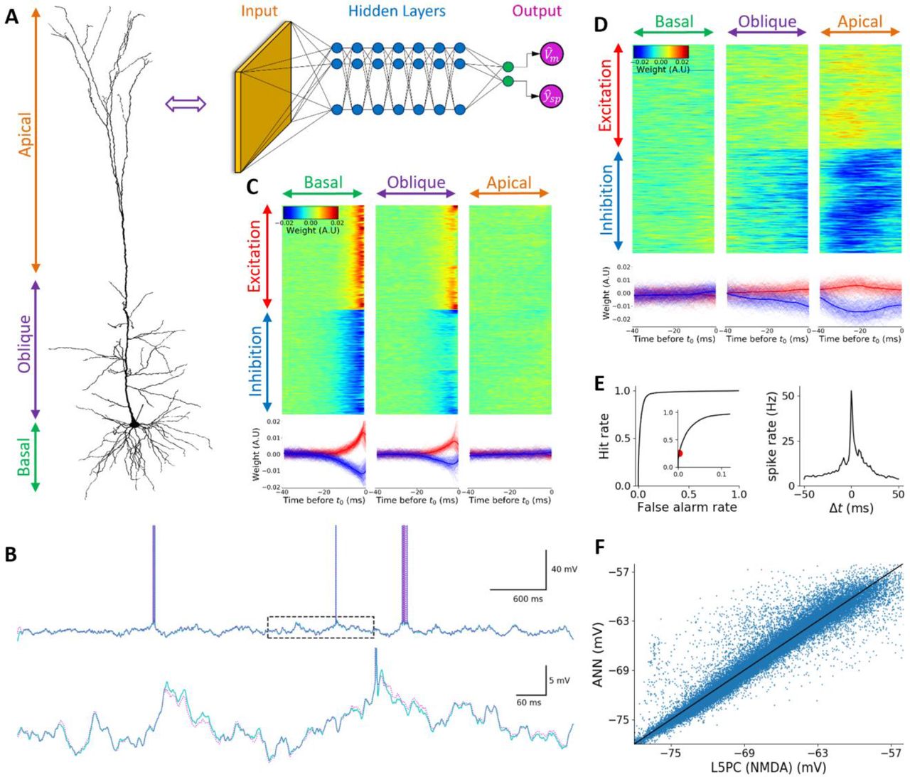
Fitting a single dendritic branch with NMDA based synapses confirmed our initial expectation of the complexity they add to the I/O transformation. Therefore, our ultimate challenge was to fit a realistic L5PC model (such as the one used in Fig. 2) but with the addition of NMDA-based synaptic conductance added to the excitatory synapses (on top of the AMPA-conductance). A thorough search of configurations of deep and wide fully connected neural networks have failed to provide a good fit. These failures suggest a substantial increase in the complexity of I/O transformation. We found that only a deep temporally convolutional network (TCN), with 7 layers and 128 channels per layer provided a good fit. The accuracy of the model was insensitive to the temporal kernel sizes of the different DNN layers when keeping the total temporal extent of the entire network fixed, so the temporal extent of the first layer was selected to be larger than subsequent layers mainly for visualization purposes.
Fig. 4C shows a filter from a unit at the first layer of the DNN. This filter is similar to the filter in Fig. 2C in the AMPA-only case. Fig. 4D, however, shows a filter of another unit, which in contrast to the model in Fig 2, has negligible weights assigned for basal and oblique dendrites but a very strong apical tuft dependency. This filter hints to the fact that the NMDA non-linearity greatly assists in the activation of apical tuft dendrites. By examining additional first layer filters we can see a wide variety of different activation patterns that the TCN utilized as intermediate representation, including temporally directionally selective filters (similar to those of Fig. 3D). Fig. 4E and Fig. 4F show the quantitative performance evaluation. For binary spike prediction (Fig. 4E), the AUC is 0.969. True Positive rate (TP) at 0.25% False Positive rate (FP) is 25.2%. For somatic voltage prediction (Fig. 4F), the RMSE is 1.13mV and 91.4% of the variance is explained by this model. It is important to note, that despite its seemingly large size the resulting DNN is shows substantial computational improvement relative to the detailed biophysical model as indicated by the 2000-fold speedup of simulation time.

(A) Illustration of L5PC model (left) and its analogous DNN (right). As in previous figures, orange, blue and magenta circles represent the input layer, the hidden layer and the DNN output, respectively. Green units represent linear activation units (B) Top. Exemplar voltage response of the L5PC model with NMDA synapses (cyan) and of the analogous DNN (magenta) to random synaptic input stimulation. Bottom. Zoom in on the dashed rectangle region in the top trace. (C) Learned weights of a selected unit in the first layer of the DNN. Top Left, top center and top right, inputs located on the basal dendrites, on the oblique dendrites and on the apical tuft, respectively. For each case, top half of the rows are excitatory synapses whereas bottom half of rows are its inhibitory synapses. Different columns correspond to different time points relative to t0 (right most time point). Bottom. temporal cross-section of the learned weights above. Note the great similarity of this unit to the unit shown in Fig. 2C. (D) Similar to C, for a different unit in the first layer but with a completely different spatio-temporal pattern. This unit appears to be non-selective to whatever happens in the basal dendrites, only slightly sensitive to oblique dendrites, but very sensitive to apical tuft dendrites. The output of this hidden unit is increased when there is apical excitation and lack of apical inhibition in a time window of 40ms before t0. Note the contrast to the DNN model of L5PC with only AMPA synapses that practically ignored apical tuft dendrites. Additionally, note the asymmetry between the amplitudes of the temporal profiles of excitatory and inhibitory synapses, indicating that inhibition decreases the activity of this unit more than excitation increases its activity. (E) Quantitative evaluation of the fit. Left. ROC curve of spike prediction; the area under the curve (AUC) is 0.969, indicating high prediction accuracy at 1ms precision. Zoom in on up to 10% false alarm rates is shown in the inset. Red circle denotes the threshold selected for the DNN model shown in B. True positive rate (TP) at false positive rate (FP) of 0.25% is 25.2%, indicating a relatively high hit rate even for a very low false alarm rate. Right. Cross Correlation plot between the ground truth (L5PC with NMDA synapses) spike train and the predicted spike train of the respective DNN, when the prediction threshold was set to 0.25% false positive rate (FP) (red circle in left plot). (F) Scatter plot of the predicted DNN subthreshold voltage versus ground truth voltage.
Discussion
Neurons are the computational building blocks of the brain and, therefore, understanding their input-output (I/O) transformation has been a fundamental question in neuroscience since “the neuron doctrine” by Ramon Y Calal. Early theories (McCulloch and Pitts 1943; Lapicque 1907) have captured some essential properties of this I/O process, such as the temporal integration of synaptic inputs and the threshold non-linearity associated with action potential generation. Later theories (Rall 1964; Rall 1967) have accounted for phenomenon discovered in experiments such as effects of dendritic location of synaptic signals and interaction between excitation and inhibition. Over the past few decades, experimental studies have exposed many spatially-distributed nonlinear membrane and synaptic mechanisms in dendrites that equip single neurons with the capability to perform very complex I/O transformation (London and Häusser 2005; Stuart and Spruston 2015). Thanks to the introduction of compartmental models (Rall 1964) and digital anatomical reconstructions, we can now account for nearly all those experimental phenomena, as well as explore conditions that are not accessible with current experimental technique. In that sense we have developed along the last 50 or so years a faithful model of the input-output transformation of neurons. Unfortunately, this comes at a price. Simulation of compartmental models entails numerically solving thousands of coupled nonlinear differential equations which is computationally intensive (Segev and Rall 1998; Burke 2000). Moreover, while the simulation provides good fit to data, it is not optimized for providing conceptual understanding of the process by which it is achieved.
Simple conceptual models to address this problem were previously suggested by B. Mel and colleagues (Poirazi, Brannon, and Mel 2003; Poirazi, Brannon, and Mel 2003; Polsky, Mel, and Schiller 2004), and though they achieved their goal of providing a conceptually easy framework for understanding I/O properties of neurons, they failed to account for the full complexity of neuron’s functioning as they have only considered the spatial integration properties at temporal resolution of seconds (namely, only rate coding). In this work we demonstrate a much-improved model in terms of fitting accuracy, while remaining conceptually simple and, indeed, providing new insights into how the neuron’s morphology, membrane nonlinearity and spatio-temporal synaptic properties shape the I/O relationship of neurons. Recent advances in the field of deep neural networks, provide, for the first time, a powerful general-purpose tool that can learn a mapping of I/O relationships from examples, including that of single complex nonlinear neurons, as demonstrated by this work. We have chosen to apply this framework to a series of neuron models with increasing levels of morpho-electrical complexities. We constructed a large dataset of pairs of input-output examples by simulating a neuron receiving rich repertoire of synaptic inputs and recorded its output in terms of spikes at millisecond precision as well as its subthreshold membrane potential. We then trained networks of various configurations on these input output pairs until we obtained an analogous “deep” network with a performance acceptable in the field of machine learning for solving real world problems.
We showed (Figure 1) that for simple neuronal I&F neuron models the framework provides simple DNNs that capture the full I/O relationship and provides key insights that are consistent with our understanding of the I&F models. Surprisingly, Figure 2 shows that even a neuron model, that of layer 5 cortical pyramidal neuron with complex dendritic trees and with a host of dendritic voltage dependent currents is well-captured by a relatively simple network with a single hidden layer. However, the introduction of NMDA currents significantly increases the complexity of the required network. In the case of a single dendritic branch with NMDA synapses, the respective DNN network requires several units to capture different aspect of spatio-temporal integration of synaptic inputs (Figure 3). In a full model of a L5 pyramidal neuron with NMDA-based synapses, the complexity of the network is significantly increased, and we could not fit the data with a temporal-convolutional network that has less than 7 hidden layers (Figure 4).
These results suggest that the single cortical neuron with its nonlinear synaptic inputs is already, on its own, a sophisticated computational unit and that, consequently, cortical networks are “deeper” and computationally more powerful than they seem to be just based on their anatomical connections. Importantly, the implementation of the I/O function using a DNN provides also practical advantages as it is much more efficient than the traditional compartmental model. In our tests we obtained a factor of ~2000 speed up when using the DNN instead of its compartmental-model counterpart. This could have an important contribution for simulating large scale realistic neuronal networks (Markram et al. 2015; Egger et al. 2014)
In addition, the depth of the respective DNN for a given neuron could be used as an index for its computational power; the deeper it is the more sophisticated computations this neuron could perform. Such index will enable a systematic comparison between different neuron types (e.g., CA1 pyramidal cell, cortical pyramidal cell and Purkinje cell, or for the same type of cell in different species e.g., mouse vs. human cortical pyramidal cells).
The analysis of deep neural network is a challenging task and a rapid growing field(Olah, Mordvintsev, and Schubert 2017; Mordvintsev, Olah, and Tyka 2015; Mahendran and Vedaldi 2015). Nevertheless, observing the weight matrix of units (“filters”) in first layer of the respective DNN is fairly straight forward and can provide ample insights regarding the I/O transformation of the neuron. The full network can be interpreted as consisting of a basis set of filters that span the space of possible spatio-temporal patterns of synaptic inputs that will drive the original neuron to spike. The first layer defines this space, and the rest of the network mixes and matches within that space. For example, as shown in Figure 2, in the case of pyramidal neuron without NMDA synapses, most filters have significant weights only for basal and oblique inputs and the weight given for apical tuft synapses is negligible (despite the existence of voltage dependent Ca2+ and other nonlinear currents in this model including occasional Ca2+ spikes). The picture is fundamentally different when NMDA synapses are included in the model. In that case the weight assigned to apical dendrite synapses is significant. Moreover, it is interesting to note that the filters devoted to those inputs tend to have a temporal structure that is significantly wider than proximal synapses, suggesting that the temporal precision of inputs to the apical synapses is less important. These are simple insights that can be drawn by just observing first layer filters of the resulting network.
This work opens multiple interesting investigation avenues for future research. One important avenue is the isolation of the contribution for specific mechanisms to the computational power of the neuron in a similar way done here for NMDA. By fitting a DNN while manipulating specific dendritic currents (e.g. VGCa, Kv, HCN channels) we will better understand their contribution to the overall synaptic integration process and to the “depth” of the respective DNN. An additional avenue of investigation is to utilize this work to improve our understanding of synaptic integration in the dendrites. Rather than modelling a neuron bombarded with random meaningless input, we can utilize our neuron-equivalent-DNN to make the single neuron perform some interesting meaningful function. For example, now that we estimate that a pyramidal neuron is equivalent to a deep network with 7 hidden layers, we can use this DNN to teach the neuron to implement a function which is in the scope of capabilities of such a network, such as classifying hand written digits or a sequence of auditory sounds. We can then both validate our hypothesis, that single neurons can perform complex computational tasks, and analyze how these neurons can implement complex tasks.
Methods
I&F simulation
For Fig.1 simulations, membrane voltage was modeled using a leaky I&F simulation 
 , where wi denotes synaptic efficacy for each synapse, ti denotes presynaptic spike times and K(t − ti) denotes the temporal kernel of each postsynaptic potential (PSP). We used temporal kernel with exponential decay
  where u(t) is the Heaviside function
  and τ = 20ms is the membrane time constant. When threshold was reached, and output spike was recorded, and the voltage was reset to Vrest = −95mv. As input to the simulated I&F neuron Nexc = 80 excitatory synapses and Ninh = 20 inhibitory synapses were used. Synaptic efficacies of wexc = 5mv were used for excitatory synapses and winh = −5mv for inhibitory synapses. Each presynaptic spike train was taken from a Poisson process with a constant instantaneous firing rate. Values used fexc = 3.3Hz for excitatory synapses and finh = 3.2Hz for inhibitory synapses. Resulting output average firing rate for these simulation values was 2.1Hz..
L5PC simulation
For Fig. 2 and Fig. 4 simulations, we used a detailed compartmental biophysical model of cortical L5PC as is, modeled by Hay et. al, 2011. For full description the model please see methods in original paper. Briefly, this model contains in total 12 ion channels for each dendritic compartment. Some of the channels are unevenly distributed throw-out the dendritic arbor. In Fig. 2, double exponential conductance based AMPA synapses were used in simulations with τrise = 0.3ms, τdepress = 3ms and gmax = 0.4nS. For Fig. 4 related simulations we used the standard NMDA model by Jahr and Stevens, 1993, with τrise = 2ms, τdepress = 70ms and gmax = 0.4nS. For both Fig. 2 and Fig. 4, we also use double exponential GABA A synapses with τrise = 2ms, τdepress = 8ms and gmax = 1nS. on each independent dendritic segment, we place a single AMPA (for Fig. 2) or AMPA+NMDA (for Fig. 4) synapse as well as a single GABA A synapse. In order to mimic uniform coverage of excitatory and inhibitory synapses on the entire dendritic tree, we stimulate each compartment with firing rate proportional to the segment’s length. Each presynaptic spike train was taken from a Poisson process with a smoothed piecewise constant instantaneous firing rate. The gaussian smoothing sigma, as well as the time window of constant rate before smoothing were independently resampled for each 6 second simulation from the range 10ms to 1000ms. This was chosen as opposed to constant firing rate to create additional temporal variety in the data in order to increase the applicability of the results to all possible situations. For Fig. 4 simulations with NMDA synapses, total amount of excitatory and inhibitory presynaptic spikes per 100ms ranges between 0 and 800 spikes, which is equivalent to 8000 excitatory synapses with average rates of 1Hz and 2000 inhibitory synapses with average rates of 4Hz. The average output firing rate of the simulated cell across all simulations was 1.5Hz. For Fig. 2 simulations, with AMPA only synapses, total amount of excitatory and inhibitory presynaptic spikes per 100ms ranges were increased twofold in order to account for the smaller amount of total current injected in order to achieve similar output firing rates of 1.5Hz.
L23PC simulation
For Fig. 3 simulations, we used a detailed compartmental biophysical model of cortical L23PC as is, modeled by Branco et. al, 2010. In these experiments we stimulate a single branch with 9 dendritic segments with an NMDA synapse on each compartment, with parameters as in the simulation for Fig. 4. The branch was selected as in Branco et al, 2010 in order to perform comparison with original paper. Similarly, to Fig. 2. And Fig. 4 simulations, each presynaptic spike train was taken from a Poisson process with a smoothed piecewise constant instantaneous firing rate. The number of presynaptic input spikes to the branch per 100ms ranged between 0 and 15 in simulations used for training. In Fig. 3 C,E,F, we repeated input stimulation protocol suggested by Branco et. al, 2010, consisting of single presynaptic spike per synapse with constant time intervals of 5ms between subsequent synaptic activations, only randomly permuting the order of activation between trials.
DNN fitting
In order to represent the input in a suitable manner for fitting by a DNN, we discretize time using 1ms time bin Δt. Using this discretization, we can represent a spike train as a sequence of binary values S[t], such that S[t] ∈ {0,1}, since the length of a spike is approximately 1ms there cannot be more than a single spike in such a time interval. We denote the spike trains the neuron receives as input as X[S, t], S ∈ {1,2, …, Nsyn}, t ∈ {1,2, …, T}, where s denotes the synapse index, and t denotes time. The spike trains a neuron emits as output we denote as yspike[t], The somatic voltage trance we denote as yvoltage[t]. For every point in time, we attempt to predict both somatic spiking yspike[t] and somatic voltage yvoltage[t] based only a Tinput sized window of presynaptic input spikes. i.e. define the vector 
 and a neural network that maps
  to
to  and
and  . i.e.
  . We treat spike prediction as a binary classification task and use standard log loss and treat voltage prediction as regression task and use standard MSE loss. We wish to find a model’s parameters θ such that we minimize a combined loss
  , where wvoltage is the relative importance of the spike prediction loss with respect to the somatic voltage prediction loss. For most of our experiments we set wvoltage to be about half the size of the spike loss. The DNN architecture we use is a temporally convolutional network (TCN) and we apply it in a fully convolutional manner on all possible timepoints. Note that if the temporal filter size after the first layer is 1 in a TCN applied as described, this is effectively a fully connected neural network. In most of our experiments we use fully connected neural networks, except for Fig. 4 in which we used a proper TCN with hierarchical convolutional structure. After every convolutional layer, a batch normalization layer immediately follows. We employ learning schedule regime in which we lower the learning rate and increase batch size as we progress through training. Full details of learning schedule in each case are in the attached code repository.
Model evaluation
We divided our simulations to train, validation and test datasets. We fitted all DNN models on train dataset, all reported results are on an unseen test dataset. Validation dataset was used for modeling decisions and hyper parameter tuning. We evaluate binary spike prediction results using receiver operator characteristic (ROC) curve and calculate the area under curve (AUC). For creating a binary prediction, we choose a threshold that corresponds to 0.2% false positive rate. In order to evaluate the temporal precision of the binary spike prediction we plot the cross-correlation between the predicted output spike train and the ground truth simulated spike train. In order to evaluate the voltage prediction, we calculate the RMSE and plot the scatter plot between predicted voltage and the ground truth simulated voltage.
Code and data availability
All data and code used for this work will soon be published.
Acknowledgements
We thank Oren Amsalem, Guy Eyal, Michael Doron, Toviah Moldwin and all lab members of the Segev and London Labs for many fruitful discussions and valuable feedback regarding this work. This work was supported by a grant from the EU Horizon 2020 program (720270, Human Brain Project), a grant from the Gatsby Charitable Foundation and by Huawei Technologies Co. Ltd.


