Fast and Accurate Clustering of Single Cell Epigenomes Reveals Cis-Regulatory Elements in Rare Cell Types

Abstract

Mammalian tissues are composed of highly specialized cell types defined by distinct gene expression patterns. Identification of cis-regulatory elements responsible for cell-type specific gene expression is essential for understanding the origin of the cellular diversity. Conventional assays to map cis-elements via open chromatin analysis of primary tissues fail to resolve their cell type specificity and lack the sensitivity to identify cis-elements in rare cell types. Single nucleus analysis of transposase-accessible chromatin (ATAC-seq) can overcome this limitation, but current analysis methods begin with pre-defined genomic regions of accessibility and are therefore biased toward the dominant population of a tissue. Here we report a method, Single Nucleus Analysis Pipeline for ATAC-seq (SnapATAC), that can efficiently dissect cellular heterogeneity in an unbiased manner using single nucleus ATAC-seq datasets and identify candidate regulatory sequences in constituent cell types. We demonstrate that SnapATAC outperforms existing methods in both accuracy and scalability. We further analyze 64,795 single cell chromatin profiles from the secondary motor cortex of mouse brain, creating a chromatin landscape atlas with unprecedent resolution, including over 300,000 candidate cis-regulatory elements in nearly 50 distinct cell populations. These results demonstrate a systematic approach for comprehensive analysis of cis-regulatory sequences in the mammalian genomes.

Introduction

Mammalian tissues comprise of various cell types highly specialized to carry out distinct functions. Cellular identity and function are established and maintained through programs of gene expression that are specific to each cell type and state¹. Gene regulation is carried out by sequence-specific transcription factors that interact with cis-regulatory sequences, such as promoters, enhancers and insulators². Identifying cis-regulatory elements in the genome is an essential step towards understanding the cell type specific gene regulatory programs in mammalian tissues.

Since the activity of cis-elements often arises from the binding of transcription factors to accessible chromatin, approaches such as ATAC-seq (Assay for Transposase-Accessible Chromatin using sequencing)³ and DNase-seq (DNase I hypersensitive sites sequencing)⁴ that identify regions of open chromatin have been widely used to map candidate regulatory sequences in the genomes. However, these conventional assays have limited ability to resolve the diverse cell type-specific chromatin landscapes present in heterogeneous tissues, providing only an average map dominated by signals from the most common cell populations.

Recently, a number of methods have been developed for measuring chromatin accessibility in single cells. One approach involves combinatorial indexing to simultaneously process tens of thousands of cells⁵. This strategy has been successfully applied to embryonic tissues in D. melanogaster⁶, developing mouse forebrains⁷ and multiple adult mouse tissues⁸. A related method, called scTHS-seq (single-cell transposome hypersensitive site sequencing), has also been developed and used to study chromatin landscapes at single cell resolution in the adult human brains⁹. Another approach relies on isolation of single cell using microfluidic devices (Fluidigm, C1)¹⁰ or within individually indexable wells of a nano-well array (Takara Bio, ICELL8)¹¹. Whereas fewer cells are processed per experiment compared to the combinatorial indexing approach, the library complexity per single cell is considerably higher with this method¹². Recently, 10X Genomics and Bio-Rad Laboratories have enabled single cell ATAC-seq on droplet-based microfluidic platform, producing data of similar quality to that of nano-well capture technique¹². Despite these experimental advances, data from single cell chromatin accessibility experiments still presents unique computational challenges largely due to the sparsity and high-level noise of the data from single cells.

Existing computational methods rely on pre-defined regions of transposase accessibility identified from the aggregate signals. For instance, chromVAR¹³ estimates similarity between cells based on transcription factor occurrence frequency in the peak regions. Alternatively, techniques developed for natural language processing have been applied to scATAC-Seq data by treating each single cell profile as a document, composed of regions of chromatin accessibility which play the role of words. In this framework, Latent Semantic Analysis (LSA)⁸ and Latent Dirichlet Allocation (Cis-Topic)¹⁴ infer the relationships between cells. A third approach, Cicero, clusters cells based on the gene activity scores predicted by linking distal or proximal peaks to the gene¹⁵. Relying on gene activity scores predicted by Cicero, a recent approach attempts to classify individual nuclei from a scATAC-seq dataset based on a reference of transcriptomic states¹⁶.

The use of pre-defined accessibility peaks based on bulk data has at least three key limitations. First, it requires sufficient number of single cell profiles to create robust aggregate signal for peak calling. Second, the cell type identification is biased toward the most abundant cell types in the tissues. Finally, these techniques lack the ability to reveal regulatory elements in the rare cell populations which are underrepresented in the aggregate signal. This concern is critical, for example, in brain tissue, where key neuron types may represent less than 1% of all cells while still playing a critical role in the neural circuit¹⁷.

To overcome these limitations, we developed a bioinformatic package, Single Nucleus Analysis Pipeline for ATAC-seq (SnapATAC), for analyzing single cell ATAC-seq (scATAC-seq) datasets. SnapATAC does not require population-level peak annotation, and instead assembles chromatin landscapes by directly clustering cells based on the similarity of their genome-wide accessibility profile. Using a regression-based normalization procedure, SnapATAC adjusts for differing read depth between cells. With a fast dimensionality reduction technique, it can easily process data from millions of cells. In a battery of tests using simulated and published datasets, SnapATAC outperforms existing tools in both clustering accuracy and scalability. To demonstrate the utility of SnapATAC, we apply it to a dataset of over 60,000 single cell ATAC-seq profiles from the mouse secondary motor cortex that we generated. We detect nearly 50 subtypes including some rare types that account for less than 0.1% of the total population. We also uncover 337,932 candidate cis-elements in these different cell types, more than twice as many as were identified from bulk analysis. These results suggest that SnapATAC, together with scATAC-seq, can greatly enhance our ability to annotate and characterize the cis-regulatory elements in the mammalian genomes.

Results

SnapATAC achieves a new standard for scATAC-seq analysis

A schematic diagram of SnapATAC is shown in Fig. 1. Briefly, after pre-processing (Methods), the chromatin accessibility profile of each single cell is represented as a binary vector, the length of which corresponds to the number of uniform-sized bins that segmented the genome. A bin with value “1” indicates that one or more reads fall within that bin, and the value “0” indicates otherwise. Next, the set of binary vectors from all the cells is converted into a Jaccard index matrix, with the value of each element calculated from fraction of overlapping bins between every two cells. Since the number of cells is usually far smaller than the number of bins, this operation effectively reduces the dimensions of the matrix therefore significantly improves the scalability of the pipeline (Methods). Because the value of Jaccard Index can be influenced by differing sequencing depth between cells (Supplementary Fig. 1), therefore, a normalization method is developed to remove such confounding factor (Methods; Supplementary Fig. 1-2). Next, the normalized matrix is subject to Principal Component Analysis (PCA) and the significant components are selected to create a K-nearest neighbor (KNN) graph, with edges drawn between cells with similar ATAC-seq profiles. The highly interconnected ‘communities’ (or ‘clusters’) of cells in the resulting graph are identified using Louvain algorithm¹⁸. Cells belonging to each cluster are pooled to assemble a consensus chromatin landscape for identification of regulatory elements de novo. Finally, using candidate regulatory elements in each cluster, the master regulators for each cell cluster are inferred by motif analysis¹⁹ and the potential function of the cluster is predicted with Genomic Regions Enrichment of Annotation Tool (GREAT) analysis²⁰. Thus, SnapATAC provides an end-to-end solution for analysis of single cell ATAC-seq datasets.

Figure 1. Overview of SnapATAC workflow.

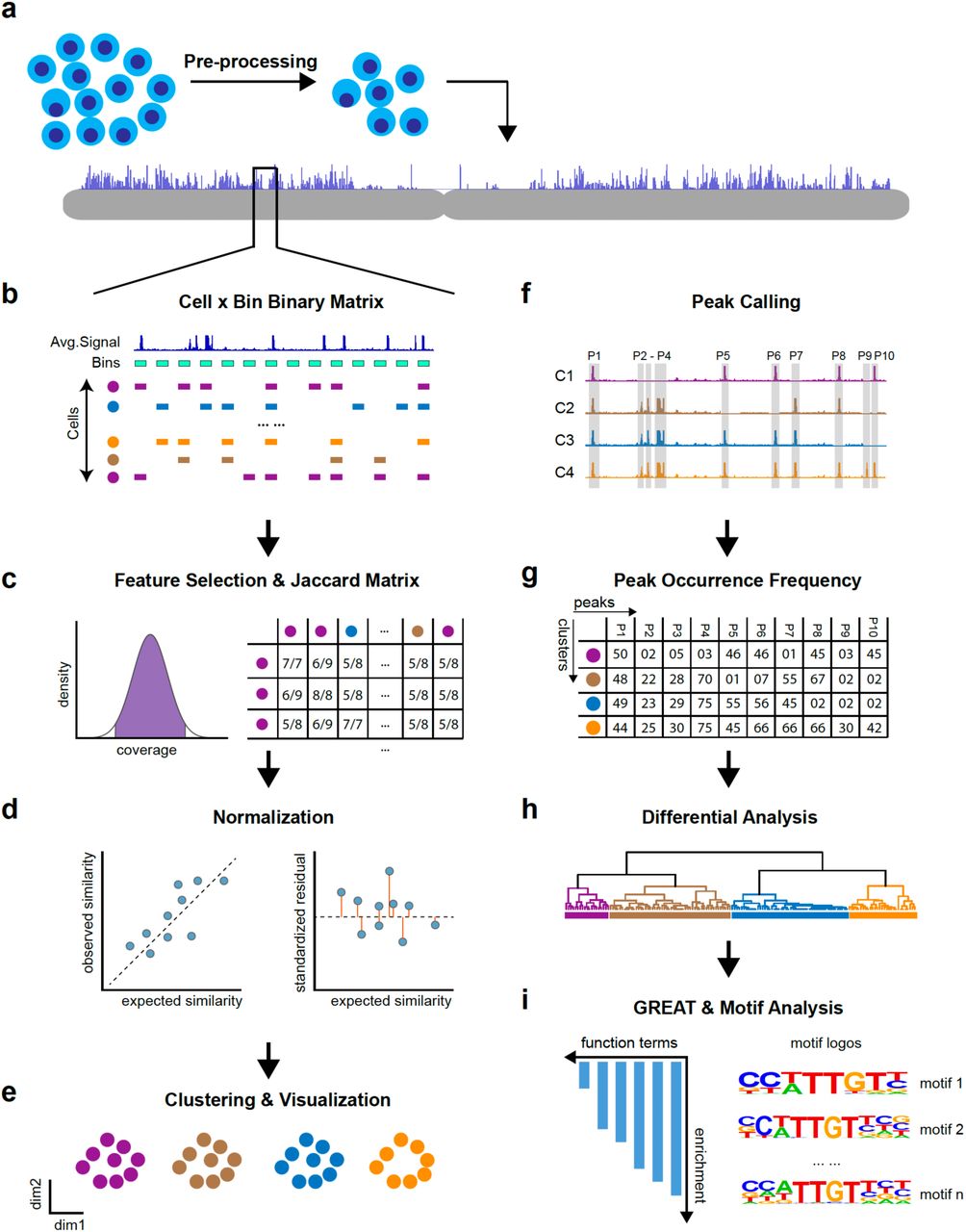
(a) Pre-processing: SnapATAC takes raw sequencing reads as input and aligns them to the reference genome followed by filtration of low-quality cells. (b) Cell-by-Bin Binary Matrix: the genome is segmented into uniform-sized bins and single cell profiles are represented as a binary matrix with “1” indicating a specific bin is accessible in a given cell and “0” denoting inaccessible chromatin or missing data. (c) Feature Selection & Jaccard Index Matrix: after filtering undesirable bins, the genome-wide cell-by-bin matrix is converted into a Jaccard index matrix by estimating similarity between cells in the basis of profile overlaps. (d) Normalization: Jaccard similarity matrix is normalized using a regression-based method to eliminate the read depth effect. (e) Clustering: using normalized matrix, cells of similar accessibility profiles are clustered together and visualized using t-SNE (t-Distributed Stochastic Neighbor Embedding) or UMAP (Uniform Manifold Approximation and Projection for Dimensionality Reduction). (f) Peak Calling: cells belonging to the same cluster are aggregated to create a representation of cell-type specific regulatory landscape for identification of candidate cis-regulatory elements de novo. (g) Peak Occurrence Frequency Matrix: the frequency (number of cells out of the total) of a peak occurring in each cluster is calculated. (h) Differential Analysis: differential analysis performed to identify cell-type specific regulatory elements. (i) GREAT & Motif Analysis: using cell-type specific regulatory elements, GREAT (Genomic Region Enrichment of Annotation Tool) analysis performed to predict the potential function of each cluster and motif analysis to reveal candidate master regulators that controls gene expression in each cell type.

The performance of SnapATAC is benchmarked against a variety of published scATAC-seq analysis methods, including chromVAR¹³, LSA⁸, Cicero¹⁵ and Cis-Topic¹⁴. To allow for evaluation of the clustering performance as a function of data sparsity, a set of simulated single-cell ATAC-seq datasets were generated by down sampling from 10 previously published bulk ATAC-seq datasets²¹ (Supplementary Table 1) with varying coverages, from 10,000 reads per cell (high coverage), to 1,000 reads per cell (low coverage) (Methods). The performance of each method in identifying the original cell types was measured by the normalized mutual index (NMI), which ranges from 0 for a level of similarity expected by chance to 1 for perfect clustering. This analysis shows that SnapATAC is the most robust and accurate method across all ranges of data sparsity (Fig. 2) (Wilcoxon signed-rank test, P < 0.01; Supplementary Fig. 3; Supplementary Table 2).

Figure 2. Validation of SnapATAC performance relative to alternative methods on simulated datasets.

Method comparison on 2,000 simulated single cell ATAC-seq data down sampled from 10 bulk ATAC-seq datasets with varying coverages. Mono: monocyte; Mega: megakaryocyte; GMPC: granulocyte monocyte progenitor cell; MPC: megakaryocyte progenitor cell; NPT: neutrophil; G1E: G1E; T cell: regulatory T cell; MEPC: megakaryocyte-erythroid progenitor cell; HSC: hematopoietic stem cell.

The superior performance of SnapATAC likely results from the fact that it considers all reads from each cell, not just a small fraction of reads that fall within peaks identified from aggregate signals. To test this hypothesis, the above analysis was repeated but only using off-peak reads. Consistent with this hypothesis, all cells were clustered perfectly (nmi=1.0; Supplementary Fig. 4). It is likely that these off-peak reads 1) overlap with “weak” elements that are not identified from the aggregate signals; 2) may be enriched for the euchromatin, which strongly correlate with active genes²² and vary considerably between cell types²³. Supporting this hypothesis, the density of 70% off-peak reads correlates strongly with compartment A defined in the particular cell types through genome-wide chromatin conformation capture analysis (i.e. Hi-C) (Supplementary Fig. 5). These observations suggest that the superior performance of SnapATAC with low-coverage datasets is, at least in part, due to that the off-peak sequencing reads in the scATAC-seq library contribute significantly for cell clustering.

To further assess the performance of SnapATAC, it is used to analyze a series of published single cell chromatin accessibility datasets representing a variety of sample types, and the results are compared to the original analysis. When applied to a set of 1,452 human cells corresponding to 10 distinct cell types¹³, SnapATAC successfully uncovered distinct cell populations with an accuracy of 0.95 (normalized mutual index) according to the cell labels, while the original method (chromVAR) failed to fully distinguish several blood cell subtypes (HL60, Blast, LMPP, LSC and Mono) (Fig. 3a; Supplementary Fig. 6a). Interestingly, SnapATAC divided K562 cells into two sub-clusters (Fig. 3a) (labeled as K562.2015, K562.2017), corresponding to the years (2015 and 2017, respectively) when the cells were grown and profiled (Supplementary Fig. 6b-c). In addition, GM12878 cells were also split into two separate clusters (GM12878.a and GM12878.b) (Supplementary Fig. 6b) that represent previously identified subtypes associated with differential NF-kB activity and B cell signaling⁵ (Supplementary Fig. 6d). Taken together, these results indicate that SnapATAC is a sensitive and accurate method to distinguish different cell types.

Figure 3. Validation of SnapATAC performance relative to alternative methods on published single cell ATAC-seq datasets.

(a) ChromVAR (top) versus SnapATAC (bottom) on scATAC-seq data from 11 human cell lines. Points are colored by cell types. Blast: acute myeloid leukemia blast cells; LSC: acute myeloid leukemia leukemic stem cells; LMPP: lymphoid-primed multipotent progenitors; Mono: monocyte; HL60: HL-60 promyeloblast cell line; TF1: TF-1 erythroblast cell line; GM: GM12878 lymphoblastoid cell line; BJ: human fibroblast cell line; H1: H1 human embryonic stem cell line. (b) POGODA2 (top) versus SnapATAC (bottom) on human Occipital Lobe scTHS-seq. Points are colored by identified cell types. (c) LSA (top) versus SnapATAC (bottom) on mouse prefrontal cortex sci-ATAC-seq dataset. Exc: excitatory neuron cells; Inc: inhibitory neuron cells; Opc: Oligodendrocyte precursor cells; Asc: astrocyte cells; Ogc: oligodendrocyte cells; Mgc: microglia cells. End: endothelial cells.

When applied to datasets from more complex tissues, SnapATAC also exhibits much improved performance over previous methods. Reanalyzing single-cell open chromatin profiles (scTHS-seq) from 6,008 human Occipital Lobe⁹, SnapATAC uncovered two additional inhibitory neuron subpopulations and four more excitatory subtypes corresponding to different layers (Fig. 3b) that were previously undetectable without incorporating single cell RNA sequencing data⁹. Similarly, when applied to a sci-ATAC-seq dataset comprising ~100,000 single cells from 13 adult mouse tissues⁸, SnapATAC revealed almost twice as many additional cell clusters as originally reported (Fig. 3c, Supplementary Fig. 7-10). For example, when applied to prefrontal cortex, SnapATAC identified 22 different populations including 12 excitatory neurons representing layer-specific subtypes, 5 inhibitory neuronal clusters including Sst, Vip, Pvalb, Sncg and Lamp5 subtypes, 1 oligodendrocyte cluster, 1 oligodendrocyte precursor cluster, 1 astrocyte cluster, 1 microglia cluster, 1 endothelial cell cluster (Fig. 3c, Supplementary Fig. 7-8). This improved cell-type resolution also holds true for other tissue samples tested (Supplementary Fig. 9-10). These results indicate that SnapATAC outperforms existing methods on complex single cell accessibility datasets.

In addition to the clustering performance, SnapATAC also demonstrates high computational efficiency and scalability. Benchmarked using simulated scATAC-seq data sets from 1,000 to 100,000 cells, the CPU-time of SnapATAC scales linearly and at a significantly lower slope than other methods. This difference is especially pronounced relative to topic modeling methods such as Cis-Topic, a probabilistic method that requires extensive parameter optimization for large dataset. Using the same computing resource, when applied to 100,000 cells, SnapATAC is nearly 160 times faster than Cis-Topic, reducing the time from 30 hours to 10 minutes (Table 1; Supplementary Fig. 11).

Table 1

Time taken for clustering using Cis-Topic and SnapATAC, as compared for different cell number N

A high-resolution cis-regulatory atlas of the secondary mouse motor cortex

The mammalian brain is composed of myriad highly specialized cell types and subtypes^{17, 24–27}, which presents a unique challenge for single cell chromatin accessibility analysis. As part of the BRAIN Initiative Cell Census Consortium²⁸, we have generated single nucleus ATAC-seq profiles from >60,000 individual cells from the secondary motor cortex (MOs) in the adult mouse brain (Fig. 4a). To our knowledge, this represents the largest single cell chromatin accessibility dataset yet published from a single tissue type. This dataset includes 2 biological replicates (Fig. 4b; Supplementary Table 3), each generated from pooled tissue of at least 15 mice to prevent potential artifacts such as dissection or batch effect. The aggregate signal showed high reproducibility between biological replicates (R > 0.95; Fig. 4b-c, Supplementary Fig. 12a-c) and significant enrichment for transcription start sites (TSS) indicating a high signal-to-noise ratio (Supplementary Fig. 12d-e). After filtering out the poor-quality nuclei using stringent criteria (Supplementary Fig. 13-14), we obtained a total of 64,795 nuclear profiles with an average of ~5,000 sequencing fragments per nucleus (Supplementary Table 4).

Figure 4. A high-resolution cis-regulatory atlas of the mouse motor cortex.

(a) Illustration of secondary motor cortex (MOs) in the adult mouse brain. (b) Genome browser view of snATAC-seq aggregated signals for two biological replicates. (c) Reproducibility of aggregate signals for two biological replicates (rho=0.96, P < 1e-10). (d) Two-dimensional visualization of SnapATAC clustering result. (e) Genome browser view of aggregate signal for each cluster at canonical marker genes. Mog is expressed in Oligodendrocyte cells; Apoe is expressed in Astrocyte cells; Pdgfra is expressed in Oligodendrocyte precursor cells; C1qb is expressed in Microglia cells; Slc17a7 is expressed in excitatory cells; Gad2 is expressed in inhibitory cells; Pvalb is strongly expressed in inhibitory Pvalb subtype; Vip is primarily expressed in inhibitory Vip subtype; Sst is expressed in inhibitory Sst subtype cells. Npy is expressed in inhibitory Lamp5 cells. (f) Cellular composition of cell types according to the SnapATAC clustering results. (g) Neuron versus non-neuron cell composition based on FACS sorting. (h) Imputed gene body accessibility level at marker genes for layer-specific excitatory neurons. (i) Dendrogram describing the taxonomy of neuronal subtypes.

SnapATAC identified and annotated the same 20 major clusters (Fig. 4d) from each biological replicate (Supplementary Fig. 15), indicating the robustness of the method. Based on gene body accessibility levels at canonical marker genes (Fig. 4e; Supplementary Fig. 16-17), the 20 clusters were classified into eight excitatory neuronal subpopulations (Snap25+, Slc17a7+, Gad1-; 50% of total nuclei), four inhibitory neuronal subpopulations (Snap25+, Slc17a7-, Gad2+; 10% of total nuclei), one oligodendrocyte subpopulation (Mog+; 9% of total nuclei), one oligodendrocyte precursor subpopulation (Pdgfra+; 5% of total nuclei), one microglia subpopulation (C1qb+; 7% of total nuclei), one astrocyte subpopulation (Apoe+; 13% of total nuclei), and additional populations of endothelial, somatic, and somatic muscle cells accounting for 6% of total nuclei.

The accuracy of these cell-type classification is supported by several lines of evidence. First, measurements of neuronal vs non-neuronal cell type abundance by Fluorescence-activated cell sorting (FACS) from the same samples are highly consistent with estimates from SnapATAC analysis (Fig. 4f-g; Supplementary Fig. 28). Second, the excitatory neuron subpopulations we identify show specificity for known cortical layer-specific marker genes and gradient transition between layers (Fig. 4h). Third, neuronal classification for each of the major cell population based on snATAC-seq data was in excellent agreement with previous annotations based on scRNA-seq²⁶ (Fig. 5a). All the major neuronal subpopulations identified from snATAC-seq can be matched to the scRNA-seq based classification of cell types in the mouse visual cortex. In addition, gene body accessibility for marker genes in each cluster correlated well with expression levels for corresponding genes and clusters (Fig. 5b and Supplementary Fig. 18). Taken together, these data show that snATAC-seq can dissect the cellular heterogeneity of mouse brain and classify cells in a way consistent with previous knowledge.

Figure 5. Comparison of neuron clusters with single cell RNA-seq.

(a) Two-dimensional visualization of single-nucleus ATAC-seq clusters of mouse secondary motor cortex. (b) Two-dimensional visualization of single neuron clusters from mouse frontal visual cortex using SMART-seq V4. (c) Comparison of imputed gene body accessibility and gene expression level at canonical marker genes. Gad2 is highly expressed in inhibitory neurons; Lamp5 is expressed in inhibitory Lamp5 subtype, excitatory L2/3 IT, L4 and L5 PT neurons; Sst is expressed in inhibitory Sst subtype; Pvalb is expressed in inhibitory Pvalb subtype.

Notably, one rare Sst neuronal subtype previously identified from scRNA-seq (Sst-Chodl in Fig. 5b) was not initially detected from snATAC-seq dataset. To examine whether iterative analysis could help tease out this rare population, SnapATAC was applied to 1,577 Sst nuclei, finding 9 distinct sub-populations including the Sst subtype (Sst.9), which accounts for less than 0.1% (52/64,795) of the total population profiled (Supplementary Fig. 19a-b). Based on gene accessibility and analysis of enriched transcription factor motifs (Supplementary Fig. 19d), Sst.9 most likely corresponds to Nos1 type I neurons (also known as Sst-Chodl). Applying SnapATAC to each of the other major neuronal cell types identified a total of 41 subtypes (Supplementary Fig. 20). To our knowledge, this represents the highest resolution of scATAC-seq analysis of a mammalian brain region. While the identity and function of these subtypes require further experimental validation, our results demonstrate the exquisite sensitivity of SnapATAC in resolving distinct neuronal subtypes with only subtle differences in chromatin landscape and gene expression patterns.

SnapATAC uncovers candidate cis-elements active in rare cell populations

A key utility of single cell chromatin accessibility analysis is to identify regulatory sequences in the genome. By pooling reads from nuclei in each cluster, cell-type specific chromatin landscapes can be obtained (Fig. 6a). Focusing on the major cell types described in Figure 4d, peaks of chromatin accessibility signals were determined in each cell cluster containing at least 500 cells, resulting in a combined total of 316,257 unique candidate cis-elements (Supplementary Table 5). Most notably, 56% (190,818/337,932) of these open chromatin regions are not detected in the analysis of bulk ATAC-seq data of the same brain region (Methods; Fig. 6b; Supplementary Table 6). We hypothesized that these open chromatin regions not detected in the bulk ATAC-seq analysis may represent those that are only accessible in minor cell populations. Supporting this hypothesis, nearly 80% of these elements were detected from only one cell cluster (Fig. 6c).

Figure 6. SnapATAC uncovers novel candidate cis-regulatory elements in rare cell types.

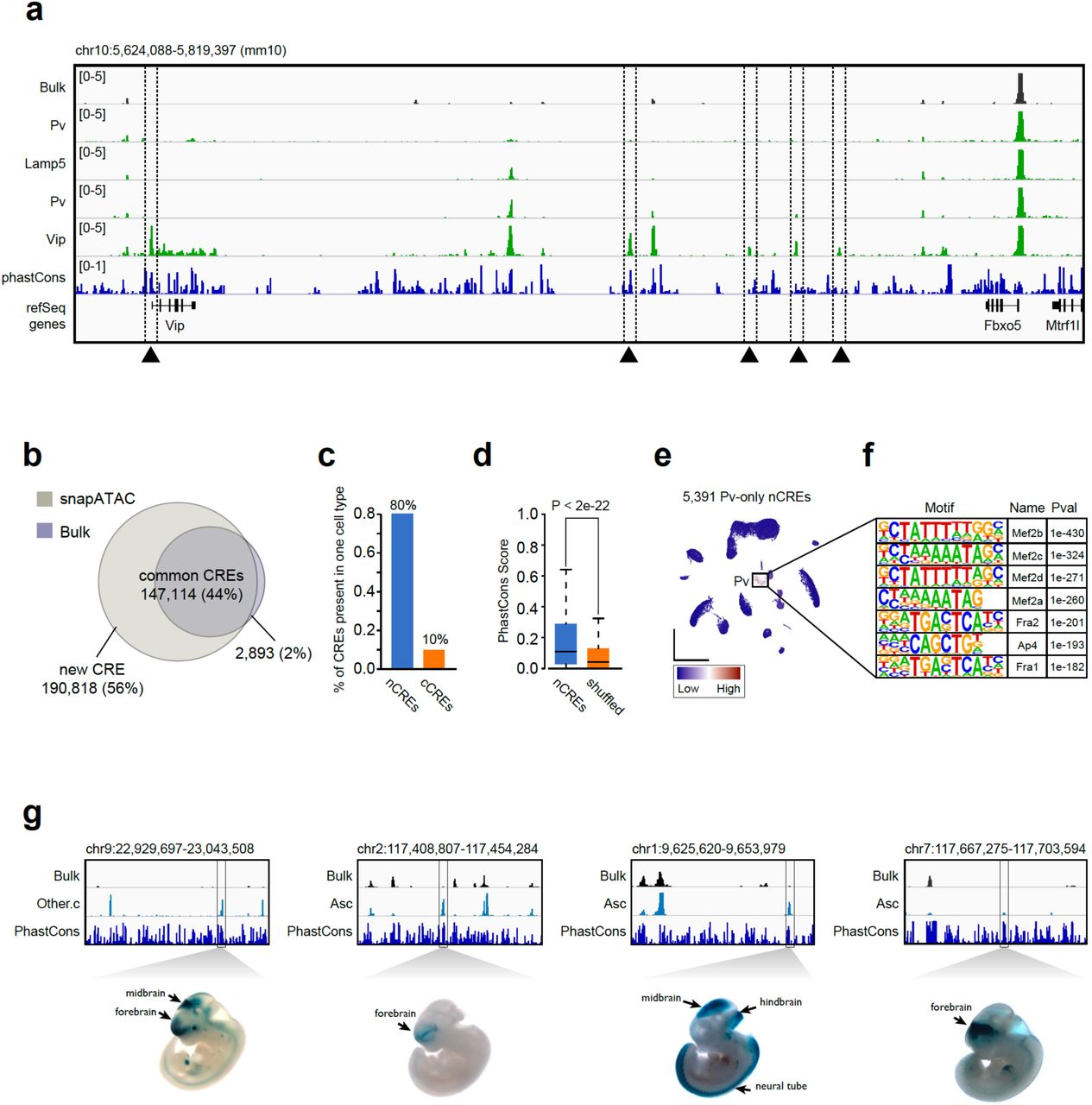
(a) Genome browser view of 20Mb region flanking gene Vip. Dash line highlighting five regulatory elements specific to Vip subtypes that are under-represented in the conventional bulk ATAC-seq signal. (b) Over fifty percent of the regulatory elements identified from 20 major cell populations are new compared to that of bulk ATAC-seq. (c) Eighty percent of new elements present in only one cell type. (d) Sequence conservation comparison between new elements and randomly chosen genomic regions. (e) 5,391 Pv-specific new elements are highly enriched in Pv subtypes. (f) Top seven motifs enriched in Pv-specific new elements. (g) Four new elements are tested positive using transgenic mouse assay according to VISTA database.

Several lines of evidence support that these additional open chromatin regions are functional elements, rather than technical noises. First, these sequences showed significantly higher conservation than randomly selected genomic sequences with comparable mappability scores (Fig. 6d). Second, these open chromatin regions display enrichment for transcription factor binding motifs corresponding to transcription factors (TFs) that play important regulatory roles in the corresponding cell types (Supplementary Table 7). For example, the binding motif for Mef2c is highly enriched in novel candidate cis-elements identified from Pvalb neuronal subtype (P-value = 1e-363; Fig. 7e-f), consistent with previous report that Mef2c is upregulated in embryonic precursors of Pv interneurons²⁹. Similarly, the binding motif for ETS-factor PU.1, a known transcription regulator of microglia³⁰, was highly enriched in the novel elements detected from microglia (P-value = 1e-2250) (Supplementary Table 7). Finally, the new open chromatin regions tend to test positive in transgenic reporter assays. Comparison to the VISTA enhancer database³¹ shows that enhancer activities of 256 of the newly identified open chromatin regions have been previously tested using transgenic reporter assays in e11.5 mouse embryos (Supplementary Table 8). 65% (167/256) of them drive reproducible reporter expression in at least one embryonic tissue, substantially higher than background rates (9.7%) estimated from regions in the VISTA database that lack canonical enhancer mark (manuscript under review)³². Here, we displayed four examples where elements were only present in rare population are tested positive in the brain function associating regions (Fig. 6g). It is important to note that this comparison only considers the in vivo enhancer function but does not validate the exact tissue-specificity because the current data cannot exclude the possibility of a regulatory element being an enhancer in other tissues.

Figure 7. Applying SnapATAC to other single cell modalities.

(a) A two-dimensional visualization plot of 14,963 DroNc-seq single-nucleus RNA-seq from adult frozen human hippocampus and prefrontal cortex. Nuclei are color-coded by cluster membership. exPFC: glutamatergic neurons from the PFC; GABA: GABAergic interneurons; exCA1/3: pyramidal neurons from the hip CA region; exDG: granule neurons from the hip dentate gyrus region; ASC: astrocytes; MGC: microglia; OGC, oligodendrocytes; OPC, oligodendrocyte precursor cells; NSC: neuronal stem cells; SMC: smooth muscle cells; END: endothelial cells. (b) A two-dimensional visualization plot of 2,784 methylomes form single neuronal nuclei in the human frontal cortex. (c) A two-dimensional visualization of single-cell Hi-C from HeLa S3 and HAP1 cells. (d) A two-dimensional visualization plot of H3K4me2 single cell ChIP-seq from ESCs and MEFs.

Extension of SnapATAC to other single cell epigenomics datasets

Although SnapATAC was designed to analyze single cell ATAC-seq data, it is also applicable to other sparse single cell datasets. To demonstrate this, SnapATAC was used to reanalyze a variety of published single cell epigenomics and transcriptomics datasets. When applied to a set of 14,963 sparse single nucleus RNA-seq (sNuc-seq) datasets from adult post-mortem human brain tissue³³, SnapATAC uncovered distinct clusters corresponding to all known major cell types (Methods; Fig. 7a; Supplementary Fig. 21-22). Sub-clustering of GABAergic neurons further identified 11 subtypes with distinct gene expression patterns (Supplementary Fig. 23), including two Sst, three Pv, three Vip subtypes and three clusters enriched for Lamp5 gene expression. Similarly, analyzing a dataset of 2,784 methylomes form single neuronal nuclei in the human frontal cortex²⁷, SnapATAC identified all the major and subtypes in excellent agreement with the previous classification (Fig. 7b; Supplementary Fig. 24). When applied to single cell H3k4me2 ChIP-seq data³⁴, SnapATAC correctly distinguished mouse embryonic stem cells (ESCs) from mouse embryonic fibroblasts (MEFs) cells (Methods; Fig. 7c). Finally, when used to analyze multiplexing single cell Hi-C³⁵, SnapATAC separates HeLa S3 from HAP1 cells (Methods; Fig. 7d). Taken together, these results show that SnapATAC can be used to process other single cell epigenomics datasets.

Conclusion & Discussion

In summary, SnapATAC is a comprehensive bioinformatic solution for single cell ATAC-seq analysis. The open-source software runs on commonly available and inexpensive hardware, making it accessible to any researcher using single-cell ATAC-seq data. Through extensive benchmarking using a variety of single cell chromatin datasets, SnapATAC outperforms existing methods substantially in both clustering accuracy and scalability. Although designed for analyzing single cell ATAC-seq datasets, SnapATAC can also be used to analyze a broad range of sparse single cell epigenomics data, such as single cell Hi-C, single cell ChIP-seq and single cell methylomes.

Applying SnapATAC to a new in-house dataset including >60,000 high quality single cell ATAC-seq profiles from mouse secondary motor cortex, led to a single cell atlas of candidate cis regulatory elements for this mouse brain region. The cellular diversity identified by chromatin accessibility is at an unprecedented resolution and is consistent with mouse neurogenesis and taxonomy revealed by single cell transcriptome data. Besides characterizing cell types, SnapATAC identifies candidate cis-regulatory sequences in each of the major cell types and infers transcription factors that control cell-type specific gene expression programs. Although this study primarily focused on the major cell types, additional neuronal subtypes can be identified through sub-clustering. To obtain a robust signal for each of the subtypes, would require substantially more cells and, more importantly, further anatomical, physiological, and functional experimental validation.

One of the most exciting features of SnapATAC is its ability to identify candidate cis regulatory elements active only in rare cell population. A large fraction (56%) of the candidate cis-elements identified using SnapATAC analysis of the mouse secondary motor cortex are not detected in bulk analysis. Most of these elements appear to be active in individual cell types that account for 1% or less of the total cell population. While further experiments to thoroughly validate the function of these additional open chromatin regions is still needed, the ability for SnapATAC to uncover cis-elements from minor cell types of a complex tissue will certainly greatly expand the catalog of cis regulatory sequences in the genome.

Data availability

Raw and processed data to support the findings of this study have been deposited to NCBI Gene Expression Omnibus with the accession number GSExxxxxx.

Code availability

The scripts and pipeline for the analysis can be found at https://github.com/r3fang/SnapATAC.

Author Contributions

This study was conceived and designed by R.F. and B.R.; Data analysis performed by R.F.; Tissue collection and nuclei preparation performed by J.L. and M.B.; Single nucleus ATAC-seq experiment performed by S.P., X.H. and X.W.; Tn5 enzymes synthesized and provided by A.M. and A.S.; Manuscript written by R.F. and B.R. with input from all authors.

Methods

1. SnapATAC Pipeline

1.1 Barcode Demultiplexing

Using a custom python script, we first de-multicomplexed FASTQ files by integrating the cell barcode into the read name in the following format: “@” + “barcode” + “:” + “original_read_name”.

1.2 Alignment & Sorting

De-multicomplexed reads were aligned to the corresponding reference genome (i.e. mm10 or hg19) using bwa³⁶ (0.7.13-r1126) in pair-end mode with default parameter settings. Alignments were then sorted based on the read name using samtools³⁷ (v1.9).

1.3 Fragmentation & Filtration

Pair-end reads were converted into fragments and only those that are 1) properly paired (according to SAM flag value); 2) uniquely mapped (MAPQ > 30); 3) with length less than 1000bp were kept.

1.4 Duplicates Removal

Sorted by barcode, fragments belonging to the same cell (or barcode) were automatically grouped together which allowed for removing PCR duplicates for each cell separately.

1.5 Snap File Generation

Next, using filtered and sorted bam file, we generated a snap-format (Single-Nucleus Accessibility Profiles) file which is hierarchically structured hdf5 file that contains the following sessions: header (HD), cell-by-bin accessibility matrix (AM), cell-by-peak matrix (PM), cell-by-gene matrix (GM), barcode (BD) and fragment (FM). HD session contains snap-file version, date, alignment and reference genome information. BD session contains all unique barcodes and corresponding meta data. AM session contains multiple cell-by-bin matrices of different resolutions (or bin sizes). PM session contains cell-by-peak count matrix. GM session contains cell-by-gene count matrix. FM session contains all usable fragments for each cell. Fragments are indexed for fast search which allows for generation of cell-type specific chromatin landscapes after clustering. Detailed information about snap file can be found in Supplementary Note 1.

1.6 Cell-by-Bin Count Matrix Generation

Using snap file, we next created cell-by-bin count matrices of different resolutions. The genome was segmented into uniform-sized bins and single cell ATAC-seq profiles were represented as cell-by-bin matrix with each element indicating number of open chromatin fragments overlapping with a given bin in a certain cell. A snap file allows for storing multiple cell-by-bin count matrices with different resolutions. For MOs snATAC-seq, we created snap file with 1kb, 5kb and 10kb resolution.

1.7 Barcode Selection

We next identified the high-quality barcodes based on the following criteria. 1) Total Sequencing Fragments (>1,000); 2) Mapping Ratio (>0.8); 3) Properly Paired Ratio (>0.9); 4) Duplicate Ratio (<0.5); 5) Mitochondrial Ratio (<0.1). We abandoned the use of reads in peak ratio as a metric for cell selection for two reasons. First, we found the reads-in-peak ratio is highly cell type specific. For instance, according to published single cell ATAC-seq, human fibroblast (BJ) cells have significantly higher reads in peak ratio (40-60%) versus 20-40% for GM12878 cells. Similarly, we found Glia cells overall have very different reads in peak ratio distribution compared to neuronal cells. We suspect this may reflect the nucleus size or global chromatin accessibility. Second, population-defined set of accessibility peaks are incomplete and are biased to the dominant populations. As shown in this study, for a complex tissue such as mammalian brain, we found over 50% of the peaks present in the rare populations are not identified from the aggregate signal of snATAC-seq. Therefore, we abandoned the use of reads in peak ratio for cell selection.

1.8 Bin Size Selection

Using the remaining cells, we sought to determine the optimal bin size based on the correlation between replicates. We recommend choosing the smallest bin size (or highest resolution) whose Pearson correlation between replicates is greater than 0.95. If there are no biological replicates available, we recommend splitting the cells into pseudo-replicates. In this study, we use 5kb unless noted.

1.9 Matrix Binarization

After choosing the optimal bin size, we found the vast majority of the items in the cell-by-bin count matrix is “0”, indicating either inaccessible (closed chromatin) or missing data. Among the non-zero elements, some items have abnormally high coverage (often > 200) perhaps due to alignment error. Therefore, we first removed the top 0.1% items of the highest coverage in the matrix before converting it into a binary matrix.

1.10 Feature Selection

We next filtered any bins overlapping with the ENCODE blacklist (http://mitra.stanford.edu/kundaje/akundaje/release/blacklists/) to prevent from any potential artifacts. Bins of exceedingly high coverage which likely represent the genomic regions that are invariable between cells such as housekeeping gene promoters were removed. We noticed that filtering bins of extremely low coverage perhaps due to random noise can also improve the robustness of the downstream clustering analysis. In detail, we calculated the coverage of each bin using the binary matrix and normalized the coverage by log10(count + 1). We found the log-scaled coverage obey approximately a gaussian distribution (Supplementary Fig. 25) which is then converted into zscore. Bins with zscore beyond ±2 were filtered before further analysis.

1.11 Jaccard Index Matrix

Next, we converted the genome-wide cell-by-bin matrix into a cell-by-cell similarity matrix by calculating the Jaccard index between every two cells in the basis of genome-wide profile overlaps. Usually, the number of cells is far smaller than number of bins, therefore, it immediately reduces the dimensionality and increase the scalability of the pipeline. However, the time for computing Jaccard matrix increases exponentially with cell number growth. To solve the problem of big data, 1) we first divided the cells into groups and calculated a sub Jaccard index matrix separately in parallel. For instance, given that there are 50,000 cells in total, we first split the cells into 10 chunks with each chunk containing 5,000 cells. Then we calculated the pairwise sub jaccard index matrix between every two chunks. Finally, we created the entire Jaccard index matrix by combining all sub Jaccard matrices. This allows for in-parallel computing. 2) To further speed up this process, instead of calculating a full Jaccard matrix by comparing every two cells, we calculated a partial Jaccard matrix by estimating the similarity between N cells with a subset of randomly chosen K cells (K << N) (k=2000 used in this study unless noted). We found that, without sacrificing the performance (supplementary Fig. 26), this can substantially improve the scalability of the pipeline, making it possible for processing millions of cells in the future.

1.12 Normalization

Theoretically, the entries of the Jaccard matrix M_ij, would reflect the true similarity between cell i and j. However, due to the differing coverage between cells, this becomes not the case. If there is a high sequencing depth of cell i, then M_ij will tend to have higher Jaccard index, regardless whether i and j is actually similar or not (Supplementary Fig. 1-2).

This can also be proved as below. Given 2 cells i and j and let X_i and X_j be the binary vector. The coverage of i and j is C_i = sum(X_i) and C_j = sum(X_j) (C_i>0, C_j>0), then let P_i = C_i/|X_i| and P_j = C_j/|X_j| where |X_i| and |X_j| is the number of bins. Then the expected Jaccard index between cell i and j is:

Because P_i * P_j > 0, then

Now it is obvious to see that the increase of either P_i or P_j will result in an increase of E_ij.

Here, we propose three different approaches to normalize Jaccard matrix, namely observed over expected (OVE), observed over neighbor (OVN) and iterative matrix balancing (ICE).

1.12.1 OVE: we first estimated the expected Jaccard index E_ij as described above, assuming cells have random profiles. We noticed that E_ij usually underestimates similarity for high-coverage cells, to adjust for this, we performed linear regression between expected E and observed M and used residuals as normalized matrix N. Residuals matrix N was then standardized for each cell.

1.12.2 OVN: the second approach estimated the expected cell-by-cell similarity using neighboring cells. In detail, for every pair of cells i and j, according to the coverage, we selected two groups of cells representing the k nearest neighboring cells for i and j with closest coverage. After removing common cells shared by , we next calculated the Jaccard matrix Jaccad between these two groups of cells, the average value of which was used as expected value to correct the bias in M_ij.

1.12.3 ICE: we also borrowed the idea of matrix balancing which is a technique commonly used in Hi-C matrix normalization. We adapted “normICE” function in HiTC R package which normalizes Hi-C matrix using matrix balancing algorithm that consists of iteratively estimating the matrix bias using the l1 norm.

To compare the performance of different normalization methods, we performed principle component analysis (PCA) against the normalized matrix and examined the degree of association between the first principle component and sequencing depth. Overall, a higher correlation indicates the dominate variance between cells is the read depth rather than the meaningful biological variance. For all the data sets we have tested, OVN and OVE overall shows a comparable performance (Supplementary Fig. 2), however, as OVE is substantially faster at least according to our implementation, therefore, we choose it as our final normalization method as used in this study. All the analysis is using OVE unless noted. But all three methods are implemented in SnapATAC package.

To further demonstrate the performance of the normalization, we applied it to previously published human scATAC-seq data from 10 cell lines¹³. The effect of normalization is clearly evident from inspecting the heatmap. Cell types that are difficult to distinguished in the original matrix become visibly distinct in the normalized matrix (Supplementary Fig. 2a-b). Further applying linear dimensionality reduction against both matrices, we found the first principal component of the raw matrix is strongly correlated with the coverage (rho=-0.90, P < 1e-10; Supplementary Fig. 2c), whereas the first dimension of the normalized matrix successfully distinguished BJ, TF from other cell types (rho=-0.04; Supplementary Fig. 2d).

We next tested it against other published datasets. When applied to human Occipital Lobe scTHS-seq⁹, the first principal component of normalized matrix separates neuronal from non-neuronal cells (Supplementary Fig. 2e). Similarly, when applied to the drosophila embryo sci-ATAC-seq data⁶, the first dimension now distinguished 4 major cell clades (Supplementary Fig. 2f). Together, all suggest that SnapATAC is able to adjust for the coverage bias.

1.13 Dimensionality Reduction

Like any other type of single-cell analysis, scATAC-seq contains extensive technical noise. To overcome this challenge, we performed Principle Component Analysis (PCA) to combine information across a correlated feature set hereby creating a mega-feature and exclude the variance potential resulting from technical noise.

1.14 Determining Significant Principle Components

It is both critical and challenging to decide how many principle components (PCs) to include for the downstream analysis. A variety of methods have been developed to identify optimal number of PCs. For instance, JackStraw³⁸ can specify significant components for PCA through permutation-based statistical test, however, this gets extensively time-consuming when cell number is large. Instead, we recommend using an ad hoc approach for choosing the optimal number of components. One approach as proposed by Sauret³⁹ to simplify look at the variance plot and find the “elbow” point. The other heuristic approach, we found also useful, is to plot every two pairs of PCs and simply look at the plot and choose number of PCs that stop separating cells.

1.15 Clustering

Using the selected significant PCs, we next calculated pairwise Euclidean distance between every two cells, using this distance, we created a k-nearest neighbor graph in which every cell is represented as a node and edges are drawn between cells within k nearest neighbors. Edge weight between any two cells are refined by shared overlap in their local neighborhoods using Jaccard similarity. Finally, we applied community finding algorithm Louvain to identify the ‘communities’ in the resulting graph which represents groups of cells sharing similar profiles, potentially originating from the same cell type. This method is also known as ‘Louvain-Jaccard’⁴⁰.

1.16 Visualization

We next project the high-dimension data into a 2D space using BH t-SNE⁴¹ implemented by Rtnse package or FI-tsne⁴² or UMAP⁴³ to visualize and explore the data. All three methods are integrated into SnapATAC package.

1.17 Cluster Annotation

To annotate the identified clusters, we next calculated the gene-body accessibility level for every cell and annotated the cluster based on the marker genes identified from previous single cell RNA sequencing. Note that clustering is unsupervised while annotation is a supervised procedure that requires expert knowledge. Recently, a method called Garnett⁴⁴ is developed to automatically annotate ATAC-seq clusters using single cell RNA-seq. To further enhance the structure of data and remove the noise, we adopted MAGIC⁴⁵ to smooth the gene accessibility signal.

1.18 Identification of Cis-Elements

Cells belonging to the same cluster are pooled to create ensemble signal for each of the cell type. This allows for identifying Cis-elements de novo from each of the clusters. MACS2⁴⁶ (version 2.1.2) was used for generating signal tracks and peak calling with the following parameters: --nomodel --qval 1e-2 -B --SPMR --call-summits.

1.19 Cell-by-Peak Accessible Matrix

Merging peaks identified from each cluster, we create a reference list of regulatory elements. Using this reference map, we next create a cell-by-peak count matrix.

1.20 Motif Analysis

We performed motif discovery using homer to infer the potential master regulator that control for gene expression in each of the cell types.

1.21 GREAT Analysis

We next performed Genomic Region Enrichment Analysis (GREAT) to predict the function of each cluster.

2. Analysis of simulated single cell ATAC-seq

First, we downloaded the alignment files (bam files) for ten bulk ATAC-seq experiment from ENCODE (Supplementary Table 1). From each bam file, we simulated 200 single cell ATAC-seq datasets by randomly down sampling to a variety of coverages ranging from 1,000 to 10,000 reads per cells. Using simulated single cell ATAC-seq datasets, we created a cell-by-bin matrix with 5kb bin size for SnapATAC clustering. Merging peaks downloaded from ENCODE for each experiment, we created a cell-by-peak matrix for LSA, Cis-Topic, Cicero and chromVAR clustering. Code used in this study can be found in Supplementary Note 2.

3. Analysis of published single cell ATAC-seq datasets

3.1 Analysis of scATAC-seq datasets from human cell lines

We obtained scATAC-seq count matrix from GEO (GSE99172). Analysis code used in this study is available in Supplementary Note 3.

3.2 Analysis of scTHS-seq datasets from human Occipital Lobe

The cell-by-peak matrix was generated and shared by Aerts Lab (http://scenic.aertslab.org/cisTopic/counts_Lake.Rds). Analysis code used in this study is available in Supplementary Note 4.

3.3 Analysis of sci-ATAC-seq datasets from mouse atlas

We downloaded processed data for each tissue from GEO (GSE111586) and generated the snap file with cell-by-bin matrix at 5kb bin resolution. Analysis code used in this study is available in Supplementary Note 5.

4. Tissue collection & Nuclei Perspiration

Adult C57BL/6J male mice were purchased from Jackson Laboratories. Brains were extracted from P56-63 old mice and immediately sectioned into 0.6 mm coronal sections, starting at the frontal pole, in ice-cold dissection media. The secondary motor cortex (MOs) region was dissected from the first three slices along the anterior-posterior axis according to the Allen Brain reference Atlas (http://mouse.brain-map.org/, see Supplementary S27 for depiction of posterior view of each coronal slice; dashed line highlights the MOs regions on each slice). Slices were kept in ice-cold dissection media during dissection and immediately frozen in dry ice for posterior pooling and nuclei production. For nuclei isolation, the MOs dissected regions from 15-23 animals were pooled, and two biological replicas were processed for each slice. Nuclei were isolated as described in previous studies^{27, 47}, except no sucrose gradient purification was performed. Flow cytometry analysis of brain nuclei was performed as described in Luo et al²⁷.

5. Tn5 transposase purification & loading

Tn5 transposase was expressed as an intein chitin-binding domain fusion and purified using an improved version of the method first described by Picelli et al⁴⁸. T7 Express lysY/I (C3013I, NEB) cells were transformed with the plasmid pTXB1-ecTn5 E54K L372P (#60240, Addgene)⁴⁸. An LB Ampicillin culture was inoculated with three colonies and grown overnight at 37°C. The starter culture was diluted to an OD of 0.02 with fresh media and shaken at 37°C until it reached an OD of 0.9. The culture was then immediately chilled on ice to 10°C and expression was induced by adding 250 µM IPTG (Dioxane Free, CI8280-13, Denville Scientific). The culture was shaken for 4 hours at 23°C after which cells were harvested in 2 L batches by centrifugation, flash frozen in liquid nitrogen and stored at −80°C. Cell pellets were resuspended in 20 ml of ice cold lysis buffer (20 mM HEPES 7.2-KOH, 0.8 M NaCl, 1 mM EDTA, 10% Glycerol, 0.2% Triton X-100) with protease inhibitors (cOmplete, EDTA-free Protease Inhibitor Cocktail Tablets, 11873580001, Roche Diagnostics) and passed three times through a Microfluidizer (lining covered with ice water, Model 110L, Microfluidics) with a 5 minute cool down interval in between each pass. Any remaining sample was purged from the Microfluidizer with an additional 25 ml of ice-cold lysis buffer with protease inhibitors (total lysate volume ~50ml). Samples were spun down for 20 min in an ultracentrifuge at 40K rpm (L-80XP, 45 Ti Rotor, Beckman Coulter) at 4°C. ~45 ml of supernatant was combined with 115 ml ice cold lysis buffer with protease inhibitors in a cold beaker (total volume = 160 ml) and stirred at 4°C. 4.2ml of 10% neutralized polyethyleneimine-HCl (pH 7.0) was then added dropwise. Samples were spun down again for 20 min in an ultracentrifuge at 40K rpm (L-80XP, 45 Ti Rotor, Beckman Coulter) at 4°C. The pooled supernatant was loaded onto ~10ml of fresh Chitin resin (S6651L, NEB) in a chromatography column (Econo-Column (1.5 × 15 cm), Flow Adapter: 7380015, Bio-Rad). The column was then washed with 50-100 ml lysis buffer. Cleavage of the fusion protein was initiated by flowing ~20ml of freshly made elution buffer (20 mM HEPES 7.2-KOH, 0.5 M NaCl, 1 mM EDTA, 10% glycerol, 0.02% Triton X-100, 100mM DTT) onto the column at a speed of 0.8ml/min for 25 min. After the column was incubated for 63 hrs at 4°C, the protein was recovered from the initial elution volume and a subsequent 30 ml wash with elution buffer. Protein-containing fractions were pooled and diluted 1:1 with buffer [20 mM HEPES 7.2-KOH,1 mM EDTA, 10% glycerol, 0.5mM TCEP) to reduce the NaCl concentration to 250mM. For cation exchange, the sample was loaded onto a 1ml column HiTrap S HP (17115101, GE), washed with Buffer A (10mM Tris 7.5, 280 mM NaCl, 10% glycerol, 0.5mM TCEP) and then eluted using a gradient formed using Buffer A and Buffer B (10mM Tris 7.5, 1M NaCl, 10% glycerol, 0.5mM TCEP) (0% Buffer B over 5 column volumes, 0-100% Buffer B over 50 column volumes, 100% Buffer B over 10 column volumes). Next, the protein-containing fractions were combined, concentrated via ultrafiltration to ~1.5 mg/mL and further purified via gel filtration (HiLoad 16/600 Superdex 75 pg column (28989333, GE)) in Buffer GF (100mM HEPES-KOH at pH 7.2, 0.5 M NaCl, 0.2 mM EDTA, 2mM DTT, 20% glycerol). The purest Tn5 transposase-containing fractions were pooled and 1 volume 100% glycerol was added to the preparation. Tn5 transposase was stored at −20°C.

To generate Tn5 transposomes for combinatorial barcoding assisted single nuclei ATAC-seq, barcoded oligos were first annealed to pMENTs oligos (95 °C for 5 min, cooled to 14 °C at a cooling rate of 0.1 °C/s) separately. Next, 1 µl barcoded transposon (50 µM) was mixed with 7 ul Tn5 (~7 µM). The mixture was incubated on the lab bench at room temperature for 30 min. Finally, T5 and T7 transposomes were mixed in a 1:1 ratio and diluted 1:10 with dilution buffer (50 % Glycerol, 50 mM Tris-HCl (pH=7.5), 100 mM NaCl, 0.1 mM EDTA, 0.1 % Triton X-100, 1 mM DTT). For combinatorial barcoding, we used eight different T5 transposomes and 12 distinct T7 transposomes, which eventually resulted in 96 Tn5 barcode combinations per sample⁷ (Supplementary Table 9).

6. Single-nucleus ATAC-seq data generation

Combinatorial ATAC-seq was performed as described previously with modifications^{5, 7}. For each sample two biological replicates were processed. Nuclei were pelleted with a swinging bucket centrifuge (500 × g, 5 min, 4°C; 5920R, Eppendorf). Nuclei pellets were resuspended in 1 ml nuclei permeabilization buffer (5 % BSA, 0.2 % IGEPAL-CA630, 1mM DTT and cOmpleteTM, EDTA-free protease inhibitor cocktail (Roche) in PBS) and pelleted again (500 × g, 5 min, 4°C; 5920R, Eppendorf). Nuclei were resuspended in 500 µL high salt tagmentation buffer (36.3 mM Tris-acetate (pH = 7.8), 72.6 mM potassium-acetate, 11 mM Mg-acetate, 17.6% DMF) and counted using a hemocytometer. Concentration was adjusted to 4500 nuclei/9 µl, and 4,500 nuclei were dispensed into each well of a 96-well plate. Glycerol was added to the leftover nuclei suspension for a final concentration of 25 % and nuclei were stored at −80°C. For tagmentation, 1 µL barcoded Tn5 transposomes^{7, 48} (Supplementary Table 9) were added using a BenchSmart™ 96 (Mettler Toledo), mixed five times and incubated for 60 min at 37 °C with shaking (500 rpm). To inhibit the Tn5 reaction, 10 µL of 40 mM EDTA were added to each well with a BenchSmart™ 96 (Mettler Toledo) and the plate was incubated at 37°C for 15 min with shaking (500 rpm). Next, 20 µL 2 × sort buffer (2 % BSA, 2 mM EDTA in PBS) were added using a BenchSmart™ 96 (Mettler Toledo). All wells were combined into a FACS tube and stained with 3 µM Draq7 (Cell Signaling). Using a SH800 (Sony), 20 nuclei were sorted per well into eight 96-well plates (total of 768 wells) containing 10.5 µL EB (25 pmol primer i7, 25 pmol primer i5, 200 ng BSA (Sigma)⁷. Preparation of sort plates and all downstream pipetting steps were performed on a Biomek i7 Automated Workstation (Beckman Coulter). After addition of 1 µL 0.2% SDS, samples were incubated at 55 °C for 7 min with shaking (500 rpm). We added 1 µL 12.5% Triton-X to each well to quench the SDS and 12.5 µL NEBNext High-Fidelity 2× PCR Master Mix (NEB). Samples were PCR-amplified (72 °C 5 min, 98 °C 30 s, (98 °C 10 s, 63 °C 30 s, 72°C 60 s) × 12 cycles, held at 12 °C). After PCR, all wells were combined. Libraries were purified according to the MinElute PCR Purification Kit manual (Qiagen) using a vacuum manifold (QIAvac 24 plus, Qiagen) and size selection was performed with SPRI Beads (Beckmann Coulter, 0.55x and 1.5x). Libraries were purified one more time with SPRI Beads (Beckmann Coulter, 1.5x). Libraries were quantified using a Qubit fluorimeter (Life technologies) and the nucleosomal pattern was verified using a Tapestation (High Sensitivity D1000, Agilent). The library was sequenced on a HiSeq2500 sequencer (Illumina) using custom sequencing primers, 25% spike-in library and following read lengths: 50 + 43 + 40 + 50 (Read1 + Index1 + Index2 + Read2)⁷.

7. Bulk ATAC-seq data generation

ATAC-seq was performed on 30,000-50,000 nuclei as described previously with modifications³. Nuclei were thawed on ice and pelleted for 5 min at 500 × g at 4 °C. Nuclei pellets were resuspended in 30 µl tagmentation buffer (36.3 mM Tris-acetate (pH = 7.8), 72.6 mM K-acetate, 11 mM Mg-acetate, 17.6 % DMF) and counted on a hemocytometer. 30,000-50,000 nuclei were used for tagmentation and the reaction volume was adjusted to 19 µl using tagmentation buffer. After addition of 1 µl TDE1 (Illumina FC-121-1030), tagmentation was performed at 37°C for 60 min with shaking (500 rpm). Tagmented DNA was purified using MinElute columns (Qiagen), PCR-amplified for 8 cycles with NEBNext® High-Fidelity 2X PCR Master Mix (NEB, 72°C 5 min, 98°C 30 s, [98°C 10 s, 63°C 30 s, 72°C 60 s] × 8 cycles, 12°C held). Amplified libraries were purified using MinElute columns (Qiagen) and SPRI Beads (Beckmann Coulter). Sequencing was carried out on a NextSeq500 using a 150-cycle kit (75 bp PE, Illumina).

8. Bulk ATAC-seq data analysis

ATAC-seq reads were mapped to reference genome mm10 using bowtie version 2.2.6 and samtools version 1.2 to eliminate PCR duplicates and mitochondrial reads. The paired-end read ends were converted to fragments. Using fragments, MACS2⁴⁶ version 2.1.2was used for generating signal tracks and peak calling with the following parameters: -q 0.01--nomodel -B --SPMR --keep-dup all. Library quality control for bulk ATAC-seq can be found in Supplementary Table 10.

9. Analysis of other single cell datasets

9.1 Analysis of single nucleus RNA-seq

We downloaded gene table from dbGaP under accession code phs000424.v8.p1. Analysis code can be found in Supplementary Note 6.

9.2 Analysis of multiplexing single cell Hi-C

The processed data is obtained from GEO with accession code GSE84920. Analysis code used in this study can be found in Supplementary Note 7.

9.3 Analysis of single cell ChIP-seq

We downloaded single cell matrix from https://pubs.broadinstitute.org/drop-chip/. Analysis code used in this study can be found in Supplementary Note 8.

9.4 Analysis of single nucleus methylome-seq

100kb-bin single nucleus methylome datasets were shared by Mukamel lab. We binarized the data by converting the methylation level into z-score and then set the bins with z-score less than −1.5 to 1.

Supplementary Figures

Figure S1. Comparison of normalization methods.

Figure S2. SnapATAC adjusts for coverage bias.

Figure S3. Validation of SnapATAC performance relative to alternative methods on simulated datasets.

Figure S4. SnapATAC identifies cell types using off-peak reads.

Figure S5. Off-peaks in single cell ATAC-seq library are enriched for euchromatin regions.

Figure S6. SnapATAC identifies potential batch effects and GM subtypes.

Figure S7. Gene accessibility level for selected markers of cell types expected in the pre-frontal cortex.

Figure S8. Sub-clustering identifies inhibitory neuronal subtypes in pre-frontal cortex sciATAC-seq data.

Figure S9. SnapATAC identifies additional cell types from published mouse cerebellum and kidney sci-ATAC-seq.

Figure S10. SnapATAC identifies additional cell types from LSA-defined major clusters.

Figure S11. SnapATAC outperforms existing methods in scalability.

Figure S12. Reproducibility between two biological replicates for mouse cortex at the level of aggregate signal.

Figure S13. Distribution of single cell quality control metrics for replicate 1.

Figure S14. Distribution of single cell quality control metrics for replicate 2.

Figure S15. Reproducibility of clustering result between two biological replicates.

Figure S16. Gene accessibility level for selected markers of major cell types expected in the mouse motor cortex.

Figure S17. Gene accessibility level for selected markers of inhibitory neuronal subtypes expected in the mouse motor cortex.

Figure S18. Comparison with scRNA-seq

Figure S19. Subdivision reveals rare Sst subtypes.

Figure S20. Subdivision reveals 37 neuronal subtypes.

Figure S21. Application of SnapATAC to single-nucleus RNA-seq.

Figure S22. Gene expression level for selected markers of major cell types expected in the human brain.

Figure S23. Sub-clustering of GABAergic neurons reveals subtypes in single nucleus RNA-seq.

Figure S24. Application of SnapATAC to single-nucleus methylome.

Figure S25. Bin coverage distribution.

Figure S26. Partial Jaccard index matrix using different number of features.

Figure S27. Illustration of secondary motor cortex dissection.

Figure S28. Gating strategy for nuclei sorting.

Supplementary Tables

Table S1. Ten bulk ATAC-seq used for simulating single cell ATAC-seq datasets

Table S2. Comparison of clustering performance of five methods on simulated datasets

Table S3. Alignment statistics for mouse motor cortex single nucleus ATAC-seq library

Table S4. Metadata of mouse MOs single neuron ATAC-seq

Table S5. A merged list of cis-Regulatory elements from all cell clusters

Table S6. Cis-Regulatory elements identified using bulk ATAC-seq

Table S7. Motifs enriched for cell-type specific elements

Table S8. VISTA enhancers overlapping with new cis-elements

Table S9. Barcode indices used for single nucleus ATAC-seq experiment

Table S10. Alignment statistics for mouse motor cortex bulk ATAC-seq library

Acknowledgements

We thank D. Gorkin, R. Raviram, J. Hocker and X. Zhou for proofreading and suggestions for the manuscript. We thank S. Kuan for sequencing support. We thank O. Poirion, C. Zhang and B. Li for Bioinformatics support. We thank F. Xie for sharing processed single nucleus methylome data. We thank C. O’Connor and C. Fitzpatrick at Salk Institute Flow Cytometry Core for sorting of nuclei. This study was funded by U19MH114831.