

Abstract
Perception is an active process involving continuous interactions with the environment. During such interactions neural signals called corollary discharges (CDs) propagate across multiple brain regions informing the animal whether itself or the world is moving. How the interactions between concurrent CDs affect the large-scale network dynamics, and in turn help shape sensory perception is currently unknown. We focused on the effect of saccadic and body-movement CDs on a network of visual cortical areas in adult mice. CDs alone had large amplitudes, 3-4 times larger than visual responses, and could be dynamically described as standing waves. They spread broadly, with peak activations in the medial and anterior parts of the dorsal visual stream. Inhibition mirrored the wave-like dynamics of excitation, suggesting these networks remained E/I balanced. CD waves superimposed sub-linearly and asymmetrically: the suppression was larger if a saccade followed a body movement than in the reverse order. These rules depended on the animal’s cognitive state: when the animal was most engaged in a visual discrimination task, cortical states had large variability accompanied by increased reliability in sensory processing and a smaller non-linearity. Modeling results suggest these states permit independent encoding of CDs and sensory signals and efficient read-out by downstream networks for improved visual perception. In summary, our results highlight a novel cognitive-dependent arithmetic for the interaction of non-visual signals that dominate the activity of occipital cortical networks during goal-oriented behaviors. These findings provide an experimental and theoretical foundation for the study of active visual perception in ethological conditions.
Introduction
Corollary discharges (CDs) are copies of motor commands that do not themselves produce body movements, but inform brain regions on whether the animal or the world is moving1-4. These signals are found ubiquitously in the animal kingdom2 and it is increasingly understood they profoundly impact the dynamics of several brain regions, affecting sensory perception as well5-8. During ethological behaviors multiple CDs concurrently propagate across neural networks1. However in traditional approaches CDs have been either isolated one at a time for experimental convenience or labelled as uncontrolled variability and abolished with anesthetized preparations or behavioral paradigms that minimize motor components. Accordingly, how CDs interact with each other and how these interactions affect sensory perception during goal-directed behaviors is currently unknown.
We addressed these questions in the visual cortex of awake mice, which has served as a model system for two very well-studied CDs, those for saccadic eye movements9-14 and for body movements15-20. We first characterized the large-scale dynamics of the CDs analyzed individually or when interacting with each other and with visual signals. Then we examined the cognitive dependence of the found properties and their relevance to perception by studying the animals’ behavior in a visual discrimination task.
Results
Mice (n=15) were trained in a two-alternative forced choice (2AFC) orientation discrimination task (Fig. 1a,b, Extended Data Fig. 1a) with automated setups featuring self head-fixation21. Head-fixed mice made frequent voluntary saccadic eye movements mostly in the nasal-temporal direction22 (Fig. 1c, Extended Data Fig. 1d, Supp. Video 1) and preferentially after the stimulus presentation (in the open-loop period, OL, Fig. 1a,d), possibly reflecting a task-related exploration of the visual stimuli. This saccadic pattern emerged with training, with naïve animals making significantly fewer exploratory eye movements despite being shown the same visual stimuli – more salient given their novelty (Extended Data Fig. 1b). Animals reported their choice by rotating a wheel with their front paws23 (Fig. 1a,b). Wheel rotations – from hereafter denoted ‘body movement’ – were associated with more general movements of the trunk, tail, snout, whiskers, etc., (Supp. Video 2).

Corollary discharges during decision making. a) Setup and task structure. b) Psychometric curve, example mouse; black line, fit (Methods); gray dots, data. c) Probability of saccade landing positions. White square, session-average eye resting position. d) Probability of body movements (top) and saccades (bottom) during the trial, in excitatory (black; n=10) and PV (dark blue; n=5) mice; error bands, s.e. e) Visual field sign maps for excitatory and PV mice (n=10 and 5). f) Event related responses. Rows 1-4: saccade, wheel, simulated saccade and stimulus, across corresponding ROIs (columns) for excitatory (black) and PV (blue) mice. Max amplitude of saccadic response: 2.5±0.4 (Exc) and 2.1±0.3 (PV), %dF/F ± s.e.; t-test comparing to stimulus response, p<10−4. FWHM 0.56±0.06s and 0.46±0.08s (t-test PV vs Exc, p=0.38). Body-movement response: peak 2.2±0.2 and 2.5±0.4; larger than stimulus response, t-test p<10−4 and 0.005; FWHM 0.83±0.07s and 0.94±0.11s (t-test p=0.4). Peak simulated saccade response: 0.53±0.04% and 1±0.24%. Peak stimulus response: 0.57±0.05% and 0.9±0.2%. Insets: saccade (black) and body movement (red) velocities for each event, for excitatory mice. g) Peak response maps: average normalized responses for each event (rows) at its corresponding peak time, for excitatory (1st column) and PV (2nd column) mice (Methods). Gray area contours as in (e). White crosses indicate ROI centers used in (f), Extended Data Fig. 10 j-n.
During behavior we imaged responses from excitatory neurons in a large network of visual cortical areas (n=10 mice, Fig. 1e, Extended Data Fig. 1c, Methods). Notably, responses to isolated saccades were about four times larger than contrast responses (Fig. 1f), even in the V1 retinotopic location of the stimulus (Fig. 1f-g). Saccades strongly activated medial V1 and the medial part of the dorsal visual stream (areas PM, AM, A, Fig. 1g, Extended Data Fig. 2a,b,g) – regions implicated in the magnocellular hypothesis of saccadic suppression14,24 – anterior visual-parietal areas25 (Extended Data Fig. 2i,j) and partially-imaged somatosensory areas26. After about half a second of transient increase, the response was followed by a delayed suppression below baseline activity (Fig. 1f). The overall dynamics could be described in terms of a global spatial pattern whose amplitude was modulated over time, i.e. a standing wave of activity (Extended Data Fig. 3a, Methods). Deviations from the wave dynamics (residuals of a singular-value decomposition, Methods) revealed a small but significant response in motion sensitive areas27 (i.e. RL, AL and LM, Extended Data Fig. 3c) with peak amplitude about 1.4 seconds after the onset of the saccade, possibly linked to a reafferent retinal signal, i.e. a sensory input induced by the eye movements.

Correlations between pupil dilation, performance and cortical states. a) Pupil area changes after stimulus onset for correct (C), incorrect (I) and timeout (TO) choices. b) Iso-contour lines (10th percentile) of C/I/TO trial distributions in pupil space (Methods). c) Performance in different regions of pupil space. Contour lines (10th percentile) for trials with high (red) and low (cyan) DR. d) Performance in different regions of dF/F space (Methods). Contour lines for high and low DR (10th percentile). e) Performance in high vs low DR trials (population average for sessions with >60% C and <20% TO, 72±1% correct in high DR; 65±2% in low DR, s.e., difference of the means across animals, p=0.02, Wilcoxon, n=12). f) Pupil dilations for interacting CDs. Red and blue dots, high and low DR. g) Neural responses for quadrants 1-4 in the pupil space (f). Inset: pupil modulation for the 4 quadrants in (f). h) 95th percentile contour lines of C/I/TO distributions in the dF/F space (d), for high, average, and low DR conditions.

Stimulus-CD and CD-CD interactions. a) Left: stimulus-saccade interaction for excitation (black) in stimulus ROI and its linear prediction (red), i.e. the sum of stimulus and jittered saccade responses. Horizontal double arrow, jittering window (Methods). Right: spatial map of activation at time of peak response. Peak response amplitude is 3.8x larger than the contrast response (t-test, p<10−4; n=10). FWHM: 0.5±0.04s s.e. same as for isolated saccades, t-test p=0.5. b) Left: same as in (a), for stimulus-body movement interactions in stimulus ROI. Peak response is 3x larger than contrast response (t-test, p<10−4). FWHM: 0.83±0.09s same as for isolated body movements, t-test p=0.98. c) Responses to interacting CDs in saccade ROI for excitatory mice. Left: saccade-body movement interaction and linear prediction (red; Methods). Peak responses are 1.2x and 1.3x larger than for isolated saccades and body movements (t-test, p=0.2 and 0.01), but smaller than their linear sum (t-test, p<10−3). Middle: spatial response at time of peak amplitude for interacting CDs in excitatory mice. Right: suppressive response at time of peak suppression. d) GLM sequential fitting: average dF/F aligned to stimulus onset in trials with CD-CD interactions (black), gray band CI, example mouse. Model responses: stimulus (green), stimulus + isolated CDs (red), stimulus + isolated CDs + nonlinear CD interaction (blue). e) Average CD-CD interaction kernel for excitatory mice (n=8) in regions of max suppression (g). Masked black squares if n<5 mice (Methods). Red dots, maximum suppression for individual animals; large circle for population average (lag τb=tobserv-tb=0.74±0.06s, τe=0.16±0.03s, one outlier omitted, error bars smaller than circle size). f) Top center, illustration of relative lag Δτ = τb - τe and time to nearest movement Δt = min(τe, τb), τe > 0, τb > 0. Top left and right – schematic of kernel elements with fixed Δτ and Δt, in the same color. Left. Maximum suppression as a function of Δτ. Population average, black line (CI, dark gray); individual animals, light gray. Asterisks, values different from minimum of average curve (Δτ=0.5, diamond) (U-test, α=0.05). Average Δτmin across animals: 0.58±0.05s. Right. Maximum suppression as a function of Δt, same colors as (f). Average Δtmin across animals, 0.16±0.03s. g) Spatial distribution of nonlinear CD-CD component at time of maximum suppression (red circle in (e)).
However, reafference was not a significant contributor to the overall response pattern. Indeed, the onset of neural activity preceded the onset of saccades by 110ms (-110±20ms, s.e.), with the spatial profile of the activation already matching that of the post-saccadic response (Extended Data Fig. 2c). Nasal or temporal saccadic eye movements did not produce significantly different activations (Extended Data Fig. 2d), as it should be expected by reafferent signals1,2. Furthermore, in experiments where we jittered the stimuli on the screen with displacement vectors and velocities drawn from the distribution of actual saccades (simulated saccades28, Extended Data Fig. 1e, Methods), responses had smaller amplitudes than saccadic ones and were localized in motion-sensitive areas27 (Fig. 1f,g). Finally, saccadic responses in the absence of contrast stimuli (Methods) and of behavioral task (“blanks”) were comparable to those evoked in the presence of contrast stimuli, although the delayed suppression was significantly reduced (Extended Data Fig. 4a-c).

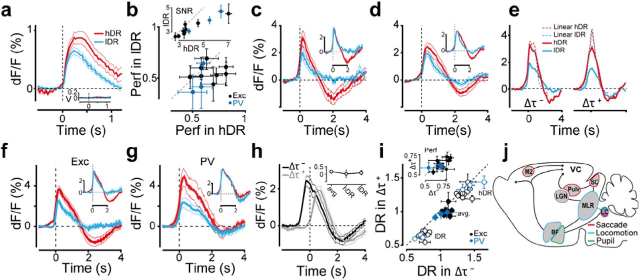
DR-dependent modulation of stimulus and CDs. a) Responses to isolated stimulus in high (red) and low (blue) DR for excitatory mice. Inset: velocities of saccade and body movements for corresponding conditions. b) Performance in high and low DR for trials with isolated stimuli (Wilcoxon p = 0.04, n=11). Only sessions with >50% performance and <30% timeout rate are included. Inset: signal to noise ratio for corresponding trials (Wilcoxon p=0.001). c) Responses to isolated saccades in high and low DR. Inset, responses normalized to high/low peak ratio. d) Responses to isolated body movements in high and low DR. Inset as in (c). e) Left: average dF/F during interactions with relative lags Δτ−: -700ms<Δτ<-300ms (saccade before body movement, Fig. 2f) in high and low DR. Dotted lines show predictions of the linear part of the GLM, red box Fig. 2d. Right: same as left, but with relative lags Δτ+: 300<Δτ<700ms (saccade after body movement). Responses are aligned to the time of saccade. f) Responses to interacting CDs in high and low DR. Inset, as in (c). g) Same as (f) for PV mice. h) Response to interacting CDs at different lags, aligned to saccade time. Inset, fractional ratio of Δτ− and Δτ+ responses averaged across all trials (“avg.” label), and in high and low DR. i) DR in Δτ− is larger than in Δτ+ in hDR, on average, and in lDR conditions (Wilcoxon on means across all trials: all DR p = 0.002, h-DR p = 0.02, l-DR p<10−4; and p<10−4 for session means in each condition). Inset: average performance in Δτ− versus Δτ+ (Wilcoxon p=0.007 across all trials). j) Schematic of the circuits controlling saccades, body movements, and pupil-related arousal states: VC, visual cortex. Pulv, pulvinar. SC, superior colliculus. LGN, lateral geniculate nucleus. MLR, mesencephalic locomotor region. LC, locus coeruleus. BF, Basal forebrain. M2, secondary motor cortex.
The second corollary discharge we examined was related to body movements16, also typically occurring after the stimulus onset (Fig. 1d). Consistent with studies on locomotion5,15, body movements elicited large-amplitude responses, about three times larger than responses to visual stimuli (Fig. 1f,g). They localized in medial V1 and dorsal stream areas (Fig. 1g), such as the posterior parietal cortex (A, anterior-RL, and AM25), and the hind-paw somatosensory areas26. Similar to saccades, responses emerged before the initiation of the wheel rotation (-237±31ms, s.e.; n=10; Extended Data Fig. 2c) reflecting either a pre-motor preparatory component8,19,29, or stereotypical undetected movements preceding wheel rotations. After about half a second of transient increase, responses were followed by a delayed suppression (Fig. 1f,g). Also in this case, the overall dynamics could be well summarized in terms of a standing wave of activity (Extended Data Fig. 3a). An analysis of the residuals from the wave dynamics identified a small but significant response in motion-sensitive areas (Extended Data Fig. 3c), likely related to the stimulus motion induced by the wheel rotation (closed-loop period, CL, Fig. 1a).
Inhibitory activity (PV-cre line, n=5) approximately mirrored excitatory activity both for saccades and body-movements20,30,31. Responses were ∼2.5× and ∼2.9× larger than those evoked by visual stimuli26 (Fig. 1f,g) with an amplitude increase preceding saccadic and body movements (Extended Data Fig. 2c). Both saccades and body movements had a delayed suppression and the overall response in blank conditions resembled those of excitatory neurons (Extended Data Fig. 4a-c). Responses were widespread32 with a similar cortical localization as excitatory neurons (Fig. 1g). The overall dynamics was also consistent with a standing wave of activity (Extended Data Fig. 3a).
In summary, saccadic and body movement responses were consistent with standing waves of activity and were several folds larger than contrast responses, with spatially distinct activation patterns (Extended Data Fig. 2e,f). Both CDs were characterized by non-sensory components emerging before the movement, and had a delayed suppressive response that could not be fully explained by an overlapping slow intrinsic signal26,33-35 since it was not observed in response to retinal inputs (Fig. 1f, stimulus and simulated saccades). There was a strong similarity in the spatial and temporal activity patterns of PV and excitatory populations30, with excitation and inhibition (E-I) seemingly balanced during saccadic and body-movement CDs.
Saccades and body movements often occurred in close temporal proximity and soon after stimulus onset (Fig. 1d, Extended Data Fig. 1b), giving us the opportunity to examine the properties of the stimulus-CD and of the CD-CD interactions. For stimulus-CDs interactions we calculated average responses in trials when saccades or body movements occurred in close temporal proximity with the stimulus onset (Methods). A prominent feature was a significant larger peak response amplitude than for isolated visual responses (Fig. 2a,b; Extended Data Fig. 5a,b). The duration of stimulus-CD response was comparable to that of isolated saccade or body-movement CDs. Moreover, the spatial distribution also resembled that of saccades or body movements (Extended Data Fig. 5c). An analysis of linearity (GLM, Methods) revealed that the saccade and stimulus interaction was supralinear, while the body-movement and stimulus interaction was sub-linear when stimulus and CD coincided, but it was supralinear when the CD followed the stimulus15 (Extended Data Fig. 6). When saccadic and body movement CDs interacted within short temporal windows, peak response amplitudes were larger than for isolated CDs but significantly smaller than their linear sum (Fig. 2c; Extended Data Fig. 7a-f). We confirmed this was not a result of GCaMP-signal saturation (Extended Data Fig. 7i). Responses also had a strong delayed suppression (Fig. 2c), largest at 2.2±0.2s from the time of interaction. The spatial pattern of the peak CD-CD interaction was mostly a superposition of isolated CDs and it was distinct from the spatial pattern of the delayed suppression, which was more uniformly localized in anterior regions (Extended Data Fig. 7g,h). The sublinear summation was well captured by an overall suppressive component in a GLM-derived interaction kernel (Fig. 2d-g, Methods). Notably, the strongest suppressive interaction occurred when a saccade happened after a body movement (Fig. 2e-f; Extended Data Fig. 8a,c). Similar to the spatial pattern of the peak CD-CD interaction, the nonlinear suppressive component at the time of its maximum was broadly distributed across visual areas, with the peak suppression localized similarly to the isolated saccadic response (Fig. 2g). In PV mice the CD-CD interaction was also suppressive and asymmetric, but less pronounced than for excitation (Extended Data Fig. 8b,d-g). In summary, the contrast response was overshadowed by the interacting CDs, resulting in a response profile similar to that of CDs in isolation. Interactions were nonlinear, and depended on the lag between stimulus onset and saccade or body movement. The CD-CD interaction was primarily suppressive, with an asymmetry relative to the order of the CDs. Interacting responses were localized in the medial part of V1 and in the medial-anterior dorsal stream areas, being more prominent in excitatory neurons than in PV cells.
Next, we examined how the summation dynamics between CDs and with visual stimuli might affect the processing of visual information and consequently the animal’s sensory perception. We started by formulating a simple hypothesis for the previously described temporal asymmetry in the interactions, reasoning that the order of motor execution (saccade or body movement first) could link to learned behavioral patterns in trained mice. For example, a mouse highly engaged in the task could first visually explore (saccade) and then make a wheel movement, with the reverse order being more typical of less engaged animals. Since cognitive-state changes (i.e. task engagement, attention, arousal, etc.) are known to correlate with changes in cortical states36-39, the asymmetry would emerge because movements with different temporal orders occur in different cortical states. Consistent with this hypothesis, also the processing of CDs in isolation – and of visual signals – should depend on cortical states and correlate with performance, as a reflection of changes in cognitive states. To examine these possibilities we analyzed differences in cognitive states38 using pupil dilation as a biomarker38, evaluated visual perception through the animal’s ability to discriminate orientations in the 2AFC task, and measured the dynamics of cortical states via quantifiers derived directly from the neural responses.
To characterize the link between cognitive states, performance and cortical states, we pooled across all CD interactions and defined a space of pupil baseline and area change, (Fig. 3a-c, Extended Data Fig. 2h, Methods), associated to tonic and phasic changes in pupil dilations31,40. As expected, the animal’s performance varied across regions of this pupil space, with gradual increase in performance for larger pupil area (Fig. 3b,c), and with a trend for peak performance at intermediate values of area change (Fig. 3c), in agreement with Yerkes-Dodson inverted U-curve41. Notably, correct trials extended to regions of the largest pupil area, more so than incorrect trials, while time-out trials densely clustered in the region of small pupil area, suggesting an overall reduction in task engagement8 (Fig. 3b). To quantify differences in cortical states, we relied on two measures. First, we defined a dynamical range index (DR) that measures the standard deviation of the neural response throughout a trial (Methods). Large-amplitude CDs could drive high DR values, but CDs were neither consistently sufficient nor necessary for high DR states (Extended Data Fig. 9a, Fig. 3f,g). This index reflected either changes in cortical states following modulations in the animal’s cognitive state36,42 or undetected sensory-motor components. The former interpretation was supported by the wider spread of trials with high DR in the pupil space (Fig. 3c), also accompanied by higher performance (Fig. 3d,e), suggesting increased arousal or engagement in high DR states. Using the stimulus-locked change in the neural response as a second measure of cortical state (Methods), we observed the highest performance in trials with the largest changes (Fig. 3d). Overall, this measure was an informative regressor of the trial choice, with correct, incorrect, and time-out trials characterized by progressively smaller amplitude changes (Fig.3h). This trend was observed also when splitting trials into high and low DR groups, indicating that the neural-to-behavioral correlation was observable on a trial basis and persisted across a broad range of cortical and cognitive states (Fig. 3h). In summary, when analyzing pupil dilation, neural responses and task performance, we observed a significant correlation between psychometric and neurometric parameters with co-variability in cognitive, performance, and cortical states.
As hypothesized, cortical-state changes affected visual responses and CDs, both when considered in isolation or as interacting. The amplitude of the stimulus-evoked response in isolation from other movements (Methods), was larger and had a higher signal-to-noise ratio43 (Methods) in high DR states, when performance was also higher (Fig. 4a,b). Responses to isolated saccadic and body movements remained space-time separable (standing waves) across DR states, with the peak amplitude and the delayed suppression both enhanced in high DR states, in accord with a multiplicative gain modulation5,6 (Fig. 4c,d; Extended Data Fig. 9). A similar dependence on dynamical range and performance was observed in CD interactions (Fig.4e-g). In particular, the non-linear suppression was smaller in high DR states, suggesting increased functional independence between CDs, with interactions better described as a linear sum of isolated CDs (Fig. 4e). Notably, although the E-I ratio was on average balanced in isolated and interacting CDs (Fig. 4f,g), in trials with high DR the initial part of the response was multiplicatively scaled both for E and I activations, but in the later part, E was further reduced than I, skewing the ratio toward an overall response suppression (Fig. 4f,g). A possible explanation relates to the phasic and tonic changes in pupil area that had multiplicative and subtractive effects on the interacting responses (Fig. 3f,g, quadrants 2,3 and 1,4 respectively). Hence a cortical-state dependent recruitment of the brain circuits involved in the pupil control could underlie the late E-I imbalance20,31,40,44-47. Regarding the temporal asymmetry in CD interactions, both dynamical range and performance were significantly larger when saccades happened before body movements than in the reverse order (Fig. 4h,i). This asymmetry was invariant with respect to cortical states and observed on a trial basis, i.e. when grouping trials into high or low DR states (Fig. 4i). Together these considerations support the proposed hypothesis that changes in cognitive state associated to higher performance and larger DR values, better correlate with a behavioral pattern where visual exploration precedes body movements. Further support to this interpretation comes from the observation that saccades after stimulus onset, but not those preceding it, correlated with higher performance (Extended Data Fig. 6e). According to a mechanistic interpretation, the functional circuits recruited by the CDs are differentially modulated by the animal’s cognitive state36-38. This is possible via cholinergic48,49 and noradrenergic neuromodulatory systems known to be robustly activated by these CDs and implicated in the control of arousal and attention50-52 (Fig. 4j). This mechanistic view suggests a simple computational-level interpretation of how CD interactions influence perception. Performance modulation could be causally linked to a cognitive effect (e.g. related to attention, engagement, etc.), to a perceptual one (e.g. related to the processing of visual signals) or to a combination of the two. All our results support the last interpretation. On one hand high DR states correlated with larger pupil dilations, indicative of a cognitive modulation. On the other hand, in high DR states CDs were larger, together with larger amplitude and S/N of the contrast responses. Furthermore, GLM analysis (Fig. 4e) indicates that the nonlinearities are most negligible in high DR states, suggesting a functional independence (orthogonality) between signals in an encoding space of neural activations53. Hence, downstream networks can better decode and use CDs-related information (e.g. for perceptual stabilization13,54,55 and predictive coding3,19) when CDs and visual signals are linearly and independently combined. This interpretation also agrees with findings that during saccades visual information is not necessarily gated away, but rather it is retrievable depending on the visual stimulus and task structure56. In conclusion, these results reveal a cognitive and cortical-state dependent arithmetic for the interaction of signals that overshadow sensory activations in sensory cortices, introducing a novel experimental and computational framework for the study of visual perception in ethological conditions.
Methods
Animals
Transgenic mice used in this work were Thy1-GCaMP6f mice (n=10, “excitatory mice”), and PV-Cre mice injected with AAV9-CAG-FLEX-GCaMP6f (n=5, “PV mice”). A large proportion of the PV cell population was successfully driven to express GCaMP6f (Fig. 1e, Extended Data Fig. 1c). When inclusion criteria reduced the number of animals used for specific analysis, we indicated the number accordingly. For all reported results, the number of sessions per animal ranged from 9 to 60, with a minimum and maximum number of trials per animal from 1000 to 8000.
Behavioral training
Animals were trained in a 2AFC orientation discrimination task. Two oriented Gabor patches (20° static sinusoidal gratings, sf = 0.08 cpd, randomized spatial phase, 2D Gaussian window, sigma=0.25°) were shown on the left and right sides of a screen (LCD monitor 25 cm distance from the animal, 33.6 cm × 59.8 cm [∼68° × 100°dva], 1920 × 1080 pixels, PROLITE B2776HDS-B1, IIYAMA) at ±35° eccentricity relative to the body’s midline. Mice had to report which of the two stimuli matched a target orientation (vertical, n=12; horizontal, n=3). The smallest orientation difference varied depending on animals, from 3° to 30°. Animals made the choice by rotating a rubber wheel with their front paws (Fig.1a; Supplementary video 2), which shifted stimuli horizontally on the screen21,23. For a response to be correct, the target stimulus had to be shifted to the center of the screen, upon which the animal was rewarded with 4µL of water. Incorrect responses were discouraged with a prolonged (10s) inter-trial interval and a flickering checkerboard stimulus (2Hz). If no response was made within 10 seconds (time-out trials), no reward nor discouragement was given.
Animals were imaged after exceeding a performance threshold of 75% correct rate for 5-10 consecutive sessions (typically after ∼4-12 weeks) when trained in the automated self-head-restraining setups. Depending on animals, performance in the imaging setup (e.g. Fig. 1b) could fluctuate from session to session. To work with a coherent behavioral dataset, we excluded sessions with exceedingly large fractions of time-outs (>=20%) or with average performance below 60%.
Every trial consisted of an open-loop period (OL: 1.5s) and a closed-loop period (CL: 0—10s), followed by an inter-trial interval (ITI: 3—5s). We recorded cortical responses, wheel rotations and eye/pupil videos from a pre-stimulus period (1s duration). Stimuli were presented in the OL period, when wheel rotations did not produce any stimulus movement. In 25% of the trials, the OL lasted longer by an additional randomized 0.5—1.5s period during which we presented simulated-saccade stimuli: i.e. patches moving passively on the screen according to the previously recorded eye movement velocities (Extended Data Fig. 1d).
The psychometric curve
We fitted the animal’s probability of making a right-side choice as a function of task difficulty using a psychometric function57 ψ(ϵ; α, β, γ, λ) = γ + (1 - γ - λ) FF(ϵ; α, β), where F(x) is a Gaussian cumulative probability function, α and β are the mean and standard deviation, γ and λ are left and right (L/R) lapse rates, ϵ is the signed trial difficulty. Confidence intervals were computed by bootstrapping (n=999).
Detection of saccades and body movements
Eye tracking
We monitored the left, contralateral eye illuminated by IR LED (SLS-0208-B medium Beam, Mightex®), using a CMOS camera (FL3-U3-13E4M-C, POINT GREY) equipped with a zoom lens (Navitar Zoom 7000, 1280×1024 pixels, typical ROI size: 350×250 pixels, 30Hz acquisition rate) with an IR filter (Kenko PRO1D R72, 52mm). The camera was aligned to the perpendicular bisector of the eye, making ∼60° angle with the midsagittal axis of the animal.
Automatic tracking of the pupil position was done with custom software (Matlab toolbox, GitHub Link). We first processed each video frame to extract the visible region of the eye ball (Extended Data Fig. 10a, MATLAB imreconstruct.m and factorization-based texture segmentation58), with morphological operations (dilation, erosion, disk structuring elements 106 and 202μm, respectively) to remove pixel noise (Extended Data Fig. 10a). To extract the pupil segment, which has lower intensity values, we performed Otsu thresholding59 on the intensity distribution in every frame (Extended Data Fig. 10b). We further imposed geometrical constraints to reduce misclassification of the pupil with the eyelid shadows: the pupil had to: 1) be closer to the center of eye segment (Euclidean distance); 2) have a roundness index (4*pi*area/perimeter2) >0.7. We fitted an ellipse to extract the pupil center position and area, then used for saccade-detection and pupil area analyses. We also confirmed accuracy of pupil-tracking by visually inspecting hundreds of trials.
Saccade Detection
To detect saccadic eye movements, we first filtered the XY positions of the pupil center over time (frames) using an edge filter [-1 -1 0 1 1] and transformed the resulting time series to XY velocities, then we applied an adaptive elliptic thresholding algorithm to find the saccade time-frames that had velocities larger than the elliptic threshold60 (Extended Data Fig. 10c). We discarded the saccades that lasted <=60ms and were smaller than 1.5° (see ERA method-section for the robustness of the results relative to specific threshold values). We extracted the time, magnitude, duration, velocity, start and landing positions of each saccade (Fig. 1c,d).
Pupil Area
To analyze the pupil area (Fig.3a) we first converted eye-tracking-camera pixels to mm using direct measurements of the width and length of the eye to account for experiment-to-experiment variability in the zooming factor. We calculated the average pupil area for each imaging session by averaging area values across all trials within the session. Finally, pupil area in every trial was normalized (subtracted) relative to the session mean.
Wheel detection
To automatically detect the time at which the animals rotated the wheel, we first converted the wheel rotation values into velocities and flagged as potential wheel movements the time-bins when the velocity had a zero-crossing (i.e. sign change) or deviated from zero above a fixed threshold (20°). All movements smaller than such threshold were considered unintentional twitches of the wheel and discarded (see ERA method-section for the robustness of the results relative to specific threshold values).
Imaging
Expert mice were placed under a macroscope for wide-field imaging (THT, Brain Vision) using a head-plate latching system21. The macroscope was equipped with a CMOS camera (pco.edge5.5, pixel size: 6.5μm2, pixel number: 5.5mp) and two lenses (NIKKOR, 50mm, F1.2, NA = 0.46) to image GCaMP6f fluorescent signals: excitation light, 465nm LED (LEX2B, Brain Vision); emission filter, band-pass at 525±25nm (Edmund).
Retinotopy
We computed maps of retinotopy to identify primary and higher visual areas. Briefly, we used a standard frequency-based method with slowly moving horizontal and vertical flickering bars in anesthetized mice (∼0.8% Isoflurane) on a 40” LCD monitor (Iiyama®). Visual area segmentation (Fig. 1e and Extended Data Fig. 1c), was done based on azimuth and elevation gradient inversions as detailed elsewhere61-63. To center and orient maps across animals we used the centroid of V1 and the iso-azimuth line passing through it61.
Pre-processing Wide-field GCaMP6f signals
We first motion corrected GCaMP data64. Using a semi-automated control-point selection method (MATLAB cpselect, using blood vessel images), all image frames were registered to a previously acquired retinotopic map. To compute relative fluorescence responses, we calculated a grand-average scalar  , with
  the XYT image tensor in trial i, session j. We then used this scalar to normalize the raw data tensor
  . Data in each trials was then band-pass filtered ([0.1 12] Hz) and smoothed with mild spatial filtering (Gaussian σ = 20μm). Finally, each tensor was compressed with spatial binning (130×130μm2 with 50% overlap). The results presented do not critically depend on any of these parameters.
Data Analysis
Event Related Analyses (ERA)
We analyzed isolated events in windows that contained only one of the four events: stimulus, simulated saccade, saccade and body movements (Fig.1f, Extended Data Fig. 10d,e). The stimulus isolation window was from 1s before to 1s after the stimulus onset; the simulated saccades window was from trial start to 3s after stimulus onset; the saccades and body movement window, from 2.5s before to 2.5s after the event (Extended Data Fig. 10d). The window sizes were chosen by considering the time needed for the response to return to baseline during a quiescence period (Extended Data Fig. 10h,i). For interacting saccade and body movements, we selected trials with body movement within time-lag windows of [-0.75, -0.25]s, [-0.25, 0.25]s and [0.25, 0.75]s around a saccade (or vice versa). We also excluded trials when other events were detected 2.5s away from the closest event on each side, see the isolation window and event distributions in Extended Data Fig. 10f,g for lag -0.25—0.25s.
For event-related analysis (ERA) we computed trial-averaged responses centered on the time of the event. Spatially, we defined 4 ROIs for each event: we first identified the time of peak response amplitude in V1 and then selected pixels above a varying threshold, from 70th to 99th percentile at steps of 0.5 percentiles, to create binary mask-images. We then averaged the masks (Extended Data Fig. 10j-m) and defined an ROI as a contiguous group of pixels above the 99th percentile (Extended Data Fig. 10n). The results presented did not critically depend on any of the parameters above. Temporal event-related responses in each ROI were computed as a within ROI pixel average after frame-0 correction. This was done by computing an average dF/F in a time window [-0.2 0s] from stimulus onset and simulated saccade, or [-0.8 -0.3s] from saccade and body movements, averaged across trials and animals, and subtracting this value from the event-related responses. Error bars in across-animal averages are always standard error of the mean (s.e.) while across-trial error bars are always 95% confidence interval (95% CI). Peak responses were computed by averaging within a 100ms window centered at the time of max amplitude. To compute spatial maps (Fig. 1g, and most maps in Extended Data Figures), we normalized (z-scored) the dF/F of each pixel in every frame with max amplitude over time:  where F<sub>i</sub> is the peak amplitude (average of peak frame ±1 frame) on trial i, ⟨Fi ⟩ is the average across trials, σ is the standard deviation across trials, and k is a small regularizing scalar to avoid division by zero. Then we averaged z-scored responses across mice (Fig. 1g). This was done for both data and the SVD model (singular value decomposition). For SVD analyses (Extended Data Fig. 2), we modeled spatial-temporal response tensors (D) using the SVD components with the highest variance explained, i.e. as a matrix multiplication of a temporal vector (T) with a 2D image component (S), plus residuals (R): D = α (S × T) + R, with α a scaling factor. Variance explained was computed as in Geisler et al65.
Saccadic and body movement velocities below the detection threshold could modulate the amplitude of the isolated saccadic response (Extended Data Fig. 2i-j). We quantified this in trials with isolated saccades, normalizing saccadic and wheel movement velocities by their trial-average maximum. For every trial, we calculated the average velocity within a [-0.5, +1]s time window centered on the time of the saccade. We then divided trials into small and large wheel velocity groups using the mean velocity across all trials as a threshold. This small contamination of below-threshold velocities did not depend on whether the movement occurred in isolation or together with other movements (Extended Data Fig. 9a).
Linear prediction with jittered times
To compute the linear prediction for stimulus-CD interactions (Fig. 2a,b), we convolved the isolated CD responses (Fig. 1f) with binary input vectors representing recorded movement times, summed them with the isolated stimulus response, and averaged across trials and animals. Similarly, for CD-CD interactions (Fig. 2c), we convolved the responses to isolated body movements and saccades with the corresponding binary input vectors, aligned them to the time of saccade, and averaged across trials.
Signal Saturation
For a given trial i with a pair of saccade and body movement events with a time lag of [-0.25, 0.25]s we calculated a baseline fluorescence image  by averaging raw fluorescence values over t = [-0.8, 0]s. We also calculated a peak fluorescence image Fi by averaging frames over a 100ms window centered at the time of peak response. Percentage amplitude change was defined as
  . Then, we divided the distribution of
  derived from all trials into 5 equal amplitude intervals (quintiles), and for each interval computed mean
  values together with corresponding mean percentage changes δbin. For every animal we plotted δbin as a function of
  with its 95% CI (Extended Data Fig. 7i). We discarded intervals with less than 25 trials.
Pupil and Neural Space, and DR
In pupil space the x-axis was the baseline pupil area, i.e. the average area in the [0, 200] ms interval after the stimulus onset, and the y-axis was the maximum area change relative to this baseline in the OL period (Fig. 3b). For interacting events (Fig. 3f), the baseline was the pupil area at the time of first event (±50ms) and the maximum change was calculated in a [0, 4] interval after the second event (Fig. 3f). A similar procedure was used to define the dF/F neural space (Fig. 3d,h). The dynamical range index (DR) was calculated using the standard deviation of the V1 response over the whole trial duration DRi = σ(Ri,t) where R is the V1 response in trial i over time t. Calculating DR values including responses from other areas did not significantly change these results. To define ‘high’ and ‘low’ DR states we used 75th and 25th percentiles of DR distribution across all trials.
Data used in GLM
In each trial, for every pixel, GCaMP responses were frame-zero corrected by subtracting the average dF/F in the [-1.0, -0.8]s interval before stimulus onset. Data was down-sampled to 10 Hz, and spatially binned: 300×300µm pixel size, “tile” in the following. Only responses in the open loop were analyzed to exclude activations due to stimulus motion. Trials with events in the [-1.0, -0.8]s interval before stimulus onset, or with blinks or simulated saccades were excluded.
Model
For a given tile and trial, we model the GCaMP response y(t) as  , with convolutional kernels wi, Gaussian noise ε∼N(0, Σ), and inputs xi, i ∈ {s, b, e, sb, se, be}, with s, b, e, stimulus onset, body movement, eye movements, and their pairwise combinations, sb, se, be. Each xi was a binary time series, with 1’s at the time of an event. Pairwise inputs were the outer product of corresponding linear inputs. Kernels wi acted causally and anticausally to account for both pre- and post-movement responses. The bias term was zero since y was frame-zero corrected.
Optimization
In matrix form Y = Xw + εI; we estimated kernels from 40 data bootstraps using ridge regression, ŵ = (XTX + εI)-1XY, where the optimal ε is found for every tile and kernel wi by maximizing log marginal likelihood using a fixed-point algorithm66,67. The expression for ŵ is equivalent to Bayesian MAP estimate with  , where
  is noise variance of observations and
  is prior variance68. ŵ is biased, with the amplitude of kernels estimated from relatively few noisy trials strongly penalized (e.g. Extended Data Fig. 8.g, right).
Sequential fitting
To eliminate the trade-off between kernels of different inputs, we estimated them sequentially69. We estimated ws from trials with no body or eye movements until 2.8s after trial start, ws was estimated in a time window τs = (-1.0s, 1.5s) centered on the stimulus onset and could also contain a slow upward/downward trend related to movements in the ITI period. From the residuals, yrs = y - ws * xs, we estimated we, with τe = (-0.3s, 2.0s) and wb with τb = (-0.3s, 2.0s) using segments of trials where the movements were isolated. Isolation meant no overlap with any part of the τ-window of any surrounding movements. From the residuals, yrsbe = yrs - wb * xb - we * xe, we estimated the body-eye movement interaction kernel wbe, τbe = [(-0.3s, 2.0s), (-0.3s, 2.0s)] using all trials. Finally, we estimated stimulus-eye movement wse (using dF/F downsampled at 5Hz) and stimulus-body movement wsb kernels from the residuals yrse = yrs - we * xe and yrsb = yrs - wb * xb, using the same trial segments as when fitting we and wb respectively to ensure isolation.
Kernel analysis and figures
Used data
Due to the stringent trial-selection criteria, wbe could be reliably estimated from n=8 excitatory animals and n=5 PV animals; wse from n=5 excitatory animals, wsb from n=6 excitatory animals. wse and wsb could be estimated in fewer excitatory animals than wbe because we additionally required isolation of the respective movement. wse and wsb could not be reliably estimated for PV animals.
Graphical representation and pre-processing
We represent kernels wbe, wse, wsb in the coordinates of lags, (τbb, τe), (τs, τe), (τss, τb) - (Fig. 2e; Extended Data Fig. 6b,d; Extended Data Fig. 8a,b), a kernel element is thus e.g. wbe(τb, τe). For improved graphics, we filtered wbe, wse, wsb in the lag-lag space with a mean filter of 3×3 time bins. For the results presented, we only considered elements significantly different from zero (two-tailed Mann-Whitney U-test at α = 0.05), that passed the permutation test (wbe only), and that could be estimated from at least 10 data points – these criteria were tested for all animals, all tiles, and lags. Permutation test for wbe was performed by randomly assigning trials with interactions to saccade-body movement pairs with different Δτ and fitting the GLM with εε fixed at the unshuffled estimate. wbe was then tested against the shuffled-data estimate of wbe using Mann-Whitney U-test (α=0.05).
Population kernels
We calculated population kernels  , or
, or  (Fig. 2e; Extended Data Fig. 6b,e; Extended Data Fig. 8a,b), as average normalized kernels wbe, wse, wsb belonging to the tiles (300×300µm) with the most suppressive wbe(τb, τe) and wsb (τs, τbb) or most facilitating wse (τs, τe) values. The patterns of suppression and facilitation of wbe, wse, wsb did not change substantially as we considered different larger regions (data not shown). We masked elements
  (dim colors) that were indistinguishable from permutated data or could not be estimated in n=3 or more (of 8 total) animals (in n=2 or more (of 5) for PV animals). We masked elements
  and
and  if they could not be estimated in n=2 or more (of 6) animals.
We show (τb, τe) of maximally suppressive elements of every animal with a red dot, and population average ⟨(τb, τe)⟩ – with a red circle (Fig. 2e), s.e. smaller than circle size. We excluded one outlier mouse. Similarly, we show maximally facilitating wse (τs, τe) of individual animals with black asterisks and mean±s.e. as a circle with error bars (Extended Data Fig. 6e). We show maximally suppressive wsb (τs, τb) with black circles, maximally facilitating wsb (τs, τb) as black crosses, and respective population medians and median-based standard errors as a large circle and a large cross (Extended Data Fig. 6b). Markers of all animals were jittered with Gaussian noise of σ = 0.1 to avoid overlap in the graphics.
GLM simulated responses
We predicted nonlinear components of the response using the GLM (Fig. 2g; Extended Data Fig. 6c,f; Extended Data Fig. 8c,d), where all but the corresponding nonlinear term was set to zero. Responses were generated according to lags highlighted on the respective population kernels.
Maximum suppression at relative lag and time
From normalized kernels of individual mice, we found maximum suppression as a function of relative lag Δτbe, Δτsb, Δτse and time Δtbe, Δtsb, Δtse (Fig. 2f; Extended Data Fig. 6g-l; Extended Data Fig. 8e,f), computed an average curve, and compared population values at all lags with those at the lag of the minimum of the average curve (Fig. 2f; Extended Data Fig. 6k,l; Extended Data Fig. 8e,f; U-test, α=0.05) or at the lag of the maximum of the average curve (Extended Data Fig. 6g-j), and marked significantly different Δτ and Δt with asterisks. We additionally report the mean of Δτmin and Δtmin across animals, i.e. the average abscissa of the minima (Fig. 2f; Extended Data Fig. 8e,f).
Explained variance
We estimated response variance of every tile of every animal explained by a full GLM using R2 = 1 −  , where ŷ is GLM prediction and
  is data average, with summation done over individual time bins and trials, following a 5-fold cross-validation procedure. We report population average maps of explained variance in percent units (Extended Data Fig. 8g).
Statistics
We use the term ‘Wilcoxon’ to refer to the Wilcoxon signed-rank test, and ‘U-test’ to refer to the Wilcoxon rank-sum test. We use confidence intervals of the mean (CI) for within animal confidence statistics. We use standard error of the mean (s.e.) for across animals error estimates. We use t-test to compare mean amplitudes from within-animal data. When pooling maps across animals we first z-score and then average.
Endnotes
Acknowledgments
Yuki Goya, Yuka Iwamoto, and Rie Nishiyama for their support with animal surgeries and behavioral training. Dr. Fujisawa at RIKEN-CBS for sharing the PV-cre line, Dr. Johansen at RIKEN-CBS for the GCaMP virus. This work was funded by RIKEN BSI and RIKEN CBS institutional funding, JSPS grants in aid 26290011 and 17H06037 to AB, Fujitsu collaborative grant.
Author contributions
AB and MA designed the study. MA collected most data and pre-processed it, developed the eye tracking toolbox and analyzed the eye data, did behavioral, ERA and SVD analyses. DL helped collecting data, developed the GLM toolbox, and did all GLM-related analysis. RA developed the general framework for the behavioral paradigm and helped collecting data. AB supervised all aspects of the work. AB MA DL wrote the manuscript.
Competing interests
The authors declare no competing interests
Footnotes
↵* These authors contributed to the work with equal effort


