

Abstract
The retino-cortical visual pathway is retinotopically organized: Neighborhood relationships on the retina are preserved in the mapping to the cortex. Size relationships in that mapping are also highly regular: The size of a patch in the visual field that maps onto a cortical patch of fixed size, follows, along any radius and in a wide range, simply a linear function with retinal eccentricity. This is referred to as M-scaling. As a consequence, and under simplifying assumptions, the mapping of retinal to cortical location follows a logarithmic function along a radius, as was already shown by Schwartz (1980). The M-scaling function has been determined for many visual tasks. It is standardly characterized by its foveal threshold value, together with the eccentricity where that value doubles, called E2. The cortical location function, on the other hand, is commonly specified by parameters that are separately determined from the empirical findings. Here I aim to bring together the psychophysical and neuroscience traditions and specify the cortical equations in terms of the parameters customary in psychophysics. The equations allow easy switching between M-scaling and cortical mapping. A new parameter, d2, is proposed to describe the cortical map, as a cortical counterpart to E2. The resulting cortical-location function is then applied to data from a number of fMRI studies. One pitfall is discussed and spelt out as a set of equations, namely the common myth that a pure logarithmic function gives an adequate map: The popular omission of a constant term renders the equations absurd in and around the retinotopic center. The correct equations are finally extended to describe the cortical map of Bouma’s Law on visual crowding. The result contradicts recent suggestions that critical crowding distance corresponds to constant cortical distance.
1. Visual field inhomogeneity – background and concepts
Peripheral vision is unlike central vision as Ptolemy (90–168) already noted. Ibn al-Haytham (965–1040) was the first to study it quantitatively. Purkinje (1787–1869) determined the dimensions of the visual field with his sophisticated perimeter. Aubert and Foerster (1857) started modern quantitative research on the gradual variation across visual field eccentricities. Østerberg (1935) did meticulous measurements of retinal rod and cone receptor densities across the horizontal meridian (Strasburger et al, 2011, Fig. 4); they are still a part of modern textbooks on perception (see Wade, 1998, Strasburger & Wade, 2015a, 2015b, and Strasburger, Rentschler, & Jüttner, 2011, for review).
Yet we still lack a grip on what the nature of peripheral vision is. The goal here in the paper is to draw the attention to the highly systematic organization of neural input stage, by deriving equations that describe its retino-cortical architecture. But before we delve into the nitty-gritty of the equations in the main part, let us look at some background and the concepts involved, to see the equations in perspective.
Peripheral vs. central vision: a qualitative or a quantitative difference?
Whether the difference between central and peripheral vision is of a qualitative or a quantitative nature has long been, and still is, an (unresolved) issue of debate. Early perceptual scientists suggested a qualitative (along with a quantitative) difference: Al-Haytham, in the 11th century, wrote that “form […] becomes more confused and obscure” in the periphery (cited after Strasburger & Wade, 2015a). Porterfield (1696–1771) pointed out the obscurity of peripheral vision and called its apparent clearness a “vulgar error”. Jurin’s (1738, p. 150) observation that complexity of objects plays a role1 suggests more than a simple quantitative change (and reminds of crowding). Similarly, Aubert & Foerster (1857, p. 30) describe the peripheral percept of several dots as “something black of indetermined form”. Yet, perhaps due to the lack of alternative concepts (like Gestalt) or by an interest in the role of vision in astronomy, the underlying reasons for the differences were then invariably ascribed to a purely quantitative change of a basic property, spatial resolution. Trevarthen’s (1968) two-process theory of focal, detail-oriented central vision, vs. ambient, space-oriented peripheral vision, might seem a prominent example of a qualitative distinction. However, with its emphasis on separate higher cortical areas for the two roles (perhaps nowadays dorsal vs. ventral processing), it focuses on projections to higher-level centers and does not speak to qualitative differences in the visual field’s low-level representation.
On the quantitative side, concepts for the variations across the visual field only emerged in the 19th century. Aubert and Foerster’s (1857) characterization of the performance decline with retinal eccentricity as a linear increase of minimum resolvable size – sometimes referred to as the Aubert-Foerster Law – is still the conceptual standard. It corresponds to what is now called M-scaling (Virsu & Rovamo, 1979; Virsu, Näsänen, & Osmoviita, 1987) or the change of local spatial scale (Watson, 1987). However, by the end of the 19th century it became popular to use the inverse of minimum resolvable size instead, i.e. acuity, in an attempt to make the decline more graphic (e.g. Fick, 1898). And, since the inverse of a linear function’s graph is close to an hyperbola, we arrive at the well-known hyperbola-like function of acuity vs. eccentricity seen in most textbooks, or in Østerberg’s (1935) figure from which they are derived.
The hyperbola graph
Graphic as it may be, the familiar hyperbola graph does not lend itself easily to a comparison of decline parameters. Weymouth (1958) therefore argued for returning to the original use of a non-inverted size by introducing the concept of the minimal angle of resolution (MAR). Not only as an acuity measure but also as a generalized size threshold. Based on published data, Weymouth summarized how the MAR and other spatial visual performance parameters depend on retinal eccentricity (MAR, vernier threshold, motion threshold in dark and light, Panum-area diameter and others, see Weymouth, 1958, e.g. Fig. 13). Importantly, Weymouth stressed the necessity of a non-zero, positive axis intercept for these functions.1 This will be a major point here in the paper; it is related to the necessity of a constant term in the cortical-location function discussed below. The architecture of neural circuitry in the visual field thus appears to be such that processing units increase in size and distance from each other towards the periphery in retinal space. To Weymouth, these processing units were the span of connected receptor cells to individual retinal ganglion cells. Different slopes, Weymouth (1958) suggested, might arise from differing task difficulty, a view not shared by later authors, however.
Cortical magnification
The linear spatial concept was thus well established when in the sixties and seventies the cortex was taken into the picture and the role of cortical representation included in theories on visual field inhomogeneity. Daniel & Whitteridge (1961) and Cowey & Rolls (1974) introduced cortical magnification as a unifying concept which, for a given visual-field location, summarizes functional density along the retino-cortical pathway into a single number, M. Linear M was defined as the diameter in the primary visual cortex onto which 1 deg of the visual field projects (alternatively, a real M was defined as the area in the primary visual cortex onto which 1 deg2; of the visual field projects). Enlarging peripherally presented stimuli by M was shown to counter visual-performance decline to a large degree for many visual tasks (reviewed, e.g., by Virsu et al., 1987) and was thus suggested as a general means of equalizing visual performance across the visual field (Rovamo & Virsu, 1979). This so-called strong hypotheses was soon dismissed, however; an early critique was expressed by Westheimer (1982) on the grounds that vernier acuity thresholds cannot be explained with these concepts.2
Even though the relationship between the early visual architecture and psychophysical tasks is still a matter of debate and, with it, the question why different visual tasks show widely differing slopes of their eccentricity functions (see Figure 1), the variation of the cortical magnification factor with eccentricity is largely agreed upon: M decreases with eccentricity – following approximately an hyperbola – and its inverse, M−1, increases linearly. The value of M, and its variation with eccentricity, can be determined anatomically or physiologically (Schwartz, 1980; Van Essen, Newsome, & Maunsell, 1984; Tolhurst & Ling, 1988; Horton & Hoyt, 1991, Slotnick, Klein, Carney, & Sutter, 2001, Duncan & Boynton, 2003; Larsson & Heeger, 2006; Schira, Wade, & Tyler, 2007; see Figure 1, reproduced from Fig. 9 in Strasburger et al., 2001). Assuming that low-level tasks like measuring the MAR reflect cortical scaling, M can also be estimated psychophysically (Rovamo & Virsu, 1979; Virsu & Rovamo, 1979; Virsu et al., 1987).
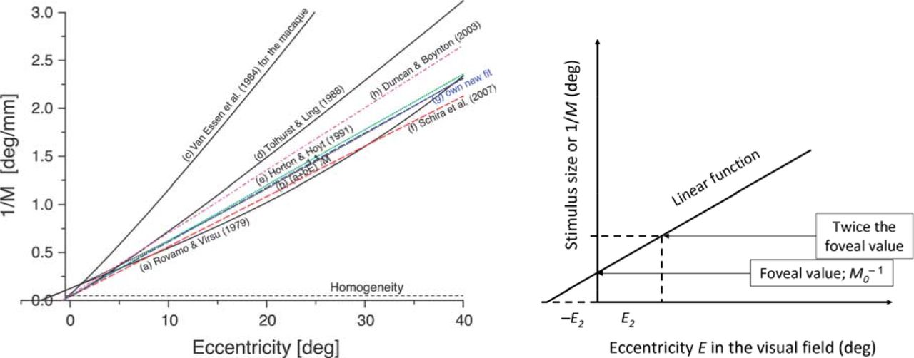
A. The inverse of the cortical magnification factor, or – equivalently – the size of a patch in the visual field that projects onto a patch of constant size in the cortex, as a function of eccentricity in the visual field (Fig. 9 in Strasburger et al., 2001, reproduced for illustrating the text). All functions show a mostly linear behavior. Their slope is quite similar, with the exception of Van Essen et al.’s (1984) data for the macaque; other data show similar slopes between human and monkey (e.g. Oehler, 1985). B. An illustration of the E2 concept.
The empirical data all fit the linear concept quite well, but some slight deviations are apparent in the considered range of about 40° eccentricity. These are asides here but should be mentioned. The linear equation for the eccentricity function was often “tweaked” a little to accommodate for these deviations: Rovamo, Virsu, & Näsänen (1978) added a small 3rd-order term, Van Essen et al. (1984) and Tolhurst & Ling (1988) increased the exponent of the linear term slightly, from 1 to 1.1. Virsu & Hari (1996) took different approach and used a sine function, based on geometrical considerations, from which only a part of the sine’s period was used (one-eighth) though so that the function is still close to linear in that range. The latter function is interesting because it is the only one that – because it is bounded – can be extended to larger eccentricities, 90° and beyond (note that the visual field extends beyond 90°).
Elliptical field
Another deviation from simple uniform linearity is the fact that the visual field is not isotropic: Performance declines differently between radii (this is used by Greenwood, Danter, & Finnie, 2017 to disentangle retinal from cortical distance). Iso-performance lines for the binocular field are approximately elliptical rather than circular outside the very center (e.g. Wertheim, 1894, Harvey & Pöppel, 1972; Pöppel & Harvey, 1973, see their Fig. 6). At the transition from the isotropic to the anisotropic field (in the plateau region of Pöppel & Harvey, 1973), the scaling function (Figure 1A) thus not only has different slopes along the different meridians but also necessarily deviates from linearity. Correspondingly, early visual areas are found to be anisotropic (e.g. Horton & Hoyt, 1991). The effect of anisotropy on the cortical magnification factor is quantitatively treated by Schira et al. (2007) (not covering the plateau, though); their M0 estimate is the geometric mean of the isopolar and isoeccentric M estimates. In the equations presented below, the anisotropy can be accommodated by letting the parameters depend on the radius in question. A closed analytical description is presented by Schira et al. (2010).
The E2 concept
For a quick comparison of eccentricity functions for psychophysical tasks, Levi et al. (1984, p. 794) introduced E2 – a value which denotes the eccentricity at which the foveal threshold for the corresponding task doubles (Figure 1B illustrates this). More generally, E2 is the eccentricity increment at which the threshold increases by the foveal value. As a graphic aide, note that this value is also the distance of where the linear function crosses the eccentricity axis from the origin (i.e., E2 is the negative abscissa intercept in Figure 1B).
Eq. (1) below states the equation using E2. The function’s slope is given by the fraction  , so when these functions are normalized to the foveal value their slope is
  . E2 thus captures an important property of the functions in a single number. A summary of values reported over the years is given in Strasburger et al. (2011, Tables 4–6). These reported E2 values vary widely between different visual functions. They also vary considerably for functions that seem directly comparable to each other (Vernier: 0.62–0.8; M−1 estimate: 0.77–0.82; Landolt-C: 1.0–2.6; letter acuity: 2.3–3.3; gratings: 2.5–3.0). Note also the limitations of E2: since the empirical functions are never fully linear for example, the characterization by E2, by its definition, works best at small eccentricities.
The two centers
There is an important difference in difficulty between assessing the fovea’s center and the cortical retinotopic center. Whereas for psychophysical tests the measurement of the foveal value is particularly simple and reliable, the opposite appears to be the case for the anatomical foveal counterpart,  . The latter is considered the most difficult to determine and is mostly extrapolated from peripheral values. The consequences of this include a different perspective on research on the map between the two fields. We will come back to that below.
Using the E2 parameter, the inverse-linear scaling function can be concisely and elegantly stated as

M−1 in the equation, measured in °/mm, is defined as the size of a stimulus in degrees visual angle at a given point in the visual field that projects onto 1 mm cortical V1 diameter.  is that value in the fovea center. The left hand ratio in the equation,
  , is the ratio by which a peripherally seen stimulus needs to be size-scaled to occupy cortical space equal to a foveal stimulus. So the equation can equally well be written as
 where S is scaled size and S0 is the size at the fovea’s center. From eq. (1),
  can be considered the size-scaling unit in the visual field, and E2 the locational scaling unit (i.e. the unit in which scaled eccentricity is measured).
2. Goal of the Paper
Three goals are pursued in this paper. Firstly, relationships are derived that translate the nomenclature of psychophysics to that in cortical physiology. The approaches are closely linked, and results on the mapping functions can be translated back and forth. The key equations for the cortical location function will be eq. (10) and eq. (16) plus (17). The usefulness of these equations is shown in a subsequent section.
Secondly, it is explored how the cortical function looks like in the popular simplified case with omitted constant term (Figure 2). Read this if you believe one can get away with it, and explore the absurdities that ensue. It is argued there that this might have been a good solution at the time but not now when we have detailed knowledge of the cortical mapping close to the retinotopic center: The linear M-scaling function shown in Figure 1 is accurate down to very low eccentricities whereas that is not the case for the simplified location function. It makes little sense to continue working with equations that do not, and cannot, apply over the whole range.

Illustration of the cortical location function introduced by Schwartz (1980). A version with and another without a constant term (parameter b in the equation) is shown. The constant term was intended as a simplification for large eccentricities but is physically impossible for the foveal center. The graph shows E as a function of d, which is an exponential; Schwartz (1980) discussed it mainly the inverse function, i.e. for cortical distance d as a function of eccentricity E, which is logarithmic.
Conversely, to show the usefulness of the derived improved equations, a section explores practical examples for the cortical mapping function, with data from the literature. The graphs look like those in Figure 2 but have realistic parameter values. Comprehensive and concise mathematical descriptions have been derived before (Schira, Tyler, et al., 2010); the purpose here is to do so in an easily applicable way and with the nomenclature from psychophysics, (i.e., using E2).
Thirdly, and finally, these concepts are applied to the cortical map for crowding. Crowding, i.e. the impaired recognition of a pattern in the presence of neighbors, is probably the prominent characteristic of peripheral vision. Interestingly, unlike the perceptual tasks discussed in the preceding, where critical size scales with eccentricity (e.g. acuity or contrast sensitivity), crowding is mostly independent of target size. Instead, the critical distance between target and flankers scales with eccentricity. This characteristic has become to be known as Bouma’s Law, following Bouma’s (1970) seminal paper where it was first stated. Now, Bouma’s Law follows the same linear eccentricity law as stated in eq. (1) or eq. (2) and depicted in Figure 1. This time, however, it refers to distance between patterns instead of size of patterns. Consequently, the E2 concept can be applied in the same way. The cortical location function that we derive in the first part can then be used to predict the cortical distances that correspond to the flanker distances in Bouma’s Law.
Topically, this cortical critical crowding distance has been proposed being a constant (Motter & Simoni, 2007; Pelli, 2008; Mareschal, Morgan, & Solomon, 2010). We will show here that this assumption is most likely incorrect. It rests on the same confusion of linearity and proportionality that gives rise to the poppycock1 of a cortical location function that misses the retinotopic center (discussed in Section 3.3). In any case, the result derived for critical cortical crowding distance (CCCD) will be that it increases within the fovea and reaches an asymptote further out (thus being consistent with constancy at sufficient eccentricity).
In the derivations given in the following, care was taken to phrase the steps so as to be easy to follow. Yet a legitimate way of using the paper would also be to take the final results as take-home message. That would be eq. (10) or (13) for the cortical mapping of the visual field (i.e. the cortical location function), eq. (8) for the new parameter d2, eq. (17) for M0, and eq. (32)–(34) for the mapping of Bouma’s rule onto the cortex.
3. Cortical location
3.1 Cortical location specified relative to the retinotopic center
In psychophysical experiments, the ratio  in eq. (1) is readily estimated as the size of a stimulus relative to a foveal counterpart for achieving equal perceptual performance in a low-level task. However, in physiological experiments M is difficult to assess directly (even though it is a physiological concept). Instead, it is typically derived – indirectly – from the cortical-location function d = d(E). That function links a cortical distance d, in a retinotopic area, to the corresponding distance in the visual field that it represents (see the x-axis in Figure 2). More specifically, d is the distance (in mm) on the cortical surface between the representation of a visual-field point at eccentricity E, and the representation of the fovea center. Under the assumption of linearity of the cortical magnification function, M−1(E), this function is logarithmic (and its inverse E = E(d) is exponential as in Figure 2), as has been shown previously by Schwartz (1980). And, since E2 allows a simple formulation of cortical magnification function in psychophysics, as e.g. in eq. 1, it will be useful to state the equation d = d(E) with those notations. This is the goal of the paper. The location function allows a concise quantitative characterization of the early retinotopic maps. (Symbols used in the paper are summarized in Table 1 for convenience.)
Summary of symbols used in the paper
To derive the cortical location function notice that, locally, the cortical distance of the respective representations d(E) and d(E+ΔE) of two nearby points along a radius at eccentricities E and E+ΔE is given by M(E)∙ΔE. (This follows from M’s definition and that M refers to 1°). The cortical magnification factor M is thus the first derivative of d(E),

Conversely, the location d on the cortical surface is the integral over M (starting at the fovea center)

If we insert eq. (1) (i.e. the equation favored in psychophysics) into eq. (4), we have
 where ln denotes the natural logarithm (cf. Schwartz, 1980).
The inverse function, E(d), which derived by inverting eq. (5), is

It states how the eccentricity E in the visual field depends on the distance d of the corresponding location in a retinotopic area from the point representing the fovea center. With slight variations (discussed below) it is the formulation often referenced in fMRI papers on the cortical mapping. Note that by its nature it is only meaningful for positive values of cortical distance d.
We can simplify that function further by introducing an analogue to E2 in the cortex. Like any point in the visual field, E2 (on the meridian in question) has a representation and we denote the distance d of its location from the retinotopic center as d2. Thus, d2 represents E2. At that location, eq. (6) implies

We solve this for the product M0E2,

Inserting that in eq. (6) gives

Eq. (9) is the most concise way of stating the cortical mapping function. However, since the exponential to the base e is often more convenient, it can be restated as
 (here, ln again denotes the natural logarithm).
This equation (eq. 10) is particularly nice and simple provided that d2, the cortical equivalent of E2, is known. That value, d2, could thus play a key role in characterizing the cortical map, similar to the role of E2 in visual psychophysics (cf. Table 4 – Table 6 in Strasburger et al., 2011). Estimates for d2 derived from literature data are summarized in Section 3.4 below, as an aid for concisely formulating the cortical location function.
3.2 Cortical location specified relative to a reference location
Implicit in the definition of d or d2 is the knowledge about the location of the fovea center’s cortical representation, i.e. of the retinotopic center.1 However, that locus appears to be hard to determine. Instead of the center it has thus become customary to use some fixed eccentricity Eref as a reference. Engel et al. (1997, Fig. 9), for example, use Eref = 10°. Larsson & Heeger (2006, Fig. 5) use Eref = 3°.
To restate eq. (6) accordingly, i.e. with a reference eccentricity different from Eref = 0, we first apply eq. (10) to the reference:
 where dref denotes the value of d at the chosen reference eccentricity, e.g. at 3° or 10°.
Solving that equation for d2 and plugging the result into eq. (9) or (10), we arrive at

Expressed to the base e, we then have

One could also derive eq. (13) directly from eq. (6). Note that if, in that equation, we take E2 as the reference eccentricity, it reduces to eq. (10). So E2 can be considered as a special case of a reference. Note further that, unlike the equations often used in the fMRI retinotopy literature, the equations are well defined in the fovea center: for d = 0, eccentricity E is zero, as it should be.
What reference to choose is up to the experimenter. However, the fovea center itself cannot be used as a reference eccentricity – the equation is undefined for dref = 0 since the exponent is then infinite. The desired independence of knowing the retinotopic center’s location has also not been achieved: That knowledge is still needed, since d, and dref, in these equations are defined as the respective distances from that point.
Equations (12) and (13) have the ratio d/dref in the exponent. It is a proportionality factor for d from the zero point. From the intercept theorem we know that this factor cannot be re-expressed by any other expression that leaves the zero point undefined. True independence from knowing the retinotopic center (though desirable) thus cannot be achieved.
We can nevertheless shift the coordinate system such that locations are specified relative to the reference location, dref. For this, we define a new variable  as the cortical distance (in mm) from the reference dref instead of from the retinotopic center (see Figure 3 for an illustration for the shift and the involved parameters), where dref is the location corresponding to some eccentricity, Eref. By definition, then,


Illustration of the cortical distance measures used in equations (6) – (23), and of parameter b in eq. (18).
d – cortical distance of some location from the retinotopic center, in mm;
dref – distance (from the center) of the reference that corresponds to Eref;
d1° – distance of the location that corresponds to E = 1°;
 – distance of location d from the reference dref.
In the shifted system – i.e., with  instead of d as the independent variable – eq. (6) for example becomes

However, unlike eq. (6), this equation is not yet useful because – as will be shown in eq. (17) below – the three parameters in it are not all free: M0, E2, and dref cannot be chosen independently.
Similarly, eq. (13) in the shifted system becomes

That equation has the advantage over eq. (15) of having only two free parameters, E2 and dref (Eref is not truly free since it is empirically linked to dref). The foveal magnification factor M0 has dropped from the equation. Indeed, by comparing eq. (13) to eq. (6) (or by comparing eq. (15) to (16)), M0 can be calculated from dref and E2 as
 where β is defined as in the previous equation. With an approximate location of the retinotopic center (needed for calculating dref) and an estimate of E2, that latter equation leads to an estimate of the foveal magnification factor, M0 (see Section 3.4 for examples).
Equations (16) and (17) are crucial to determining the retinotopic map in early areas. They should work well for areas V1 to V4 as discussed below. The connection between the psychophysical and physiological/fMRI approaches in these equations allows cross-validating the empirically found parameters and thus leads to more reliable results. Duncan & Boynton (2003), for example, review the linear law and also determine the cortical location function empirically but do not draw the connection. Their’s and others’ approaches are discussed as practical examples in the section after next (Section 3.4).
3.3 Independence from the retinotopic center with the simplified function
A seemingly more practical approach is taken in several papers in the fMRI retinotopy literature. Data are expressed as in the equations above as  (i.e. as a function of cortical distance from some reference location) yet unlike eq. (5) or (6) and those that follow from it, are derived from the simplified exponential/logarithmic law proposed by Schwartz (1980). As said above the simplified version omits the constant term (“–1” in eq. 6 to eq. 16) and works well for sufficiently large eccentricities. Thus, the equation
 is fit to the empirical data, with free parameters a and b. The distance variable is then
  as before, i.e., the cortical distance in mm from a reference that represents some eccentricity Eref in the visual field. For such a reference, Engel et al. (1997, Fig. 9) for example use Eref = 10°, and for that condition the reported equation is
  . Larsson & Heeger (2006, Fig. 5) use Eref = 3°, and for area V1 in that figure give the function
  .
.
We can attach meaning to the parameters a and b in eq. (18) by looking at two special points,  and
and  : At the point
  , eccentricity E equals 1° visual angle (from the equation), so we can call that value
  and b thus is

The value of  is negative; it is around −36.5 mm for Eref = 10° and is the distance of the 1° line from the reference eccentricity’s representation (where
  ). At
). At  , on the other hand, E = Eref by definition, and from eq. (18) we have

Now that we have parameters a and b we can insert those in the above equation and rearrange terms, by which we get
 or, expressed more conveniently to the base e,

This is now the simplified cortical location function (the simplified analog to eq. 16), with parameters spelt out. One can easily check that the equation holds true at the two defining points, i.e. at 1° and at the reference eccentricity. Note also that, as intended, knowing the retinotopic center’s location in the cortex is not required since  is defined relative to a non-zero reference. Obviously, however, the equation fails increasingly with smaller eccentricities, for the simple reason that E cannot become zero. In other words, the fovea’s center is never reached even (paradoxically) when we are at the retinotopic center. Equation (18), or (21), (22) are thus better avoided.
To observe what absurdities happen towards eccentricities closer to the fovea center, let us express the equation relative to the absolute center. From eq. (14) and
 it follows
 where d as before is the distance from the retinotopic center. Naturally, by its definition, the equation behaves well at the two defining points (resulting in the values Eref, and 1°, respectively). However, in between these two points the function has the wrong curvature (see Fig. 4 in the next section) and at the fovea center (i.e. at d = 0), the predicted eccentricity – instead of zero – takes on some obscure non-zero value E0 given by

As seen in the equation the value depends on the chosen reference eccentricity, its representation, and the cortical representation of 1° eccentricity, all of which it shouldn’t. So the seeming simplicity of eq. (18) leads astray in the fovea, which, after all, is of paramount importance for vision. The next section illustrates the differences between the two sets of equations with data from the literature.
3.4 Practical use of the equations: examples
3.4.1 The approach of Larsson & Heeger (2006)
Now that we have derived two sets of equations for the location function (i.e. with and without a constant term, in Section 3.1 and 3.3, respectively) let us illustrate the difference with data on the cortical map for V1 from Larsson & Heeger (2006, Fig. 5). As a reminder, this is about eq. (16) on the one hand – in essence  , derived from eq. (6) – and eq. (24) on the other hand (
 , derived from eq. (18).
For the reasons explained above the retinotopic center is left undefined by Larsson & Heeger (2006) and a reference eccentricity of Eref = 3° is used instead. The fitted equation in the original graph is stated as  , which corresponds to eq. (18) with constants a = 0.0577 and
  . Its graph is shown in Figure 4 as the thick black line copied from the original graph, that is continued to the left as a dotted blue line. At the value of −b, i.e. at a distance of
  mm from the 3° representation (as seen from eq. 19), the line crosses the 1° point. To the left of that point, i.e. towards the retinotopic center, the curve deviates markedly upward and so the retinotopic center (E = 0°) is never reached.

Comparison of conventional and improved functions for describing the cortical location function, (retinal eccentricity vs. corresponding cortical location). Symbols and fat black line show the retinotopic data for area V1 with dref = 3° from Larsson and Heeger (2006, Fig. 5) (symbols for 9 subjects) together with the original fit, according to eq. (18)  or (22). I.e. this is a fit without a constant term. The blue dotted line continues that fit to lower eccentricities; the fitted
  function goes to (negative) infinite cortical distance which is physically meaningless. Pink and green line: graphs of (the preferable) eq. (16), derived from integrating the inverse linear law (eq. 1), with two different parameter choices; [E2 = 0.6°, dref = 38 mm] and [E2 = 1.0°, dref = 35 mm], respectively. The retinotopic center’s magnification factor M0 can be calculated by eq. (17) as 35.4 mm/° and 25.3 mm/° for the two cases, respectively. Black and brown line:
  function with parameters derived by Duncan & Boynton (2003), M0 = 18.5 mm/° and E2 = 0.831°(black), and with dref = 15.5 mm (brown) for comparison. Note that, by definition, the curves pass through 3° at
  mm. Note also that data beyond ~10 mm were said to be biased by the authors and can be disregarded.
The pink and the green curve in Figure 4 are two examples for a fit of the equation with a constant term (i.e. for eq. 16). The pink curve uses E2 = 0.6° and dref = 38 mm, and the green curve E2 = 1.0° and dref = 35 mm. Note that smaller E2 values go together with larger dref values for a similar shape. Within the range of the data set, the two curves fit about equally well; the pink curve is slightly more curved (a smaller E2 is accompanied by more curvature). Below about 1° eccentricity, i.e. around half way between the 3° point and the retinotopic center, the two curves deviate markedly from the original fit. They fit the data there better and, in particular, they reach a retinotopic center. The pink curve (with E2 = 0.6°) reaches the center at 38 mm from the 3° point, and the green curve at 35 mm.
The central cortical magnification factor M0 for the two curves can be derived from eq. (17), giving a value of 35.4 mm/° and 25.3 mm/°, respectively. These two estimates differ substantially – by a factor of 1.4 – even though there is only a 3-mm difference of the assumed location of the retinotopic center. This illustrates the large effect of the estimate for the center’s location on the foveal magnification factor, M0. It also illustrates the importance of a good estimate for that location.
There is a graphic interpretation of the foveal magnification factor M0 in these graphs. From eq. (6) one can derive that  is equal to the function’s slope at the retinotopic center. Thus, if the function starts more steeply (as does the green curve compared to the pink one),
  is higher and thus M0 smaller.
The figure also shows two additional curves (black and brown), depicting data from Duncan & Boynton (2003), as discussed below. To better display the various curves’ shapes, they are shown again in Figure 5 but without the data symbols. Figure 5 also includes an additional graph, depicting the exponential function  reported by Engel et al. (1997). In it,
  is again the cortical distance in millimeters but this time from the 10° representation. E, as before, is the visual field eccentricity in degrees. For comparison with the other curves, the curve is shifted (by 19.1 mm) on the abscissa to show the distance from the 3° point. The curve runs closely with that of Larsson & Heeger (2006) and shares its difficulties.

Same as Figure 4 but without the data symbols, for better visibility of the curves. The additional dash-dotted curve next to that of Larsson & Heeger’s depicts the earlier equation by Engel et al. (1997).
3.4.2 The approach of Duncan & Boynton (2003)
Figure 4 and Figure 5 show a further  function that is based on the results of Duncan & Boynton (2003). That function obviously differs quite a bit from the others in the figure and it is thus worthwhile studying how Duncan & Boynton derived these values. The paper takes a somewhat different approach for estimating the retinotopic mapping parameters for V1 than the one discussed before.
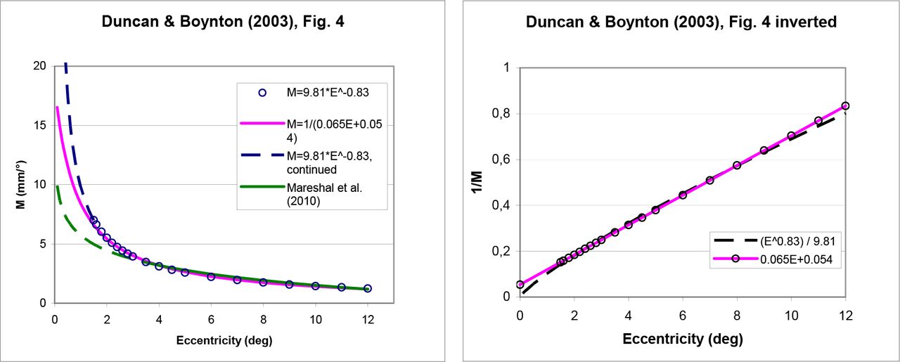
As a first step in Duncan & Boynton’s paper, the locations of the lines of equal eccentricity are estimated for five eccentricities (1.5°, 3°, 6°, 9°, 12°) in the central visual field, using the equation w = k * log (z + a). The function looks similar to the ones discussed above except that z is now a complex variable that mimics the visual field in the complex plane. On the horizontal half-meridian, though, that is equivalent to eq. (6) in the present paper, i.e., to an E(d) function with a constant term (parameter a) and with the retinotopic center as the reference. At these locations the authors then estimate the size of the projection of several 1°-patches of visual space (see their Fig. 3; this is where they differ in their methodology). By definition, these sizes are the cortical magnification factors Mi at the corresponding locations. Numerically, these sizes are then plotted vs. eccentricity in their Fig. 4. Note, however, that this is not readily apparent from the paper, since both the graph and the accompanying figure caption state something different. In particular the y-axis is reported incorrectly (as is evident from the accompanying text). For clarity, therefore, Figure 6 here plots these data with a corrected label and on a linear y-axis.

(A) Duncan & Boynton’s (2003) Fig. 4, drawn on a linear y-axis and with a corrected y-axis label (M in mm/°). Note that the equation proposed earlier in the paper (p. 662), M = 9.81*E−0.83, predicts an infinite foveal magnification factor (blue curve). In contrast, the inverse-linear fit M−1 = 0.065 E + 0.054 proposed later in the paper (p. 666) fits the data equally well in the measured range of 1.5° to 12° but predicts a reasonable foveal magnification factor of 18.5 mm/°. The E2 value for the latter equation is E2 = 0.83. The additional green curve shows an equation by Mareschal et al. (2010) (see next section). (B) The inverse of the same functions. Note the slight but important difference at 0° eccentricity, where the linear function is non-zero and its inverse is thus well-defined.
The authors next fit a power function to those data, given as M = 9.81*E−0.83 for the cortical magnification factor (see Figure 6). There is a little more confusion, however, because it is said that from such power functions the foveal value can be derived by extrapolating the fit to the fovea (p. 666). That cannot be the case, however, since – by the definition of a power function (including those used in the paper, both for the psychophysical and for the cortical data) – there is no constant term. The function therefore goes to infinity towards the fovea center, as shown in Figure 6 (dashed line). Furthermore, E2, which is said to be derived in this way in the paper, cannot be derived from a nonlinear function (because the E2 concept requires a linear or inverse-linear function). The puzzle is resolved, however, with a reanalysis of Duncan & Boynton’s Fig. 4: it reveals how the foveal value and the connected parameter E2 were, in fact, derived – an inverse-linear function fits the data equally well in the measured range of 1.5° – 12° eccentricity (Figure 6, continuous line). From that function, the foveal value and E2 are readily derived. Indeed, they correspond to the values given in the paper.
Duncan & Boynton (2003) do not specify the distance of the isoeccentricity lines from the retinotopic center. We can derive it from eq. (17) though because M0 and E2 are fixed:

With their parameters (M0 = 18.5 mm/° and E2 = 0.83), the scaling factor β comes out as β= 1.03 (from eq. 16). From that, dref = d1.5° = 15.87 mm. As a further check we can also derive a direct estimate of dref from their Fig. 3. For subject ROD, for example, the 1.5° line is at a distance of d1.5° = 15.45 mm on the horizontal meridian. That value is only very slightly smaller than the one derived above; so, for illustration, Figure 4 and Figure 5 also contain a graph for that value. Conversely, with dref given, M0 can be derived from eq. (17) (or eq. 26), which gives a slightly smaller value of M0 = 18.0 mm/°. The two curves are hardly distinguishable; thus, as previously stated, dref and M0 interact, with different value-pairs resulting in similarly good fits.
In summary, the parameters in Duncan & Boynton’s (2003) paper: M0 = 18.5 mm/° and E2 = 0.83, are supported by direct estimates of the size of 1°-projections. They are taken at locations estimated from a set of mapping templates which themselves are derived from a realistic distance-vs.-eccentricity equation. The paper provides another good example how the linear concept for the magnification function can be brought together with the exponential (or logarithmic) location function. The estimate of M0 comes out considerably lower, however, than in more recent papers (e.g. Schira et al., 2009; see Figure 7 below). Possibly the direct estimation of M at small eccentricities is less reliable than the approach taken in those papers.
3.4.3 Mareschal, Morgan & Solomon (2010)
Figure 6 shows an additional curve from a paper by Mareschal et al. (2010) on cortical distance, who base their cortical location function partly on the equation of Duncan & Boynton (2003). Mareschal et al. (2010) state their location function as

The upper part of the equation is that of Duncan & Boynton (pink curve), used below 4°, the green continuous line shows Mareschal’s log equation above 4°, and the dashed line shows how the log function would continue for values below 4°. Obviously, the latter is off, and undefined at zero eccentricity, which is why Mareschal et al. then switch to the inverse-linear function (i.e. the mentioned pink curve). The problem at low eccentricity is apparent in Fig. 9 in their paper where the x-axis stops at ½ deg, so the anomaly is not fully seen. For their analysis it is not relevant since only two eccentricities, 4° and 10°, were tested. The example is added here to illustrate that our new equations would have allowed for a single equation with no need for case distinctions.
3.4.4 Toward the retinotopic center
As discussed above, predictions of the retinotopic center depend critically on its precise location and thus require data at small eccentricities. Schira, Tyler and coworkers have addressed that problem in a series of papers (Schira et al., 2007; Schira, Tyler, Breakspear, & Spehar, 2009; Schira et al., 2010) and provide detailed maps of the centers of the early visual areas, down to 0.075° eccentricity. They also develop parametric, closed analytical equations for the 2D maps. When considered for the radial direction only, the equations correspond to those discussed above (eq. 1 and eq. 16/17).
Figure 7 shows magnification factors from Schira et al., 2009, Fig. 7A, with figure part B showing their V1 data (red curve), redrawn on double-linear coordinates. As can be seen, the curve run close to an hyperbola. Its inverse is shown in Figure 7C, which displays the familiar, close-to-linear behavior over a wide range with a positive y-axis intercept that corresponds to the value at the fovea center,  . From the regression line, M0 and E2 are readily obtained and are E2 = 0.21° and M0 = 47.6 mm, respectively. Note that a rather large value of M0 is obtained compared to previous reports. However, as can also be seen from the graph, if one disregards the most peripheral point, the centrally located values predict a somewhat shallower slope of the linear function with a thus slightly larger E2 and smaller M0 value: E2 = 0.33° and M0 = 34.8 mm. The latter values might be the more accurate predictors for V1’s very center.

Cortical magnification factor from Schira, Tyler, Breakspear & Spehar (2009, Fig. 7A). (A) Original graph. (B) V1 data for M from Schira et al.’s graph but drawn on double-linear coordinates. (C) Resulting inverse factor, again on linear coordinates. The regression line, M−1 = 0.0977E + 0.021, fits the whole set –1 and predicts E2 = 0.21° and M0 = 47.6 mm. The regression equation M−1 = 0.0867E + 0.0287 is a fit to the first four points and might be a better predictor for the retinotopic center, giving E2 = 0.33° and M0 = 34.8 mm.
In summary, the derived equations provide a direct link between the nomenclature used in psychophysics and that in neurophysiology on retinotopy. They were applied to data for V1 (Fig. 2) but will work equally well for higher early visual areas, including V2, V3, and V4 (cf. Larsson & Heeger, 2006, Fig. 5; Schira et al., 2009, Fig. 7). M0 is expected to be slightly different for the other areas (Schira et al., 2009, Fig. 7)) and so might be the other parameters.
3.4.5 d2 – a parameter to describe the cortical map
As shown in Section 3.1 (eq. 9 or 10), a newly defined parameter d2 can be used to describe the cortical location function very concisely. Parameter d2 is the cortical representation of Levi’s E2, i.e. the distance (in mm) of the eccentricity (E2) where the foveal value doubles from the retinotopic center. Eq. (8) can serve as a means to obtain an estimate for d2. Essentially, it is the product of M0 and E2. Table 2 gives a summary of d2 estimates thus derived.
d2 values from a reanalysis of data in several studies, by eq. (8): d2 = M0 E2 ln(2) *M0 was not estimated in that paper; the mean of the preceding M0 values is used for the calculation instead.
4. Crowding and Bouma’s Law in the cortex
In the final section the equations will be applied to an important property of cortical organization: visual crowding. Whereas in the preceding, cortical location was the target of interest, in this section we are concerned with cortical distances.
As said in the introduction, for MAR-like functions like acuity, a general property of peripheral vision is that critical size scales with eccentricity so that deficits can mostly be compensated for by M-scaling. For crowding, in contrast, target size plays little role (Strasburger, Harvey, & Rentschler, 1991; Pelli, Palomares, & Majaj, 2004). Instead, the critical distance between target and flankers scales with eccentricity, though at a different rate than MAR. This characteristic of crowding has been termed Bouma’s Law since Strasburger et al. (1991) and Pelli et al. (2004) drew attention to the seminal paper where it was first stated (Bouma, 1970). The corresponding distances in the primary cortical map are thus governed by differences of the location function derived here in the first section. Crowding is, in a sense, thus a spatial derivative of location and a spatial-vision task that might reflect the difference between detection and recognition processes (Strasburger & Rentschler, 1996; Heinrich & Bach, 2013). Pattern recognition, as is now increasingly recognized, is largely unrelated to visual acuity (or thus to cortical magnification) and is, rather, governed by the crowding phenomenon (Strasburger et al., 1991; Pelli et al., 2004; Pelli et al., 2007; Pelli & Tillman, 2008; Strasburger & Wade, 2015a). For understanding crowding it is paramount to look at its cortical basis, since we know since Flom, Weymouth, & Kahnemann (1963) that crowding is of cortical origin, as also emphasized by Pelli (2008).
Now with respect to this cortical distance, it has been proposed more recently that it is likely a constant (Motter & Simoni, 2007; Pelli, 2008; Mareschal et al., 2010). Elegant as it seems, however, it will be shown here that this assumption is most likely false. If stated as a general rule, it rests on the same confusion of linearity and proportionality – i. e. the omission of the constant term – that gave rise to those dubious cortical location functions that miss the retinotopic center (discussed in Section 3.3). Based on the properties of the cortical location function derived in Section 3., it will turn out that the critical cortical crowding distance (CCCD) increases within the fovea (where reading mostly takes place!) and reaches an asymptote beyond perhaps 5° eccentricity, consistent with a constancy at sufficient eccentricity. Consistent with this, Pelli (2008) warns against extrapolating the constancy toward the retinotopic center.
Let us delve into the equations. Bouma (1970) stated in a short Nature paper what is now known as Bouma’s law for crowding:
 where δspace is the free space between the patterns at the critical distance1 and b is a proportionality factor. Bouma (1970) proposed an approximate value of b = 0.5 = 50%, which is now widely cited, but he also mentioned that other proportionality factors might work equally well. Indeed, Pelli et al. (2004) have shown that b can take quite different values, depending on the exact visual task, but that linearity holds in each case. In fairness to Bouma the law is thus best stated as saying that free space for critical spacing is proportional to eccentricity, the proportionality factor taking some value around 50% depending on the task.
Today it has become customary to state flanker distance not as free space but as measured from the respective centers of the target and a flanker. To restate Bouma’s rule for the center-to-center distance between the patterns, δ, let the target pattern have the size S in the radial direction (i.e., width in the horizontal), so that δ = S + δspace. Eq. (27) then becomes

This equation is no longer proportionality yet is still linear in E. Analogously to Levi’s E2 we thus introduce a parameter  where the foveal value of critical distance doubles. Denoting the foveal value of critical distance by δ0, we get from eq. (28):

Obviously, that equation is analogous to eq. (1) and (2) that we started out with; it describes how critical distance in crowding – like acuity and many other spatial visual performance measures – is linearly dependent on, but is not proportional to, eccentricity in the visual field.
With the equations derived in the preceding sections we can derive the critical crowding distance in the cortical map, i.e. the cortical representation of critical distance in the visual field. Let us denote that distance by κ (kappa). By definition, it is the difference between the map locations for the target and a flanker at the critical distance in the crowding task: κ = df−dt. The two locations are in turn obtained from the mapping function, which is given by inverting eq. (6) above:

As before, d is the distance of the location in the cortical map from the retinotopic center. So, critical distance κ for crowding in the retinotopic map is the difference of the two d values,
 (by eq. 30 and 29), where Et and Ef are the eccentricities for target and flanker, respectively. After simplifying and setting target eccentricity E1 = E for generality, this becomes

Note that we formulated that equation in previous publications – but incorrectly as I am sorry to say (Strasburger & Malania, 2013, eq. 13, and Strasburger et al., 2011, eq. 28): a factor was missing there.
Let us explore this function a little; its graph is shown in Figure 8. In the retinotopic center, equation (32) predicts a critical distance κ0 in the cortical map of

With increasing eccentricity, κ departs from that foveal value and increases (or possibly decreases), depending on the ratio  . Numerator and denominator are the E2 values for the location function and crowding function, respectively (eq. 1 vs. eq. 29). They depend on their function’s respective slope and are generally different, so that their ratio is not unity. With sufficiently large eccentricity, the equation converges to

The latter expression is identical to that for the foveal value in eq. (33) except that E2 is now replaced by the corresponding value  for crowding.

Graph of eq. (32) with realistic values for M0, E2,  , and δ0. The value of E2 for M−1 was chosen as E2 = 0.8° from Dow, Snyder, Vautin, & Bauer, 1981 (as cited in Levi, Klein, & Aitsebaomo, 1985 or Strasburger et al., 2011, Table 4). M0 = 29.1 mm was chosen to give a good fit with this E2 in Fig. 2. Foveal critical distance was set to δ0 = 0.1° from Siderov, Waugh, & Bedell, 2013, 2014. An
  would obtain with this δ0 and the value of δ4° = 1.2° in Strasburger et al., 1991; it also serves as an example for being a clearly different value than E2 for the cortical magnification factor, to see the influence of the
  ratio on the graph. Cortical critical distance κ starts from the value given in eq. (33) (around 2 mm) and converges to the value in eq. (34).
Importantly, note that kappa varies substantially around the center, by around two-fold between the center and 5° eccentricity with realistic values of E2 and  . This is at odds with the conjecture that the cortical critical crowding distance should be a constant (Motter & Simoni, 2007; Pelli, 2008; Mareschal et al., 2010). Indeed, Pelli (2008) presented a mathematical derivation, very similar to the one presented here – based on Bouma’s law and Schwartz’ (1980) logarithmic mapping function – that comes to the conclusion of constancy. The discrepancy arises from different assumptions. Pelli used Bouma’s law as proportionality, i.e., in its simplified form stated in eq. (27) (its graph passing through the origin). The simplification was done on the grounds that outside the center the error is small and plays little role, and the paper warns that additional provisions must be made at small eccentricities. Schwartz’ mapping function was consequently also used in its simplified form (also leaving out the constant term), for the same reason. With these simplifications the critical distance in the cortex indeed turns out as simply a constant.
As should be expected, at sufficiently high eccentricities κ is close to constant in the derivations given above (Figure 8). These equations (eq. 32–34) can thus be seen as a generalization of Pelli’s result that now also covers the (obviously important) case of central vision.
That said, an interesting (though unlikely) special case of eq. (32) is the one in which E2 and  are equal. κ is then a constant, as Pelli (2008) predicted. Its value in that case would be simply given by

On a different note, equations (32)–(35) have M0 as a scaling factor and, as said before, M0 is notoriously difficult to determine empirically. However, M0 can be replaced, as shown above. From eq. (17) we know that
 which, by the definition of β, takes a particularly simple form when d2 (the cortical equivalent of E2) is chosen as the reference:

We can then rewrite the equation for the cortical crowding critical distance (eq. 32) as

Similarly, the two special cases eq. (33) and (34) become
 and
and

Values for d2 derived from the literature by eq. (37) that could be plugged into eq. (39) and (40) were provided in Table 2 above. These two equations, for the retinotopic center and eccentricities above around 5°, respectively, could lend themselves for determining critical crowding distance in the cortex.
In summary for cortical crowding distance, the linear eccentricity laws in psychophysics for cortical magnification and for critical crowding distance – both well established – together with Schwartz’ equally well-established logarithmic mapping rule, predict a highly systematic behavior of crowding’s critical distance in the cortical map. Given the very similar mappings in areas V2, V3, V4 (Larsson & Heeger, 2006; Schira et al., 2009), that relationship should be expected to hold in those areas as well(see Figure 8 for a graph). Since the cortical location function is well established and the equations for crowding follow mathematically, they should work well if fed with suitable E2 values. Thus, direct confirmations of their behavior would cross-validate mapping models and might shed light on the mechanisms underlying crowding.
5. Outlook
Where does this leave us? The early cortical visual areas appear very regularly organized. And, as apparent from the fMRI literature reviewed above and earlier literature, the spatial maps of early visual areas appear to be pretty similar. Yet variations of visual performance across the visual field differ widely between visual tasks, as highlighted e.g. by their respective E2 values. The puzzle of how different spatial scalings in psychophysics emerge on a uniform cortical architecture is still unresolved. Certainly, though, there can be only one valid location function on any radius; so the equivalence between psychophysical E2 and the cortical location function in the preceding equations can only hold for a single E2. That value is probably the one pertaining to certain low-level tasks, and likely those tasks that are somehow connected to stimulus size. In contrast,  for critical crowding distance is an example for a psychophysical descriptor that is not linked to stimulus size (Strasburger et al., 1991; Pelli et al., 2004); it rather reflects location differences, as discussed in Section 4. The underlying cortical architecture that brings about different psychophysical E2s (like
  ) could be neural wiring differences, within or between early visual areas.
To go further, one of the basic messages of the cortical-magnification literature is the realization that M-scaling equalizes some, but not all, performance variations across the visual field (Virsu et al., 1987; Strasburger et al., 2011, Section 3.5). In parameter space these other variables would be said to be orthogonal to target size. For pattern recognition, pattern contrast is such a variable (Strasburger, Rentschler, & Harvey, 1994; Strasburger & Rentschler, 1996). Temporal resolution is another example (Poggel, Calmanti, Treutwein, & Strasburger, 2012). Again, differing patterns of connectivity between retinal cell types, visual areas, and along different processing streams might underlie these performance differences. The aim of the present paper is just to point out that a common spatial location function underlies the early cortical architecture that can be described by a unified equation which includes the fovea and the retinotopic center, and has parameters that are common in psychophysics and physiology.
Acknowledgements
I thank Barry Lee for critical comments on the manuscript and meticulous language corrections, Zhaoping Li and Josh Solomon for critical reading, and Zhaoping Li for a thorough check of the mathematical derivations.
Footnotes
↵1 “when we divide [a string of digits] so as to constitute several objects less compounded, we can more easily estimate the number of figures” (Jurin, 1738, p. 150). Jurin reports more examples that would count as qualitative differences; see Strasburger & Wade (2015a).
↵1 “If the threshold as a function of eccentricity were a straight line passing through the origin (this does not occur and would require an infinite foveal sensitivity) the threshold would be a constant percentage of the eccentricity. It is here claimed that these curves approximate a straight line, but with a finite and positive intercept; this would lead to a decreasing percentage, falling, at first, rapidly but changing more and more slowly in the periphery. The “constant” percentage relation noted by Ogle is therefore a consequence of the straight line relationship here discussed and is secondary and less useful mathematically. Although Ogle must have observed this linear relationship, he does not seem to have developed its consequences as is here done.” (Weymouth, 1958, p. 109)
↵2 “Psychophysical procedures do not, therefore, provide a single unambiguous measure for the changes of spatial grain across the visual field.” (Westheimer, 1982, p. 157). And later: “There is a rather insistent opinion abroad that spatial visual processing has identical properties right across the visual field save for a multiplicative factor which is a function of eccentricity.” (p. 161). The term “spatial grain” in the paper’s title refers to cortical units. With respect to an explanation for vernier acuity, Westheimer writes “If the actual threshold value is a manifestation of a complex cortical processing apparatus, the distance over which it operates optimally is the more likely parameter to be found correlated with the anatomical representation of the visual field in the cortex, and this, for some reason, does not show the gross increase in grain exhibited by the threshold data.” (p. 162)”
↵1 Name of a band I played in
↵1 Eq. 8 might be taken to imply that that knowledge could be circumvented for the case of d2. But this is not the case since then M0 is required, which in turn requires knowing the retinotopic center.
↵1 “an open distance of roughly 0.5 ϕ° is required for complete isolation” (Bouma, 1970, p. 177, legend to Fig. 2)


