

Abstract
In the field of artificial intelligence, a combination of scale in data and model capacity enabled by unsupervised learning has led to major advances in representation learning and statistical generation. In biology, the anticipated growth of sequencing promises unprecedented data on natural sequence diversity. Learning the natural distribution of evolutionary protein sequence variation is a logical step toward predictive and generative modeling for biology. To this end we use unsupervised learning to train a deep contextual language model on 86 billion amino acids across 250 million sequences spanning evolutionary diversity. The resulting model maps raw sequences to representations of biological properties without labels or prior domain knowledge. The learned representation space organizes sequences at multiple levels of biological granularity from the biochemical to proteomic levels. Learning recovers information about protein structure: secondary structure and residue-residue contacts can be extracted by linear projections from learned representations. With small amounts of labeled data, the ability to identify tertiary contacts is further improved. Learning on full sequence diversity rather than individual protein families increases recoverable information about secondary structure. We show the networks generalize by adapting them to variant activity prediction from sequences only, with results that are comparable to a state-of-the-art variant predictor that uses evolutionary and structurally derived features.
1 Introduction
The size of biological sequence datasets is experiencing approximately exponential growth resulting from reductions in the cost of sequencing technology. This data, which is sampled across diverse natural sequences, provides a promising enabler for studying predictive and generative techniques for biology using artificial intelligence. We investigate scaling high-capacity neural networks to this data to extract general and transferable information about proteins from raw sequences.
The idea that biological function and structure are recorded in the statistics of protein sequences selected through evolution has a long history (Yanofsky et al., 1964; Altschuh et al., 1987; 1988). Out of the possible random perturbations to a sequence, evolution is biased toward selecting those that are consistent with fitness (Göbel et al., 1994). The unobserved variables that determine a protein’s fitness, such as structure, function, and stability, leave a record in the distribution of observed natural sequences (Göbel et al., 1994).
Unlocking the information encoded in evolutionary protein sequence variation is a longstanding problem in biology. An analogous problem in the field of artificial intelligence is natural language understanding, where the distributional hypothesis posits that a word’s semantics can be derived from the contexts in which it appears (Harris, 1954).
Recently, techniques based on self-supervision, a form of unsupervised learning in which context within the text is used to predict missing words, have been shown to materialize representations of word meaning that can generalize across problems (Collobert & Weston, 2008; Dai & Le, 2015; Peters et al., 2018; Devlin et al., 2018). The ability to learn such representations improves significantly with larger training datasets (Baevski et al., 2019; Radford et al., 2019). Can similar self-supervision techniques leveraging the growth of sequence datasets learn useful and general protein sequence representations?
In this paper, we apply self-supervision in representation learning to the problem of understanding protein sequences and explore what information can be learned. Similar to approaches used to model language, we train a neural network representation by predicting masked amino acids. For data, we use the sequences contained within the Uniparc database (The UniProt Consortium, 2007), the largest sampling of protein sequences available, spanning a wide range of evolutionary diversity. The dataset contains 250M protein sequences with 86 billion amino acids. We provide preliminary investigations into the organization of the internal representations, and look for the presence of information about biological structure and activity. We also study generalizability of the representations to new problems.
2 Background
Efficient sequence search methods have been the computational foundation for extracting biological information from sequences (Altschul et al., 1990; Altschul & Koonin, 1998; Eddy, 1998; Remmert et al., 2011). Search across large databases of evolutionary diversity assembles related sequences into multiple sequence alignments (MSAs). Within families, mutational patterns convey information about functional sites, stability, tertiary contacts, binding, and other properties (Altschuh et al., 1987; 1988; Göbel et al., 1994). Conserved sites correlate with functional and structural importance (Altschuh et al., 1987). Local biochemical and structural contexts are reflected in preferences for distinct classes of amino acids (Levitt, 1978). Covarying mutations have been associated with function, tertiary contacts, and binding (Göbel et al., 1994).
The prospect of inferring biological structure and function from evolutionary statistics has motivated development of machine learning on individual sequence families. Raw covariance, correlation, and mutual information have confounding effects from indirect couplings (Weigt et al., 2009). Maximum entropy methods disentangle direct interactions from indirect interactions by inferring parameters of a posited generating distribution for the sequence family (Weigt et al., 2009; Marks et al., 2011; Morcos et al., 2011; Jones et al., 2011; Balakrishnan et al., 2011; Ekeberg et al., 2013b). The generative picture can be extended to include latent variables parameterized by neural networks that capture higher order interactions than pairwise (Riesselman et al., 2018).
Recently, self-supervision has emerged as a core direction in artificial intelligence research. Unlike supervised learning which requires manual annotation of each datapoint, self-supervised methods use unlabeled datasets and thus can exploit far larger amounts of data, such as unlabeled sequence data. Self-supervised learning uses proxy tasks for training, such as predicting the next word in a sentence given all previous words (Bengio et al., 2003; Dai & Le, 2015; Peters et al., 2018; Radford et al., 2018; 2019) or predicting words that have been masked from their context (Devlin et al., 2018; Mikolov et al., 2013a).
Increasing the dataset size and the model capacity has shown improvements in the learned representations. In recent work, self-supervision methods used in conjunction with large data and high-capacity models produced new state-of-the-art results approaching human performance on various question answering and semantic reasoning benchmarks (Devlin et al., 2018), and coherent natural text generation (Radford et al., 2019).
This work explores self-supervised language models that have demonstrated state-of-the-art performance on a range of text processing tasks, applying them to protein data in the form of raw amino acid sequences. Significant differences exist between these two domains, so it is unclear whether the approach will be effective in this new domain. Compared to natural language, amino acid sequences are also much longer and use a vocabulary of only 25 elements, and are thus more similar to character-level language models (Mikolov et al., 2012; Kim et al., 2016) than traditional word-level models. In this work we explore whether these models will be able to discover knowledge about biology in evolutionary data.
3 Scaling language models to 250 Million diverse protein sequences
Large protein sequence databases contain a rich sampling of evolutionary sequence diversity. We explore scaling high-capacity language models to protein sequences using the largest available sequence database. In our experiments we train on 250 million sequences of the Uniparc database (The UniProt Consortium, 2007) which has 86 billion amino acids, excluding a held-out validation set of 1 million sequences. This data is comparable in size to the large textual datasets that are being used to train high-capacity neural network architectures on text data (Devlin et al., 2018; Radford et al., 2019).
The amount of available evolutionary protein sequence data and its projected growth make it important to find approaches that can scale to this data. As in language modeling, self-supervision is a natural choice for learning on the large unlabeled data of protein sequences. To fully leverage this data, neural network architectures must be found that have sufficient capacity and the right inductive biases to represent the immense diversity of sequence variation in the data.
We investigate the Transformer (Vaswani et al., 2017), which has emerged as a powerful general-purpose model architecture for representation learning and generative modeling of textual data, and outperforms more traditionally employed recurrent and convolutional architectures, such as LSTM and GConv networks (Hochreiter & Schmidhuber, 1997; Dauphin et al., 2017). We use a deep bidirectional Transformer (Devlin et al., 2018) with the raw character sequences of amino acids from the proteins as input. The Transformer model processes inputs through a series of blocks that alternate self-attention with feedforward connections. Self-attention allows the network to build up complex representations that incorporate context from across the sequence. The inductive bias of self-attention has interesting parallels to parametric distributions that have been developed to detect amino acid covariation in multiple sequence alignments (Ekeberg et al., 2013a). These methods operate by modeling long-range pairwise dependencies between amino acids. Self-attention explicitly constructs interactions between all positions in the sequence, which could allow it to directly model residue-residue dependencies.
We use a variant of a self-supervision objective that is effective in language modeling (Devlin et al., 2018). We train by noising a fraction of amino acids in the input sequence and have the network predict the true amino acid at the noised positions from the complete sequence context. Performance is reported as the average exponentiated cross entropy (ECE) of the model’s predicted probabilities with the true amino acid identities. ECE describes the mean uncertainty of the model among its set of options for every prediction: an ECE of 1 implies the model predicts perfectly, while an ECE of 25 indicates a completely random prediction. 1
To understand how well the Transformer models fit the data, we establish a baseline using n-gram frequency models. These models estimate the probability of a sequence via an auto-regressive factorization, where the probability of each element is estimated based on the frequency that the element appears in the context of the preceding (or following) n − 1 elements. We fit n-gram models with unidirectional (left-to-right) and bidirectional context across a wide range of context lengths (up to n = 104) and different levels of Laplace smoothing on the full dataset. We find the best such unidirectional model attains a validation ECE of 10.1 at context size n = 9 with Laplace smoothing α = 0.01. ECE values of the best unidirectional and bidirectional n-gram models are nearly the same.
We train Transformer models of various sizes on the full training dataset of 249M sequences and smaller subsets of 10% and 1% of the training data, as well as on the MSA data of individual sequence families. 2 We find an expected relationship between the capacity of the network (measured in number of parameters) and its ability to accurately predict the noised inputs. The largest models we study are able to achieve an ECE of 4.31 in predicting noised tokens (Table 1). We also observed an inverse relation between the amount of training data and best ECE. However, even the largest models we trained containing over 700M parameters are not able to overfit the full training dataset.
Exponentiated cross-entropy (ECE) values for various amino acid language models trained on the unfiltered Uniparc dataset. Lower values correspond to better modeling, with a value of 1 implying perfect modeling of the target data. Dataset sizes correspond to the Uniparc pre-training corpus. For baselines and n-gram models, the ECE metric corresponds to perplexity. All models are validated on a held-out Uniparc validation set.
4 Multi-scale organization in sequence representations
The network is trained to predict amino acids masked from sequences across evolutionary diversity. To do well at this prediction task, the learned representations must encode the underlying factors that influence sequence variation in the data. Variation in large sequence databases is influenced by processes at many scales, including properties that affect fitness directly, such as activity, stability, structure, binding, and other properties under selection (Hormoz, 2013; Hopf et al., 2017) as well as by contributions from phylogenetic bias (Gabaldon, 2007), experimental and selection biases (Wang et al., 2019; Overbaugh & Bangham, 2001), and sources of noise such as random genetic drift (Kondrashov et al., 2003).
We investigate the learned representation space of the network at multiple scales including at the level of individual amino acids, protein families, and proteomes to look for signatures of biological organization.
The contextual language models we study contain inductive biases that already impart structure to representations prior to learning. Furthermore, a basic level of intrinsic organization is expected in the sequence data itself as a result of biases in amino acid composition. To disentangle the contribution of learning from the inductive bias of the models and frequency biases in the data, we compare against (1) untrained contextual language models: an untrained LSTM, and the Transformer at its initial state prior to training; and (2) a frequency baseline that maps a sequence to a vector of normalized amino acid counts.
4.1 Learning encodes biochemical properties
The neural network represents the identity of each amino acid in its input and output embeddings. The input embeddings project the input amino acid tokens into the first Transformer block. The output embeddings project the final hidden representations back to logarithmic probabilities. Within given structural and functional contexts, amino acids are more or less interchangeable depending on their biochemical properties (Hormoz, 2013). Self-supervision might capture these dependencies to build a representation space that reflects biochemical knowledge.
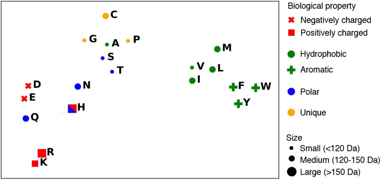
To investigate if the network has learned to encode biochemistry in representations, we project the weight matrix of the final embedding layer of the network into two dimensions with t-SNE (Maaten & Hinton, 2008) and present visualizations in Figure 1. Visual inspection reveals that the representation of amino acids in the network’s embeddings is organized by biochemical properties. Hydrophobic and polar residues are clustered separately, including a tight grouping of the aromatic amino acids Tryptophan (W), Tyrosine (Y), and Phenylalanine (F). The negatively charged amino acids Aspartic Acid (D) and Glutamic Acid (E), as well as the positively charged Arginine (R) and Lysine (K) are respectively paired. Histidine (H), charged or polar depending on its environment, is grouped with the polar residues. The polar amino acid Glutamine (Q) which is structurally similar to both the positively charged Arginine and negatively charged Glutamic Acid lies approximately halfway between the two in the representation space. The three smallest molecular weight amino acids Glycine (G), Alanine (A), and Serine (S) are grouped, as are Hydroxyl-containing Serine (S) and Threonine (T). Cysteine is a relative outlier which might relate to its ability to form disulfide bonds. In this analysis, we omit the infrequently appearing amino acids B (Asparagine), U (Selenocysteine), Z (Glutamine), O (Pyrrolysine) as well as X (the unknown token). We plot representations of the remaining 20 amino acids.

The trained Transformer model encodes amino acid properties in the model’s output embeddings, visualized here with t-SNE. Amino acids cluster in representation space according to biochemistry and molecular weight. The polar amino acid Glutamine (Q) which is structurally similar to both the positively charged Arginine (R) and negatively charged Glutamic Acid (E) lies approximately halfway between the two in the representation space. Histidine (H), polar or positively charged depending on context, can be clustered with either category.
4.2 Embeddings of orthologous proteins
The final hidden representation output by the network is a sequence of vectors, one for each position in the sequence. An embedding of the complete sequence, a vector summary that is invariant to sequence length, can be produced by averaging features across the full length of the sequence. These embeddings represent sequences as points in high dimensional space. Each sequence is represented as a single point and similar sequences are mapped to nearby points.
We investigate organization of the space of protein embeddings using sets of proteins related by orthology. Orthologous genes are corresponding genes between species that have evolved from a common ancestor by speciation. Generally, these genes will have different sequences but retain the same function (Huerta-Cepas et al., 2018).
Similarity-based spatial organization of orthologous genes
Proteins that are related by orthology share a high level of sequence similarity by virtue of their common ancestry. Intrinsic organization in orthology data might be expected from bias in the amino acid compositions of proteins from different species. This similarity is likely to be captured by inductive biases of untrained language models even prior to learning, as well as by the frequency baseline. We find in Figure 2a that the baseline representations show some organization by orthology. Clustering in the LSTM representations and frequency baseline are similar. The untrained Transformer is more clustered than the other baselines. The trained Transformer representations show tight clustering of orthologous genes implying that learning has identified and represented their similarity.

Protein sequence representations encode and organize orthological, species, and phylogentic information of sequences. (a) visualizes representations of several orthologous groups from different species via t-SNE. Sequences from the same orthologous group have the same color. The trained Transformer representations cluster by orthology more densely than do baseline representations. (b) visualizes ortholog sequence representations via PCA (a linear projection technique). Character label denotes species and genes are colored by orthologous group. The trained Transformer representations self-organize along a species axis (horizontal) and orthology axis (vertical), in contrast to baseline representations. (c) visualizes per-species averaged sequence representations along with an overlay of phylogenetic hierarchy (colors represent distinct phyla). Representations are post-processed using a learned hierarchical distance projection. The trained Transformer provides more phylogenetically structured representations than do baselines.
Principal components and directional encoding
We hypothesize that trained models encode similar representations of orthologous genes by encoding information about both orthology and species by direction in the representation vector space. We apply principal component analysis (PCA), to recover principal directions of variation in the representations. If information about species and orthology specify the two main directions of variation in the high dimensional data then they will be recovered in the first two principal components. We select 4 orthologous genes across 4 species to look for directions of variation. Figure 2b indicates that linear dimensionality reduction on trained-model sequence representations recovers species and orthology as the major axes of variation, with the primary (horizontal) axis corresponding to species and the secondary (vertical) axis corresponding to ortholog family. While the baseline representations are often able to cluster sequences by ortholog family, they fail to encode orthology or species information in their orientation.
We note that the principal components of the untrained LSTM representations are oriented almost identically to those of the amino acid frequency representations, suggesting that the LSTM’s inductive bias primarily encodes frequency information. In contrast, the untrained Transformer representation yields a tighter clustering by ortholog family, indicating that the inductive biases of the Transformer model capture higher-order information about sequences even without any learning.
Phylogenetic organization
Just as averaging per-residue representations produces protein embeddings, averaging per-protein embeddings for a subset of the proteins of a species produces species representations. We qualitatively examine the extent to which these representations correspond to phylogeny.
Reusing the set of orthologous groups from above, we generate species representations for 2609 species and subsequently learn a phylogenetic distance projection on the representations along the lines of Hewitt & Manning (2019) 3. Figure 2c, which depicts the projected representations of 48 randomly-selected species evenly split across the three taxonomic domains, suggests that the Transformer species representations cohere strongly with natural phylogenetic organization, in contrast to the LSTM and frequency baselines.
4.3 Translating between proteins in representation space
To quantitatively investigate the learned structural similarities explored above, we assess nearest neighbor recovery under vector similarity queries in the representation space. If biological properties are encoded along independent directions in representation space, then corresponding proteins with a unique biological variation are related by linear vector arithmetic.
We cast the task of measuring the similarity structure of the representation space as a search problem. To perform a translation in representation space, we compute the average representations of proteins belonging to the source and target sets. Then, the difference between these averages defines a direction in representation space, which can be used for vector arithmetic 4. After applying a vector translation to the source, a fast nearest neighbor lookup in the vector space can identify the nearest proteins to the query point. The rate of recovering the target of the query in the nearest neighbor set quantifies directional regularity. We report the top-k recovery rate, the probability that the query target recovers the target protein among its top-k nearest neighbors.
We study two kinds of protein translations in vector space: (1) translations between orthologous groups within the same species and (2) translations between different species within the same orthologous group. Intuitively, if the representation space linearly encodes orthology and species information, then we expect to recover the corresponding proteins with high probability.
Translation between different orthologs of the same species
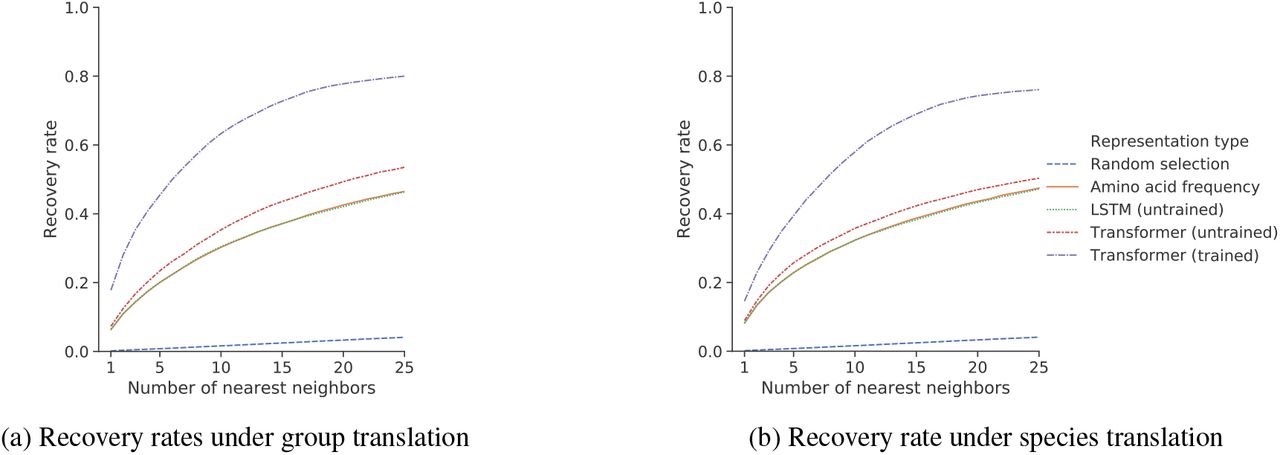
To translate between protein a and protein b of the same species, we define the source and target sets as the average of protein a or protein b across all 24 diverse species. If representation space linearly encodes orthology, then adding the difference in these averages to protein a of some species will recover protein b in the same species. Figure 3a shows recovery rates for the trained model and baselines for randomly selected proteins and pairs of orthologous groups.

Learned sequence representations can be translated between orthologous groups and species. Depicted is the recovery rate of nearest-neighbor search under (a) orthologous group translation, and (b) species translation; in both settings, the trained Transformer representation space has a higher recovery rate.
Translation between corresponding orthologous genes in different species
We use an analogous approach to translate a protein of a source species s to its ortholog in the target species t. Here, we consider the average representation of the proteins in s and in t. If representation space is organized linearly by species, then adding the difference in average representations to a protein in species s will recover the corresponding protein in species t. Figure 3b shows recovery for species translations, finding comparable results to orthologous group translation.
In both translation experiments, representations from the trained Transformer have the highest recovery rates across all values of k, followed by the untrained Transformer baseline. The recovery rate approaches 80% for a reasonable k = 20 (Figure 3b), indicating that information about orthology and species is loosely encoded directionally in the structure of the representation space. The recovery rates for the untrained LSTM and amino acid frequency baselines are nearly identical, supporting the observation that the inductive bias of the LSTM encodes frequency information. Figure 2b visualizes the projected representations of four orthologous groups across four species.
4.4 Learning encodes sequence alignment features
Multiple sequence alignments (MSAs) identify corresponding sites across a family of related sequences (Ekeberg et al., 2013a). These correspondences give a picture of the variation at different sites within the sequence family. The neural network receives as input single sequences and is given no access to family information except via learning. We investigate the possibility that the contextual per-residue representations learned by the network encode information about the family.
One way family information could appear in the network is through assignment of similar representations to positions in different sequences that are aligned in the family’s MSA. Using the collection of MSAs of structurally related sequences in Pfam (Bateman et al., 2013), we compare the distribution of cosine similarities of representations between pairs of residues that are aligned in the family’s MSA to a background distribution of cosine similarities between unaligned pairs of residues. A large difference between the aligned and unaligned distributions implies that self-supervision has developed contextual representations that use shared features for related sites within all the sequences of the family.
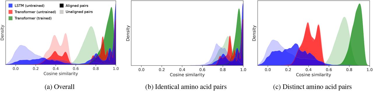
Figure 4a depicts the distribution of cosine similarity values between aligned and unaligned positions within a representative family for the trained model and baselines. A marked shift between aligned and unaligned pairs results from learning. Visually, trained Transformer representations effectively discriminate between aligned and unaligned positions, while the untrained Transformer model is unable to separate the distributions. The untrained LSTM representations show a slight separation of the distributions. We observe in Figure 4b and Figure 4c that these trends hold even under the constraints that the residue pairs (1) share the same amino acid identity or (2) have different amino acid identities.

Per-residue representations from trained models implicitly align sequences. Depicted are distributions of cosine similarity of representations of sequences from within PFAM family PF01010. Note that (a) is an additive composition of (b) and (c). The differences between dark green and light green distributions imply that the trained Transformer representations are a powerful discriminator between aligned and unaligned positions, especially when compared to the baseline representations.
We estimate differences between the aligned and unaligned distributions across 128 Pfam families using the area under the ROC curve (AUC) as a metric of discriminative power between aligned and unaligned pairs. Average AUC is shown for each representation type in (Table 2). The aggregate results demonstrate a shift in the discrimination power across the families from low for the untrained Transformer to high for the trained Transformer caused by learning. These results support the hypothesis that self-supervision is capable of encoding contextual features found by MSA.
Area under the ROC curve (AUC) of per-residue representational cosine similarities in distinguishing between aligned and unaligned pairs of residues within a Pfam family. Results displayed are averaged across 128 families.
5 Emergence of secondary structure and tertiary contacts
5.1 Secondary structure
Structural information likely constitutes part of a minimal code for predicting contextual dependencies in sequence variation. Information about compatibility of a sequence with secondary structure is present in sequence variation, implying that self-supervision may be able to compress variation in its training data through secondary structure features. We use secondary structure prediction accuracy of a linear projection of per-residue representations as a proxy to measure secondary structure information discovered in the course of learning.
We examine final hidden representations for the presence of information about secondary structure at different stages of training. To establish a baseline, we compare to (1) one-hot amino acid representations, which results in the prior that predicts the most likely label for each position’s amino acid, and (2) representations from family-level frequencies summarized in position-specific scoring matrices (“PSSM”s; Jones, 1999) for each protein. The untrained model contains some information about secondary structure above the prior but performs worse than the PSSM features. In the initial stages of training a rapid increase in the information about secondary structure is observed (Figure 5a). A 36-layer Transformer model trained on the full pre-training dataset yields representations that project to 75.5% Q3 (3-class) or 60.8% Q8 (8-class) test accuracy. For calibration, current state-of-the-art on the same dataset is 84 % on the Q3 (3-class) task (Wang et al., 2016) or 70.5% on Q8 (8-class) task (Drori et al., 2018) using a technique considerably more sophisticated than linear projection. Full results for both tasks are presented in Table S1.

Learned representations encode secondary structure information in a linearly recoverable manner. (a) displays top-1 secondary structure prediction test accuracy of trained Transformer representation projections over the course of pre-training, where top depicts accuracy as a function of model pre-training update steps and bottom depicts accuracy as a function of pre-training loss. (b) illustrates the 3-class representation projections on representative proteins (PDB IDs 2DPG and 1BDJ; Cosgrove et al., 1998; Kato et al., 1999) selected for dissimilarity with the training dataset, having sequence identity no higher than 0.274 and 0.314, respectively, with any training sequence. Red denotes helix, green denotes strand, and white denotes coil. Color intensities denote prediction confidence.
Pre-training dataset scale
The amount of information encoded in the learned representation is related to the scale of the data used for training. We examine the effect of pre-training dataset size on the model by training the same model with a randomly chosen subset of 1% of the full pre-training dataset. In doing so, we find a gap reflected both in the relationship between accuracy and number of updates and also in accuracy for the same pre-training loss (Figure 5a). We conclude that two models with the same predictive performance on the self-supervision objective differ in their information content. Specifically, increasing the amount of training data also increases the amount of secondary structure information in the representation, even after controlling for training progress (i.e. for models with the same pre-training validation loss).
Pre-training dataset diversity
To clarify the role that learning across diverse sets of sequences plays in generating representations that contain generalizable structural information, we compare the above setting (training across evolutionary statistics) to training on single protein families. We train separate models on the multiple sequence alignments of the three most common domains in nature longer than 100 amino acids, the ATP-binding domain of the ABC transporters, the protein kinase domain, and the response regulator receiver domain. We test the ability of models trained on one protein family to generalize information within-family and out-of-family by evaluating on sequences with ground truth labels from the family the model was trained on or from the alternate families. In all cases, the model trained on within-family sequences outperforms the models trained on out-of-family sequences (Table 3), indicating poor generalization of training on single MSA families. More significantly, however, the model trained across the full sequence diversity has a higher accuracy than the single-family model accuracies, even on the same-family evaluation dataset. This suggests that the representations learned from the full dataset are capturing general purpose information about secondary structure learned outside the sequence family.
Top-1 secondary structure prediction test accuracy by an optimal linear projection of per-amino-acid vector representations on three PFAM families (PF00005: ATP-binding domain of the ABC transporters; PF00069: Protein kinase domain; PF00072: Response regulator receiver domain). For Transformer models, the pre-training dataset is stated in parentheses. Q3 denotes 3-class prediction task. Underline denotes cases in which the pre-training data comes from the same Pfam family used for evaluation.
5.2 Residue-residue contacts
Spatial contacts between amino acids describe a rotation- and translation-invariant representation of 3-dimensional protein structure. Contacts can be inferred through evolutionary correlations between residues in a sequence family (Marks et al., 2011; Anishchenko et al., 2017). Contacts predicted from evolutionary data have enabled large-scale computational prediction of protein structures (Ovchinnikov et al., 2017). Recently, deep neural networks have shown strong performance on predicting protein contacts and tertiary structure using evolutionary data. For inputs, these methods use raw frequency and covariance statistics, or parameters of maximum-entropy sequence models fitted on MSAs (Jones & Kandathil, 2018; Xu, 2018; Senior et al., 2018). However, these approaches often model structure at the family level and require access to many related sequences (e.g. to construct MSAs). Here we study whether networks trained on full evolutionary diversity have information that can be used to predict tertiary contacts directly from single sequences.
To adapt the Transformer network to predict contacts, we represent interactions between amino acids at positions i and j by a quadratic form in the final hidden representations, h, with learned projections, P and Q, having the network output:

The network parameters are optimized by minimizing the binary cross entropy between wij and the data. To examine if tertiary contact information is linearly encoded in the final hidden representations, we freeze the network parameters and train only the linear projections P and Q of the learned final hidden representations. To confirm that the information is encoded in the representations and not simply a result of good projections, we control the experiment by comparing to a Transformer without pre-training. In this experiment, the pre-trained Transformer performs well (Table 4 and Figure S1), while the control performs worse than a convolutional baseline. Fine-tuning the network end-to-end gives significant additional gains, suggesting that additional information about tertiary structure is distributed throughout the network weights.
Average AUC values on test set by different models for residue-residue contact prediction. These correspond to the average ROC curves shown in Figure S1. Full data and 10% data denote the amount of data used to fine-tune/train different models.
Next, we examine the benefit of pre-training when the fine-tuning dataset is small. We train all models on a randomly chosen subset of 10% of the full fine-tuning dataset. In this limited data regime, the pre-trained models perform significantly better than the non-pretrained or convolutional baseline (Table 4), highlighting the advantage of pre-training when the task data is limited.
Figure 6 shows an example of contacts predicted by the fine-tuned and frozen pre-trained models on the Multiple antibiotic resistance (MarR) protein (PDB: 1JGS; Alekshun et al., 2001), where both models perform well and are able to retrieve most of the long range contacts.
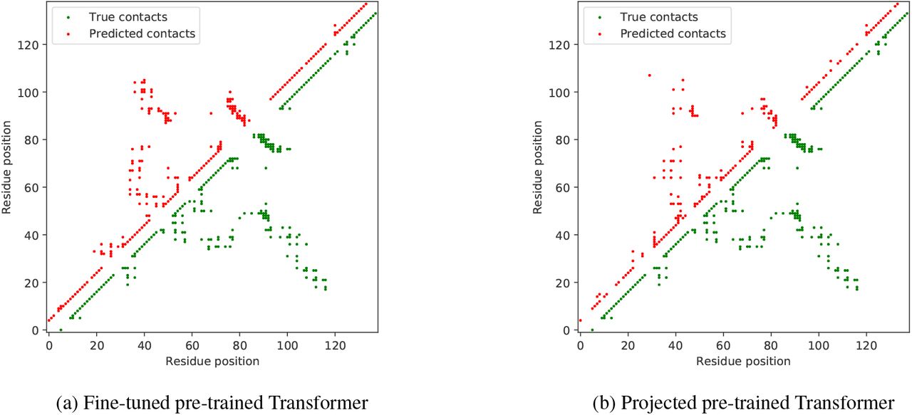
Pre-trained Transformer models accurately predict contacts for chain A of the MarR protein (PDB: 1JGS; Alekshun et al., 2001). Depicted are true contacts along with contacts predicted by (a) fine-tuned pre-trained Transformer, and (b) projected pre-trained Transformer. The MarR protein was selected for its dissimilarity with the training dataset, having a sequence identity no higher than 0.431 with any training sequence.
Long range contacts
We explore performance on tertiary contacts of increasing range of sequence separation. We evaluate mean top-L precision scores (where L is length of a protein sequence) on test data for sequence separations greater than 4, 8, 11, and 23 positions. Results are shown in Figure 7. As expected, precision declines for all models as sequence separation is increased. The contacts predicted by fine-tuning the pre-trained model are consistently more precise than other baselines across contact separation distances. Notably, the projected pre-trained model (which can only make use of information directly present in the final representation) performs better than complete end-to-end training of the Transformer baselines.

Fine-tuning the pre-trained Transformer model predicts longer-range contacts better than other baselines. Depicted are mean top-L precision values for contacts at different minimum sequence separations on test data. The fine-tuned and projected pre-trained Transformers predict long range contacts better than other baselines, suggesting that pre-training extracts residue-residue contact information directly from protein sequences.
6 Learned representations can be adapted to predict mutational effects on protein function
The mutational fitness landscape provides deep insight into biology: determining protein activity (Fowler & Fields, 2014), linking genetic variation to human health (Lek et al., 2016; Bycroft et al., 2018; Karczewski et al., 2019), and enabling for rational protein engineering (Slaymaker et al., 2016). For synthetic biology, iteratively querying a model of the mutational fitness landscape could help efficiently guide the introduction of mutations to enhance protein function (Romero & Arnold, 2009), inform protein design using a combination of activating mutants (Hu et al., 2018), and make rational substitutions to optimize protein properties such as substrate specificity (Packer et al., 2017), stability (Tan et al., 2014), and binding (Ricatti et al., 2019).
Computational variant effect predictors are useful for assessing the effect of point mutations (Gray et al., 2018; Adzhubei et al., 2013; Kumar et al., 2009; Hecht et al., 2015; Rentzsch et al., 2018). Their predictions are based on basic evolutionary, physiochemical, and structural protein features that have been selected for their relevance to protein activity. However, features derived from evolutionary homology are not available for all proteins; and protein structural features are only available for a small fraction of proteins.
Building on the finding that unsupervised learning causes knowledge of intrinsic protein properties to develop in the internal representations of the Transformer – including biochemical, structural, and homology information relevant to protein molecular function – we adapt the representations to predict the quantitative effect of mutations.
Fine-tuning the Transformer with labeled variant activity data yields a variant effect predictor with performance matching Envision (Gray et al., 2018), a state-of-the-art predictor, in a direct comparison. The Transformer predictions are more general and can be applied to proteins that are missing features required by other variant predictors.
Coupling next generation sequencing with a mutagenesis screen enables parallel readout of tens of thousands of variants of a single protein (Fowler & Fields, 2014). This data is a valuable enabler for machine learning protein biology. Recently, Gray et al. (2018) combined over 20,000 variant effect measurements from nine large-scale experimental mutagenesis datasets to train Envision, a supervised model of the effect of missense mutations on protein activity. We train on the same data and compare Envision’s predictions using its standard input features to the Transformer, which predicts from raw sequences alone.
Intra-protein variant effect prediction
Following the approach used in Gray et al. (2018), for each protein a fraction p = 0.8 of the data is used for training and the remaining data is used for testing (Figure 8a). For this experiment, we report the result of 5-fold cross-validation. There are minimal deviations across each run. When using 80% of the data for training, standard deviations in Spearman ρ are < 0.06 for each protein task (Table S2).

After pre-training, the Transformer model can be adapted to predict mutational effects on protein function. A 12 layer pre-trained Transformer model was fine-tuned on mutagenesis data. (a) compares the best model to Gray et al. (2018), where both models use 80% of the data for training. (b) shows performance on various proteins when training on smaller data subsets.
The Transformer exceeds the performance of the Gray et al. (2018) baseline on 10 of the 12 proteins. Of the twelve assays modeled in their study, the Brca1 RING domain and E4B ubiquitin ligase were reported to be difficult due to missing structural features; low correlation between features and variant effect scores; or incomplete functional information (Gray et al., 2018). The Transformer is able to accurately predict mutational effects on these proteins (Figure 8a).
Fine-tuning on minimal data
We also evaluate the performance of the fine-tuned Transformer in a limited data regime. For each protein, we vary the fraction p ∈ {0.8, 0.5, 0.3, 0.1, 0.01} of data that is used for training. We find that 86% and 40% of final performance can be achieved by training on just 30% or 1% of the data respectively (Figure 8b). As the average number of mutants tested per protein is 2379, this corresponds to training on data from < 25 mutants on average.
Generalization to held-out proteins
We analyze the Transformer’s ability to generalize between proteins by performing a leave-one-protein-out (LOPO) analysis, as was proposed in Gray et al. (2018). To evaluate performance on a given protein, we train on data from the remaining n − 1 proteins and test on the held-out protein. Figure 9 shows that the Transformer’s predictions from raw sequences perform better on 5 of the 9 tasks assessed by Gray et al. (2018).

Best model vs. Gray et al. (2018) on leave-one-out-protein (LOPO) tasks. For both models, the averages were computed across all proteins shown excluding E4B, BRCA1 (E3 ligase activity), and BRCA1 (Bard1 binding), as Gray et al. (2018) did not include these in LOPO analysis, due to poor performance on the intra-protein cross-validation task.
These results show that the intrinsic knowledge of proteins discovered by self-supervision on large-scale protein data generalizes to predicting protein functional activity; and that the features developed through this learning – which are available for all proteins because they are from raw sequences – can be used to match performance of a state-of-the-art variant effect predictor that makes use of powerful structural and evolutionary feature inputs.
7 Discussion
One of the goals for artificial intelligence in biology could be the creation of controllable predictive and generative models that can read and generate biology in its native language. Accordingly, research will be necessary into methods that can learn intrinsic biological properties directly from protein sequences, which can be transferred to prediction and generation.
We investigated deep learning across evolution at the scale of the largest available protein sequence databases, training contextual language models across 86 billion amino acids from 250 million sequences. The space of representations learned from sequences by high-capacity networks reflects biological structure at many levels, including that of amino acids, proteins, groups of orthologous genes, and species. Information about secondary and tertiary structure is internalized and represented within the network in a generalizable form.
This information emerges without supervision – no learning signal other than sequences is given during training. We find that networks that have been trained across evolutionary data generalize: information can be extracted from representations by linear projections or by adapting the model using supervision. It is possible to adapt networks that have learned on evolutionary data to give results matching state-of-the-art on variant activity prediction directly from sequence – using only features that have been learned from sequences and without evolutionary and structural prior knowledge.
While the contextual language models we use are comparable with respect to data and capacity to large models studied in the literature for textual data, our experiments have not yet reached the limit of scale. We observed that even the highest capacity models we trained (with approximately 700M parameters) underfit the 250M sequences, due to insufficient model capacity. The relationship we find between the information in the learned representations and predictive ability in the self-supervision task suggests that higher capacity models will yield better representations.
Combining high-capacity generative models with gene synthesis and high throughput characterization can enable generative biology. The network architectures we have trained can be used to generate new sequences (Wang & Cho, 2019). If neural networks can transfer knowledge learned from protein sequences to design functional proteins, this could be coupled with predictive models to jointly generate and optimize sequences for desired functions. The size of current sequence data and its projected growth point toward the possibility of a general purpose generative model that can condense the totality of sequence statistics, internalizing and integrating fundamental chemical and biological concepts including structure, function, activity, localization, binding, and dynamics, to generate new sequences that have not been seen before in nature but that are biologically active.
A Approach & Data
A.1 Background on language models and embeddings
Deep language models are parametric functions that map sequences into distributed word representations in a learned vector space (Bengio et al., 2003; Mikolov et al., 2013a;b; Pennington et al., 2014; Lample et al., 2017). These vectors, called embeddings, distribute the meaning of the source sequence across multiple components of the vector, such that semantically similar objects are mapped to nearby vectors in representation space.
Recently, exciting results of large-scale pre-trained language models have advanced the field of natural language processing and impacted the broader deep learning community. Peters et al. (2018) used a coupled language model objective to train bidirectional LSTMs in order to extract context dependent word embeddings. These embeddings showed improvement for a range of NLP tasks. Radford et al. (2018) explored a semi-supervised method using left-to-right Transformer models to learn universal representations using unsupervised pre-training, followed by fine-tuning on specific downstream tasks. Recently, Devlin et al. (2018) proposed BERT to pre-train deep representations using bidirectional Transformer models. They proposed a pre-training objective based on masked language modeling, which allowed capturing both left and right contexts to obtain deep bidirectional token representations, and obtained state-of-the-art results on 11 downstream language understanding tasks, such as question answering and natural language inference, without substantial task-specific architecture modifications. Radford et al. (2019) extended their earlier work and proposed GPT-2, highlighting the importance of scale along dimensions of number of model parameters and size of pre-training data, and demonstrated their learned language model is able to achieve surprisingly good results on various NLP tasks without task-specific training. Analogous follow-up work on other domains have also shown promising results (Sun et al., 2019).
A.2 Model Architecture
We use a deep bidirectional Transformer encoder model (Devlin et al., 2018; Vaswani et al., 2017) and process data at the character-level, corresponding to individual amino-acids in our application. In contrast to models that are based on recurrent or convolutional neural networks, the Transformer makes no assumptions on the ordering of the input and instead uses position embeddings. Particularly relevant to protein sequences is the Transformer’s natural ability to model long range dependencies, which are not effectively captured by RNNs or LSTMs (Khandelwal et al., 2018). One key factor affecting the performance of LSTMs on these tasks is the path lengths that must be traversed by forward activation and backward gradient signals in the network (Hochreiter et al., 2001). It is well known that structural properties of protein sequences are reflected in long-range dependencies (Kihara, 2005). Classical methods that aim to detect pairwise dependencies in multiple sequence alignments are able to model entire sequences. Similarly, the Transformer builds up a representation of a sequence by alternating self attention with non-linear projections. Self attention structures computation so that each position is represented by a weighted sum of the other positions in the sequence. The attention weights are computed dynamically and allow each position to choose what information from the rest of the sequence to integrate at every computation step. Developed to model large contexts and long range dependencies in language data, self-attention architectures currently give state-of-the-art performance on various natural language tasks, mostly due to the Transformer’s scalability in parameters and the amount of context it can integrate (Devlin et al., 2018). The tasks include token-level tasks like part-of-speech tagging, sentence-level tasks such as textual entailment, and paragraph-level tasks like question-answering.
Each symbol in the raw input sequence is represented as a 1-hot vector of dimension 25, which is then passed through a learned embedding layer before being presented to the first Transformer layer. The Transformer consists of a series of layers, each comprised of (i) multi-head scaled dot product attention and (ii) a multilayer feed-forward network. In (i) a layer normalization operation (Ba et al., 2016) is applied to the embedding, before it undergoes three separate linear projections via learned weights (distinct for each head) Wq, Wk, Wv to produce query q, key k and valve v vectors. These vectors from all positions in the sequence are stacked into corresponding matrices Q, K and V. The output of a single head is  . V, where dk is the dimensionality of the projection. This operation ensures that each position in the sequence attends to all other positions. The outputs from multiple heads are then concatenated. This output is summed with a residual tensor from before (i) and is passed to (ii). In (ii), another layer normalization operation is applied and the output is passed through a multi-layer feed-forward network with ReLU activation (Nair & Hinton, 2010) and summed with a residual tensor from before (ii). This result is an intermediate embedding for each position of the input sequence and is then passed to the next layer. Thus, the overall network takes a sequence as input and outputs a sequence of vectors forming a distributed representation of the input sequence which we refer to as the final representation for the sequence. The parameters of the model are the weight matrices Wq, Wk, Wv for each layer and attention head; the weights of the feedforward network in each layer/head and the batch norm scale/shift parameters. The training procedure for these weights is detailed in Appendix A.3.
In our work, we experimented with Transformer models of various depths, including a 36 layer Transformer with 708.6 million parameters (Table 5). All models were trained using the fairseq toolkit (Ott et al., 2019) on 128 NVIDIA V100 GPUs for  days with sinusoidal positional embeddings (Vaswani et al., 2017), without layer norm in the final layer, and using half precision. The 36 and 24 layer models were trained with initializations from Radford et al. (2019), while the 12 layer model was trained with initializations from Vaswani et al. (2017). Batch size was approximately 2500 sequences for each model.
Hyperparameters for Transformer models trained in this paper. Embedding dim refers to the amino acid representation dimensionality. MLP dim refers to the width of hidden layers in the Transformer’s MLPs. (A) refers to the number of pre-training steps before analyzing secondary structure. (B) gives the number of pre-training steps before visualizations were performed and fine-tuning on tertiary structure and protein mutagenesis data was conducted.
A.3 Pre-training the models
During unsupervised pre-training, the final high dimensional sequence representations are projected, via a linear layer, to vectors of unnormalized log probabilities. These probabilities correspond to the model’s posterior estimate that a given amino acid is at that position, given all other amino acids in the sequence. These estimates are optimized using a masked language model objective. We follow the masking procedure from Devlin et al. (2018) in which the network is trained by noising (either by masking out or randomly perturbing) a fraction of its inputs and optimizing the network to predict the amino acid at the noised position from the complete noised sequence. In contrast to Devlin et al. (2018), we do not use any additional auxiliary prediction losses.
Protein sequence pre-training data
We train on the full Uniparc dataset (The UniProt Consortium, 2007) without any form of preprocessing or data cleaning. This dataset contains 250 million sequences comprising 86 billion amino acids. For context, other recently published language modeling work includes Radford et al. (2019), who used 40GB of internet text or roughly 40 billion characters; Baevski et al. (2019), who used 18 billion words; and Jozefowicz et al. (2016), who used 100 billion words.
We constructed a “full data” split by partitioning the full dataset into 249M training and 1M validation examples. We subsampled the 249M training split to construct three non-overlapping “limited data” training sets with 10%, 1%, and 0.1% data, which consist of 24M, 2M and 240k sequences respectively. The validation set used for these “limited data” experiments was the same as in the “full data” split.
The 24 layer and 12 layer Transformer models were trained on a different split of the full dataset, with 225M sequences randomly selected for training and the remaining 25M sequences used for validation.
Pre-training task
The pre-training task follows Task #1 in Section 3.3.1 of Devlin et al. (2018). Specifically, we select as supervision 15% of tokens randomly sampled from the sequence. For those 15% of tokens, we change the input token to a special “masking” token with 80% probability, a randomly-chosen alternate amino acid token with 10% probability, and the original input token (i.e. no change) with 10% probability. We take the loss to be the whole batch average cross entropy loss between the model’s predictions and the true token for these 15% of amino acid tokens. We then report the mean exponentiated cross-entropy (ECE) for the various models trained, as shown in Table 1.
Pre-training details
Our model was pre-trained using a context size of 1024 tokens. As most Uniparc sequences (96.7%) contain fewer than 1024 amino acids, the Transformer is able to model the entire context in a single model pass. For those sequences that are longer than 1024 tokens, we sampled a random crop of 1024 tokens during each training epoch. The model was optimized using Adam (β1 = 0.9, β2 = 0.999) with learning rate 1e − 4. The models follow a warm-up period of 16000 updates, during which the learning rate increases linearly. Afterwards, the learning rate follows an inverse square root decay schedule. The number of pre-training steps is listed in Table 5.
A.4 Baselines
In addition to comparing to past work, we also implemented a variety of deep learning baselines for our experiments.
Frequency (n-gram) models
To establish a meaningful performance baseline on the sequence modeling task (Section 3), we construct n-gram frequency-based models for context sizes 1 ≤ n ≤ 104, applying optimal Laplace smoothing for each context size. The Laplace smoothing hyperparameter in each case was tuned on the validation set. Both unidirectional (left conditioning) and bidirectional (left and right conditioning) variants are used.
Recurrent neural networks
For this baseline (applied throughout Section 4), we embedded the amino acids to a representation of dimension 512 and applied a single layer recurrent neural network with long-short term memory (LSTM) with hidden dimension 1280.
Convolutional neural networks
For residue-residue contact prediction (Section 5.2), we trained convolution baselines where we embedded the amino acids to a representation of dimension k, resulting in a k × N image (where N is the sequence length). We then applied a convolutional layer with C filters and kernel size M followed by a multilayer perceptron with hidden size D. We tried different values of k, C, M and D, to get best performing models. The model was trained using Adam with β1 = 0.9, β2 = 0.999 and fixed learning rate = 1e−4.
Ablations on Transformer model
To investigate the importance of pre-training, we compared to a Transformer with random weights (i.e. using the same random initializations as the pre-trained models, but without performing any training) for the analyses in Section 4 and Section 5. In Section 5, we refer to these baselines as “no pre-training”, and elsewhere, we refer to these baselines as “untrained”. Separately, to assess the effect of full network fine-tuning, we tested Transformer models where all weights outside task-specific layers are frozen during fine-tuning for the analysis in Section 5.2. In these “projected” baselines, none of the base Transformer parameters are modified during fine-tuning.
A.5 Representational similarity-based alignment of sequences within MSA families
Family selection
For the analysis in Section 4.4, we selected structural families from the Pfam database (Bateman et al., 2013). We first filtered out any families whose longest sequence is less than 32 residues or greater than 1024 residues in length. We then ranked the families by the number of sequences contained in each family and selected the 128 largest families and associated MSAs. Finally, we reduced the size of each family to 128 sequences by uniform random sampling.
Aligned pair distribution
For each family, we construct an empirical distribution of aligned residue pairs by enumerating all pairs of positions and indices that are aligned within the MSA and uniformly sampling 50000 pairs.
Unaligned pair distribution
We also construct for each family a background empirical distribution of unaligned residue pairs. This background distribution needs to control for within-sequence position, since the residues of two sequences that have been aligned in an MSA are likely to occupy similar positions within their respective unaligned source sequences. Without controlling for this bias, a difference in the distributions of aligned and unaligned pairs could arise from representations encoding positional information rather than actual context. We control for this effect by sampling from the unaligned-pair distribution in proportion to the observed positional differences from the aligned-pair distribution. Specifically, the following process is repeated for each pair in the empirical aligned distribution:
Calculate the absolute value of the difference of each residue’s within-sequence positions in the aligned pair.
Select a pair of sequences at random.
For that pair of sequences, select a pair of residues at random whose absolute value of positional difference equals the one calculated above.
Verify that the residues are unaligned in the MSA; if so, add the pair to the empirical background distribution.
Otherwise, return to step 2.
This procedure suffices to compute a empirical background distribution of 50000 unaligned residue pairs.
Similarity distributions
Finally, for each family and each distribution, we apply the cosine similarity operator to each pair of residues to obtain the per-family aligned and unaligned distribution of representational cosine similarities.
Area under the ROC curve
Area under the ROC curve is commonly used to measure the performance of classification problem at various thresholds settings. ROC is a probability curve illustrating the relationship between true positive rate and false positive rate for a binary classification task, and AUC represents degree or measure of separability. It quantifies the model’s capability of distinguishing between classes. Here, we use cosine similarity scores as outputs of a classifier aimed at differentiate between aligned and unaligned pairs.
A.6 Orthology visualations
Full orthology dataset
For the analyses in Section 4, an orthologous group dataset was constructed from eggNOG 5.0 (Huerta-Cepas et al., 2018) by selecting 25 COG orthologous groups toward maximizing the size of the intersected set of species within each orthologous group. Through a greedy algorithm, we selected 25 COG groups with an intersecting set of 2609 species. This dataset was used directly in Section 4.2’s phylogenetic organization analysis.
Diverse orthology dataset
For all analyses in Section 4 besides the aforementioned phylogenetic organization analysis, we shrank the dataset above by selecting only one species from each of 24 phyla in order to ensure species-level diversity.
Phylogenetic distance projection
To learn the distance projection used in the phylogenetic organization analysis, we applied an adapted version of the technique of Hewitt & Manning (2019), originally employed toward learning a natural language parse-tree encoding; we modify the technique to instead learn a phylogenetic tree encoding. We optimize a fixed-size projection matrix B toward the following minimization objective:
 where si and sj denote species within the dataset, d(si, sj) denotes a pairwise distance kernel between two species, and r(s) denotes the representation of species s.
In this analysis, we define the species representation r(s) to be an average of the representations of the species’ sequences within the dataset. We also define the distance kernel as follows:
 where LCA denotes the height of the least common ancestor of species si and sj in the phylogenetic tree. We found the optimal projection via mini-batch stochastic gradient descent, which quickly converges on this objective and dataset.
A.7 Vector-based protein search
For the analysis in Section 4.3, we define various translation operations on the representation space of the diverse orthology dataset described above. Notationally, we use s to denote a single sequence, r(s) to denote a representation of a sequence, 𝔾 to denote an orthologous group, and 𝕊 to denote a species. Both 𝔾 and 𝕊 are considered to be collections containing individual sequences.
Orthologous group translation
For a given sequence representation function r, we define a group mean translation  on a sequence s from orthologous group 𝔾 to group 𝔾′ as follows:

This translation subtracts from r(s) the averaged sequence representation across all sequences in orthologous group 𝔾 and subsequently adds the averaged sequence representation across all sequences in group 𝔾′. Intuitively, when 𝔾 is the orthologous group containing sequence s, one might expect a representation that linearly encodes orthology and species information to better “recover” the sequence belonging to the same species and group 𝔾′. We formally quantify this as top-k recovery rate, which is the probability with which a sequence undergoing group mean translation from its orthologous group 𝔾 to a randomly selected group 𝔾′ ≠ 𝔾 recovers amongst its top k nearest neighbors (under L2 norm in representation space) the sequence corresponding to the same species and to orthologous group 𝔾′.
Orthologous species translation
For completeness, the analogous operation of species mean translation  on a sequence s from species 𝕊 to species 𝕊′ is defined as follows:

Here, the top-k recovery rate is defined as the probability with which a sequence undergoing species mean translation from its species 𝕊 to a randomly selected species 𝕊′ = 𝕊 recovers amongst its top k nearest neighbors the sequence corresponding to the same orthologous group and to different species 𝕊′.
Implementation
We used the Faiss similarity search engine (Johnson et al., 2017) to calculate the top-k recovery rates for both types of translations, for 1 ≤ k ≤ 25.
A.8 Secondary structure projections
For the analysis in Section 5.1, we derived and evaluated optimal linear projections of per-residue representations as follows.
Secondary structure data
To evaluate representations of secondary structure in the model, we used a training dataset pre-processed by Zhou & Troyanskaya (2014), which is based on the PISCES Cull PDB database. This dataset, labeled 5926_filtered by the authors, contains the amino acid identities, Q8 (8-class) secondary structure labels, family-level frequency profiles, and miscellaneous other attributes for 5365 protein sequences.
As our test dataset, we used the CB513 dataset, also as preprocessed by Zhou & Troyanskaya (2014).
Linear projection technique
For each representation type, the optimal linear projection for secondary structure prediction was derived via multiclass logistic regression from the per-residue representation vectors to the secondary structure labels, with residues aggregated across all sequences in the training dataset.
Single-family data and analysis
For each of the three domains used, we extracted all domain sequences from the Pfam dataset (Bateman et al., 2013) and located the subset of PDB files containing the domain, using the latter to derive ground truth secondary structure labels (Kabsch & Sander, 1983).
Pre-training follows the methodology of Appendix A.3, except that the datasets were from the domain sequences rather than Uniparc sequences. The domain sequences were randomly partitioned into training, validation, and testing datasets. For each family, the training dataset comprises 65536 sequences, the validation dataset comprises either 16384 sequences (PF00005 and PF00069) or 8192 sequences (PF00072), and the test dataset comprises the remainder.
Each Pfam family also forms an evaluation (projection) dataset; from the sequences with corresponding crystal structures, the training dataset comprises 80 sequences and the test dataset comprises the remainder.
A.9 Fine-tuning procedure
After pre-training the model with unsupervised learning, we can adapt the parameters to supervised tasks. By passing the inputs through our pre-trained model, we obtain a final vector representation of the input sequence h. During pre-training, this representation is projected to a predicted distribution l. Recall that a softmax over l represents the model’s posterior for the amino acid at that position. These final representations are fine-tuned in a task-dependent way.
A.9.1 Tertiary contacts
Tertiary contact data
For the analysis in Section 5.2, we derived a dataset based on the S40 subset in the non-redundant datasets in CATH (Orengo et al., 1997). The S40 subset has only those sequences where any pair of domains shares < 40% of sequence identity. The contacts and sequence information were extracted using the PDB files in the S40 subset. The total number of PDB-chain-id files in this subset is 30744. In order to derive the dataset we extracted sequence and contact information. The sequence information was derived using the information in the PDB files. The list of contacts was extracted following a standard criterion used in the literature (Jones et al., 2011), where a contact is defined as any pair of residues where the C−β to C−β distance (C−α to C−α distance in the case of glycine) is < 8 Å, and the residues are at least 4 amino-acids apart in the original sequence. We split each protein chain into one or more contiguous subsequences, which resulted in 66243 total number of [sequence, contact_list] data points. We shuffled the data and selected 80% for train, 10% for validation, and 10% for test data. Under this split, all contiguous subsequences from the same PDB-id were placed in the same set. This resulted in 6505 validation examples and 6846 test examples.
Fine-tuning procedure
To fine-tune the model to predict tertiary contacts, the final representation h was projected to a 512 dimensional vector. Since a N × N contact map has to be predicted, the N × 512 dimensional tensor is first split into two tensors, each with shapes N × 256. This is followed by a matrix outer product of the split tensors to obtain a N × N tensor. We found rescaling the predicted tensor by dividing by  to be helpful in achieving higher accuracy.
A.9.2 Mutagenesis
Mutagenesis data
For the analysis in Section 6, we used a collection of 21,026 variant effect measurements from nine experimental mutagenesis datasets. We used the data originally collected, collated and normalized by Gray et al. (2018). They used this data to train a machine learning model based on features that incorporate expert knowledge of relevant biochemical, structural, and evolutionary features. We use this model as a baseline.
Fine-tuning procedure
To fine-tune the model to predict the effect of changing a single amino acid (e.g. for mutagenesis prediction), we regress  to the scaled mutational effect where π maps an amino acid to its corresponding index; mt AA is the mutant amino acid; and wt AA is the wildtype amino acid. As an evaluation metric, we report the Spearman ρ between the model’s predictions and known values.
Acknowledgments
We thank Tristan Bepler, Yilun Du, Anika Gupta, Omer Levy, Ethan Perez, Neville Sanjana, and Emily Wang for insightful comments and discussions in the course of this work. Furthermore we express our appreciation toward Ian Peikon for providing valuable and creative feedback on multiple iterations of the manuscript.
Footnotes
↵1 In traditional autogressive language modeling, ECE corresponds to the commonly-used perplexity metric.
↵2 Details on the model architecture, data, and training hyperparameters are presented in Appendix A.3.
↵3 See Appendix A.6 for full details of the learned projection.
↵4 See Appendix A.7 for full details of the sequence representation translations.
References


