

Abstract
Numerical classification methods provide essential tools for data analysis in various fields of science. Reallocation algorithms are used for improving an a priori clustering (either a random clustering, or one obtained by another method) by changing iteratively the assignment of objects with the purpose of optimizing a cluster validity criterion. We present two new reallocation algorithms, REMOS1 and REMOS2, which optimize the silhouette width of the objects. REMOS algorithms reallocate ‘misclassified’ objects to their closest cluster; therefore, they increase the overall mean silhouette width of the classification. We compare REMOS algorithms with the recently introduced OPTSIL (Roberts 2015) method from two aspects of performance: optimization efficiency and runtime. We conclude that REMOS algorithms reach similar or higher mean silhouette widths for the final classification, while requiring much shorter computation time.
Introduction
Numerical classification methods are essential data analytical tools in several scientific fields, including ecology, genomics, psychology, or sociology. Basically, classification algorithms can be divided into two groups. Hierarchical algorithms produce a perfectly nested hierarchy of clusters of objects, while the output of non-hierarchical methods is a partition in which each classified object is assigned exclusively to one cluster (or, in the special case of fuzzy clustering methods, non-exclusively to several clusters using fuzzy membership weights) at the same level. Hierarchical methods can be subdivided into agglomerative and divisive methods based on whether they initiate the clustering algorithm from treating each single object as a separate cluster, and then merge them until all objects are included in a single cluster at the highest hierarchical level, or they proceed in the opposite direction by dividing the entire sample iteratively into smaller and smaller subsets in a nested way. The diversity of numerical classification methods is reviewed by several authors, e.g. Kaufman & Rousseeuw (1990), Podani (2000), Peet & Roberts (2013), Legendre & Legendre (2012).
The advantage of hierarchical methods is that they do not need a pre-defined cluster number and their result is unique, while non-hierarchical methods start from an initial classification and improve it iteratively, thus sometimes they converge to a local optimum resulting in a dependence between the initial and the final classification. On the other hand, a disadvantage of hierarchical methods is that earlier steps (either merging or division) constrain further ones, hence the final solution may be suboptimal. In such a case the a posteriori reallocation of misclassified objects might be necessary.
Recently Roberts (2015) introduced two reallocation-based methods which can be used for improving already existing classifications by optimizing a pre-selected goodness criterion. One of these two, called OPTSIL, optimizes the silhouette width which is a widely used index for evaluating classifications and identifying ‘core’ and misclassified objects individually (Rousseeuw 1987, Kaufman & Rousseeuw 1997). Let i be a focal object belonging to cluster A. Let C be a cluster not containing i. a(i) is defined as the average dissimilarity between i and all other objects in A, while c(i,C) is the average dissimilarity between i and all objects in C.

That is, b(i) is the average dissimilarity between i and the members of its closest neighbour cluster. The silhouette width, S(i), is defined as:

S(i) ranges between −1 and +1. Values near +1 indicate that object i is much closer to other objects in the same cluster than to objects of the second closest cluster, implying a correct classification. If s(i) is near 0, the correct classification of the focal object is doubtful, thus suggesting intermediate position between two clusters. S(i) near-1 indicates obvious misclassification. In each iterations, OPTSIL evaluates how much the reallocation of any single object in the classification increases the sample-wise mean of silhouette width. It is done by re-assigning each object from its current cluster to its closest neighbour, and then re-calculating the silhouette widths for all objects. The reallocation which causes the highest increase in the sample-wise mean silhouette is accepted in each step, until no further improvement is possible. Roberts (2015) concluded that OPTSIL is able to significantly improve the initial classification; however, it is extremely time-consuming, thus it is recommended only for ‘polishing’ of classifications made by other methods on small data sets.
We present two silhouette-based reallocation algorithms, called REMOS (Reallocation of Misclassified Objects based on Silhouette width), which are able to improve initial classifications with similar efficiency as OPTSIL while requiring significantly less computation time.
Materials and Methods
The REMOS algorithms
Instead of evaluating the effect of the reallocation of each object on the mean silhouette width, REMOS algorithms simply reallocate one or all of the misclassified objects (i.e. those which have negative silhouette width). According to how objects to reallocate are selected, we introduce two variants of REMOS. REMOS1 reallocates only the object with the most negative silhouette width (i.e., the ‘worst classified’ object), while REMOS2 reallocates all objects with negative silhouette width (i.e., all misclassified objects). Both algorithms stop if the lowest silhouette width reaches a threshold L, or if no further improvement is possible due to a cycle in the iteration. By default L is 0; however, using different values between −1 and 0 can control tolerance towards misclassifications. The steps of the algorithms are presented below:
Calculating the silhouette widths, S(i), for the classified objects;
Are there any objects with S(i) < L?
2a. If no, then go to (5)
2b. If yes, go to (3)
Updating the classification by reallocating objects:
REMOS1: reallocate only the object with the lowest silhouette width to its neighbour cluster;
REMOS2: reallocate all the objects with S(i) < L to their respective neighbour clusters;
Go to (1).
End – no further optimization is possible
Our preliminary runs showed that both REMOS algorithms frequently converge into loops where the iteration proceeds repeatedly over a finite number of suboptimal solutions without finding any of them as a final solution. To break such a loop, we included a test which checks the last 10 iterations and if there are two equal values of mean silhouette width within this range, the solution leading to the highest mean silhouette width is accepted as final. An R script of the REMOS algorithms is provided in the Supplementary material.
Data sets
We compared the performance of the REMOS1, REMOS2 and the OPTSIL algorithms on a real and an artificial data set. As real data example, we used the Grasslands data set that was also applied by Lengyel et al. (2018). This data set contains phytosociological relevés collected on unproductive to moderately productive, mesic pastures, hay meadows, and recently abandoned grasslands of northern Hungary. Species abundances are coded on percentage scale. Grassland subtypes included in this sample cannot be sharply differentiated (Lengyel et al. 2016); however, using the same abundance transformation and dissimilarity measure as applied here (see Data analysis) Lengyel et al. (2018) identified the four-cluster level as the most stable. As artificial data, we applied a simulated data set of 500 points in two dimensions. The points are aggregated into six fuzzy clusters (Fig. 1). For different test scenarios, its random subsets of different size were used.

The artificial data set containing 500 points in six aggregations
Data analysis
The influence of the number of clusters and the sample size on the performance of the REMOS and OPTSIL algorithms was evaluated from two aspects: optimization success and time efficiency. The effect of the number of clusters was tested on the Grassland data set and on a random subset containing 50 points from the artificial data set. Each sample was subject to the same general analytical protocol starting with calculating a distance matrix of the objects. In case of the Grassland data set, we used the Marczewski-Steinhaus index (Podani 2000) calculated on square-root transformed species cover percentages, while for artificial data Euclidean distance was applied. Then, the distance matrix was submitted for clustering using the partitioning around medoids method (PAM; Kaufman & Rousseeuw 1990). This classification could have been optimized by the three reallocation methods immediately; however, in many cases the PAM classification was ‘too good’ for further improvement, thus it did not allow us to differentiate between the reallocation methods (results not shown). Another option would have been to initiate the optimization procedure from a completely random classification but this was discouraged by Roberts (2015) in case of OPTSIL due to the slowness of the process. As a compromise, we added some amount of noise to the PAM classification by re-assigning 10% of the plots randomly. Plots to re-assign were also selected randomly. This classification (PAM + noise) was optimized by the REMOS1, REMOS2, and OPTSIL methods. PAM was run with increasing number of clusters between two and ten. We used the mean silhouette width (MSW) as validity criterion. The analyses were repeated 50 times to provide a statistically representative distribution of values for MSW. During each run, the runtime of different methods was measured.
For testing the effect of sample size, random subsamples containing 50, 100, 200, and 500 points were drawn from the artificial data set. This subsample was classified into six clusters by PAM, then, as above, cluster memberships of 10% of the points were randomly changed. This classification was used for initiating the optimization algorithms, which were repeated 50 times. The change of mean silhouette width and runtime with increasing sample size was compared between REMOS1, REMOS2, and OPTSIL algorithms.
The data analysis was carried out in the R software environment. Program codes of REMOS1 and REMOS2 are supplied in the Electronic Appendix. OPTSIL was calculated using the optpart package. All calculation were done in the R software environment (R Core Team 2017) using cluster (Maechler et al. 2018), tidyr (Wickham & Henry 2018) and ggplot2 (Wickham 2016) add-on packages.
Results
In Grassland dataset, at the level of two clusters, OPTSIL reached higher mean silhouette widths than REMOS algorithms; however, as the number of clusters increased, REMOS1 gradually became superior, while REMOS2 acquired similar MSW values as OPTSIL (Fig. 2).

The change of mean silhouette width along increasing number of clusters for the three optimization methods in case of the Grassland data set
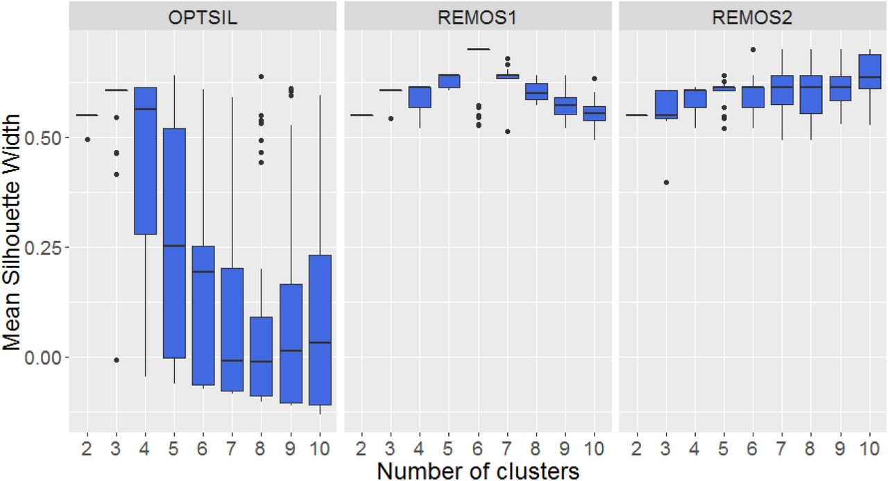
With the artificial data set and two or three clusters, all methods reached solutions with similarly high MSW (Fig. 3). As the number of clusters increased, lower MSW values became dominant with OPTSIL, and, notably, the variation of MSW increased significantly. REMOS1 provided classifications which reached consistently high MSW values, and a peak was experienced at six clusters, which was the correct number of point aggregations. REMOS2 also produced classifications with similarly high MSW with low variation; although, it failed to detect the correct number of clusters. A monotonic trend of increasing MSW with increasing number of clusters was visible in case of REMOS2.

The change of mean silhouette width along increasing number of clusters for the three optimization methods in case of a subsample of the artificial data set
There were differences of several magnitudes between the three methods in runtime. OPTSIL needed less than 1 s with two clusters to optimize; however, as the number of clusters increased, runtimes also did so until reaching a median of 10 s with ten clusters. REMOS1 showed a shallower increment along the number of clusters with runtimes remaining near the magnitude of seconds. REMOS2 was the fastest regardless of the number of clusters with the tested settings, and its median runtimes ranged below or near 0.1 s.
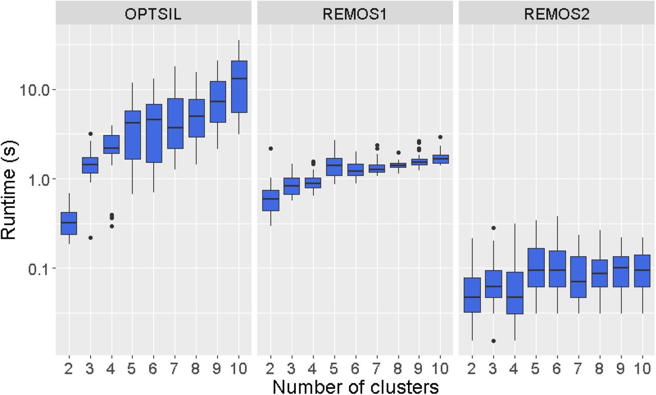
The change of runtime along increasing number of clusters for the three optimization methods in case of a subsample of the artificial data set
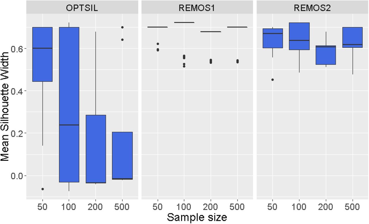
Increasing sample size seriously decreased the performance of OPTSIL in terms of both optimization success and time efficiency (Fig. 5., Fig. 6.). With 50 points, median MSW was near 0.6, than it dropped to 0.24 at 100 points. Surprisingly, with 200 and 500 points the median MSW was below 0 which means very high number of misclassified objects in the final solution. Notably, MSW varied very broadly at all sample sizes with OPTSIL. With REMOS1 median MSW was near 0.7 in all cases with minimal variation. REMOS2 produced somewhat lower MSW medians (between 0.6 and 0.7) and higher variation. Runtimes increased with sample size in case of all three methods but, again, they differed regarding the slope of this relationship and the range of runtimes. OPTSIL reached the final solutions within 1 s with 50 points; however, with 500 points it needed approximately 1000 s. REMOS1 was approximately 10 times faster: with 50 points it performed similarly but with the largest sample it took approximately 100 s. The fastest was REMOS2 which reached final solutions within 0.1 s with the smallest sample and approximately 1 s with the largest.

The change of mean silhouette width along increasing sample size for the three optimization methods in case of the artificial data set

The change of runtime along increasing sample size for the three optimization methods in case of the artificial data set
Discussion
All of our tests showed that REMOS algorithms are equivalent or, more often, superior to OPTSIL both in terms of optimization and time efficiency. The very high runtime demand of OPTSIL is mentioned by Roberts (2015). In terms of optimization efficiency, OPTSIL performed better than REMOS algorithms in only one case: with the Grassland data set and two clusters. The low MSWs obtained by OPTSIL are surprising given that OPTSIL directly optimizes on this criterion, while REMOS algorithms do not. As Roberts (2015) stated, OPTSIL optimization always flows towards the steepest decline in MSW. As a consequence, OPTSIL can easily converge into a local optimum and cannot proceed towards a farther optimum. Thus, if initiated from different classifications of the same data set, OPTSIL solutions can vary considerably.
In contrast, REMOS algorithms do not directly optimize MSW but they minimize the number of objects which decrease MSW, thus they increase MSW indirectly. Our results show that this approach can lead to higher final MSW and faster optimization. Additionally, REMOS algorithms provided less variable final classifications in terms of MSW. REMOS1 performed the best in terms of optimization success, while REMOS2 was outstandingly fast. Hence, re-assigning the worst classified objects one-by-one, as it is done in REMOS1, seems an efficient way to find a high final MSW. Moderate time efficiency of REMOS1 can be its weakness in case of very large data sets, many clusters, and noisy initial classification. Despite its on-average lower final MSW values, REMOS2 might be a useful alternative in such cases, due to its short runtime. An important property of REMOS2 is that if there is a cluster in the initial classification which comprises only points with silhouette widths below the threshold (by default, below 0), all of them will be re-assigned to their neighbour cluster, respectively, thus the number of clusters can be lower in the optimized classification than in the initial one. This is advantageous when the optimal number of clusters is not known. In such a case, a classification with more clusters than expected as optimal should be used for initiating REMOS2, which is able cancel weakly defined clusters during the optimization.
Conclusions
We present REMOS1 and REMOS2 as new reallocation methods for the optimization of classifications. Both methods performed better than the recently introduced OPTSIL, both in optimization efficiency and runtime. REMOS1 reached higher final mean silhouette widths, while REMOS2 were superior regarding computation time.
Abbreviations
- MSW
- mean silhouette width
- PAM
- partitioning around medoids


