

Abstract
The Theory of Island Biogeography (TIB) promoted the idea that species richness within sites should depend on site connectivity, i.e. its connection with surrounding potential sources of immigrants. TIB has been extended to a wide array of fragmented ecosystems, beyond archipelagoes, surfing on the analogy between habitat patches and islands and the patch-matrix framework. However, patch connectivity often little contributes to explaining species richness in empirical studies. Before interpreting this trend as questioning the broad applicability of TIB principles, one first needs a clear identification of methods and contexts where strong effects of patch structural connectivity are likely to occur. Here, we use spatially explicit simulations of neutral metacommunities to show that patch connectivity effect on local species richness is maximized under a set of specific conditions: (i) patch delineation should be fine enough to prevent dispersal limitation within patches, (ii) patch connectivity indices should be scaled according to target organisms’ dispersal abilities and (iii) habitat amount and fragmentation should both lie in some intermediary range that still needs an empirically tractable definition. When those three criteria are met, the absence of effect of connectivity on species richness should be interpreted as contradicting TIB principles.
Introduction
Since the Theory of Island Biogeography (TIB) [1], it is commonly acknowledged that species presence within local community depends on their ability to immigrate, and that geographic isolation of communities can negatively affect species richness. TIB principles have been extended to a wide array of ecosystems beyond archipelagoes (see [2,3] for reviews and critical appraisal), leading to studying how the availability of suitable habitat nearby can act as a source of immigrants and affect species richness within local communities. Such generalization of TIB relied on adopting a “patch-matrix” description of habitat in space, where one decomposes the map of some suitable habitat into patches that correspond to potential communities (analogous to islands in an archipelago), the rest of space being considered unhospitable for species.
The geographic isolation of patches has been developed into the concept of “patch structural connectivity”, which quantifies the potential exchanges of immigrants between a focal patch and the surrounding habitats [4]. Most of the indices that aim at quantifying patch structural connectivity consist in counting patches around the focal patch, using weights proportional to patch area (or quality) and decreasing with distance to the focal patch. For instance, the “distance to nearest neighbor” index gives weight 1 to the closest patch and 0 for others. Buffer indices give positive weights to patches closer to the focal patch than some threshold distance, and weight 0 to patches outside this range. More generally, indices based on a distance kernel give to patches weights that decrease with distance to the focal patch according to some pre-defined kernel function (e.g. [5]).
In a meta-analysis of 1’015 empirical studies on terrestrial systems covering a broad taxonomical range and spread at global scale, [6] evidenced that patch structural connectivity measured as distance to the nearest patch tend to have weak predictive power on species presence within patches (median deviance explained equaled c.a. 20%). This study brings some evidence showing that the limited success of patch connectivity indices may come from: inadequate use of structural connectivity indices based on surrounding habitat rather than functional connectivity indices based on surrounding populations, inadequate delineation of patches for species harboring multiple life stages with contrasted requirements and overlooking the type of matrix surrounding the habitat patch, hence questioning the validity of the patch-matrix framework for terrestrial systems.
Questioning the validity of the TIB or the patch-matrix framework for terrestrial systems or arguing for the use of functional rather than structural patch connectivity indices are sound criticism of current practices. However, the TIB framework based on structural connectivity is has the strong advantage of being quite simple and straightforward to implement in a broad array of empirical systems. Before discarding it for more involved methodologies, one should make sure that its limited success in past studies does not come from methodological limitations that can be fixed. For instance, another review of 122 empirical studies [7], which covered terrestrial and aquatic systems and analyzed the presence or abundance of 954 species, evidenced that effects of local environmental conditions within a patch on species presence or abundance occurred more frequently (71% of species analyses) than the effects of patch structural connectivity (55% of species analyses). These authors mentioned methodological limits as a major explanation of the limited success of patch structural connectivity indices: the lack of statistical power, i.e. insufficient number of patches and the inadequate patch structural connectivity metrics, buffer indices being more performant than widely used isolation metrics. Here we argue that a critical appraisal of the TIB framework needs identifying first which methods for measuring patch structural connectivity and which properties of the habitat spatial distribution of studied systems are expected to yield strong effects of patch structural connectivity on local species richness. If the TIB framework fails when both methods and context are expected to be adequate then the conceptual ground of the approach can be undoubtedly questioned.
The lack of strong effects of patch structural connectivity indices on local species richness may come from the fact that the patch structural connectivity indices used in empirical studies do not efficiently capture the immigration intensity. For instance, [8,9] showed that indices based on the distance to the nearest patches are poor predictors of species presence compared indices based on a distance kernel, like buffers. [9] further showed that even when complementing distance to nearest patches with the area of the focal patch, buffer were still better predictor of species richness. This tend to suggest that patch connectivity indices can intrinsically differ in their ability to capture the contribution of immigration to species richness within a focal patch. Here, we aimed at comparing how three types of patch connectivity indices coming from contrasted frameworks differed or not in their explanatory power of species richness.
Among indices based on a distance kernel, the tuning of “scaling parameters” (i.e. parameters driving the speed of patch weight decrease with distance) with respect to target organisms dispersal also modulates the explanatory power of patch connectivity indices. Using simulations of a metacommunity on patch networks, [10] showed that changing the scaling of patch connectivity indices (i.e. how fast patch weights decrease with distance) can change the effect size of connectivity on species Simpson diversity. They further showed that the higher the dispersal ability of species, the larger the scaling of indices should be to reach the best possible explanatory power. Similarly, a metapopulation simulation study [11] showed that there exists some optimal buffer radius that maximizes the effect size of connectivity upon local presence of a target species. They further suggested that this optimal size, called the “scale of effect” should lie between four and nine times the average dispersal distance of the target species. Therefore, choosing an appropriate scaling of patch connectivity indices with respect to typical dispersal distances of target organisms should improve the ability of patch connectivity indices to capture a negative effect of geographic isolation on species richness. Here, we aimed at testing whether the scaling of patch connectivity indices that maximizes the explanatory power upon species richness increased with dispersal distance of target organisms, as suggested by previous findings.
Patch definition and delineation must adapt to the questions and patterns under study [12]. For instance, in studies about foraging strategies, defining a patch according to the perceptual range of target organisms can be adequate. By contrast, in the context of the TIB, patches should correspond to discrete areas of habitat within which individuals from multiple species have access and compete for all the resource without space limitation over their lifetime, hence making relevant entities for community-scale studies. [12] extensively developed how focusing on inappropriate patch scale in optimal foraging could lead to unexpected patterns. Similarly, [13] showed in a simulation study that the negative relationship between species richness and distance to mainland in the classic TIB may collapse when applied to entire archipelagoes rather that single islands, because of internal limited dispersal. Therefore, a decisive step in the analysis of patch connectivity effects on local species richness is therefore to convert the raw raster of habitat pixels into patches of appropriate size. Often, the delineation of patches follows a “vector map” perspective, according to [14] terminology : set of contiguous pixels corresponding to “habitat” are lumped together to form polygons denoted as patches. However, this approach brings no guarantee that emerging patches have the appropriate size to constitute potential communities for target organisms. In particular, when habitat is little fragmented, it creates large patches and subsequent connectivity indices potentially miss a large part of connectivity effects, which may take place within patches. Such mismatch may weaken the link between patch-based connectivity and community features measured from a local sample. We propose that building patches from a “raster” perspective (still following [14] terminology), using a grid with mesh size smaller or equal to the average dispersal distance of target organisms should ensure the appropriate patch delineation for the study and contribute to increase the explanatory power of patch connectivity indices on species richness. In particular, large contiguous sets of habitat pixels should be split to obtain patches of adequate dimension. Here, we aimed at comparing the performance of patch connectivity indices computed from a vector map perspective to those obtained from a raster perspective with mesh size adapted to the dispersal distance of target organisms. We expected that using a raster with mesh size smaller or equal to the dispersal distance of target organisms would greatly improve the performance of indices.
Patch connectivity indices with appropriate scaling used in on patches with adequate delineation can still yield limited effects on local species richness. This occurs for instance if structural connectivity little fluctuates among patches or if immigration does not act as a source of species diversity. Limited fluctuation in patch connectivity indices arises when most patches have similar surrounding habitat availability. For a given quantity of habitat in a landscape, we anticipated that the variance of surrounding habitat availability among patches increased with habitat aggregation. Here, we therefore aimed at testing whether, habitat amount being kept constant, a stronger aggregation of the habitat map would lead to stronger fluctuation of patch connectivity indices, hence creating opportunities to observe connectivity effects on local species richness.
Furthermore, even if patch structural connectivity adequately depicts immigration and varies among patches, it can affect local species richness only if the immigrant pool coming to the focal patch harbors a moderate-to-high species diversity. The immigrant pool is made of a mixture of emigrants from patches in the surrounding landscape. Consequently, the diversity of the immigrant pool is tightly linked to the concept of γ-diversity [15] of the surrounding landscape (i.e. mixing all patches together). For a given amount of surrounding habitat (controlled by patch connectivity indices), the gamma diversity of the surrounding landscape depends on the spatial configuration of the habitat, although the relationship can be labile. If the surrounding habitat has high landscape connectivity in the absence of the focal patch, it may increase the local species diversity in each patch contributing to the immigrant pool (α-diversity in the surrounding landscape; e.g. [16]). However, it may also decrease the dissimilarity in species composition among contributing patches (β-diversity in the surrounding landscape; e.g. [16]), resulting in uncertain global effect on the γ-diversity. Nonetheless, a robust conclusion is that the spatial configuration of the surrounding habitat is likely to generate “noise” on the patch connectivity – species richness relationship, and such noise may contribute to weaken the explanatory power of patch connectivity indices on species richness. Patch-based “connector” indices [17] can contribute to pinpoint fluctuation in landscape connectivity around the focal patch. These indices capture to what extent the focal patch contributes to the connection among the other patches in the landscape. For a given amount of habitat around the focal patch, a lower connector score of the focal patch therefore indicates that surrounding patches depend less on the focal patch to connect one with another, i.e. that direct fluxes among surrounding patches are stronger. Here we aimed at testing whether the explanatory power of patch connectivity indices on the local species richness decreased when the connector status of sampled patches have strong independent fluctuations, which we called “connector noise”. Because [18] showed that connector indices are often decoupled from patch connectivity indices in space, this situation was likely to occur in our simulations and in the real world, hence worth considering here.
In our analysis, we successively focused on how patch delineation, scaling of patch connectivity indices, index type and landscape features (including variation of patch connectivity index and connector noise) affect the explanatory power of patch structural connectivity on local species richness. We used a virtual ecologist approach [19] relying on metacommunity simulations in a spatially-explicit model. Virtual datasets stemming from such models constituted an ideal context to assess the impact of our factors of interest, for they offered perfect control of the spatial distribution of habitat and the ecological features of species. In particular, they only included processes related to the TIB (immigration, ecological drift; [20]), thus maximizing our ability to study how methodological choices and landscape features affect the explanatory power of patch structural connectivity. We anticipated that explanatory powers generated by this approach would necessarily be an over-estimation of what occurs in real ecosystems, where many processes unrelated to TIB may be at work. However, feedbacks from our virtual approach to real ecosystems readily arise when considering that settings that negatively affects the explanatory power of patch structural connectivity in our approach have very little chance to yield strong explanatory power of patch structural connectivity on local species richness in empirical studies.
Materials and methods
Landscape generation
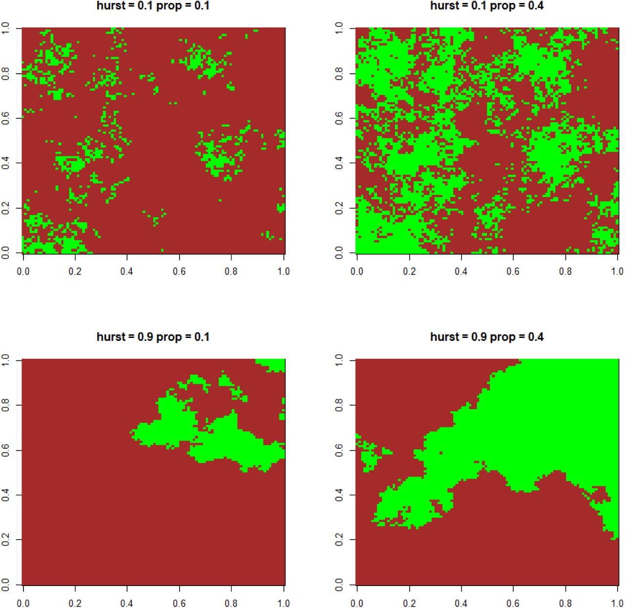
We considered binary landscapes made of suitable habitat cells and inhospitable matrix cells. We generated virtual landscapes composed of 100×100 cells using a midpoint-displacement algorithm [21] which allowed us covering different levels of habitat quantity and fragmentation. The proportion of habitat cells varied according to three modalities (10%, 20% of 40% of the landscapes). The spatial aggregation of habitat cells varied independently, and was controlled by the Hurst exponent (0.1, 0.5, and 0.9 in increasing order of aggregation; see Fig. S1 for examples). Ten replicates for each of these nine landscape types were generated, resulting in 90 landscapes. Higher values of the Hurst exponent for a given value of habitat proportion increased the size of sets of contiguous cells and decreased the number of distinct sets of contiguous cells (Fig. S2). Higher habitat proportion for a constant Hurst coefficient value also resulted in higher mean size of sets of contiguous cells.

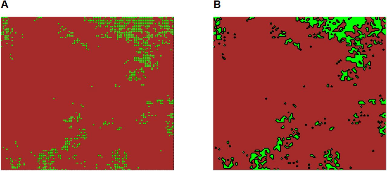
Habitat is pictured in green, matrix in brown.

Colors correspond to distinct combinations of Hurst exponent and habitat proportion. Ellipses correspond to 95%-CI of a fitted bivariate Student distribution.
Neutral metacommunity simulations
We simulated spatially explicit neutral metacommunities on virtual heterogeneous landscapes. We resorted to using a spatially explicit neutral model of metacommunities, where all species have the same dispersal distance. We used a discrete-time model where the metacommunity changes by steps. All habitat cells were occupied, and community dynamics in each habitat cell followed a zero-sum game, so that habitat cells always harbored 100 individuals at the beginning of a step. One step was made of two consecutive events. Event 1: 10% of individuals die in each cell – they are picked at random. Event 2: dead individuals are replaced by the same number of recruited individuals that are randomly drawn from a multinomial distribution, each species having a weight equal to 0.01×χi + ∑k Aik exp(-dkf /λs) where χi is the relative abundance of species i in the regional pool, Aik is the local abundance of species i in habitat cell k, dkf is the Euclidean distance (in cell unit) between the focal habitat cell f and the source habitat cell k, λs is a parameter defining species dispersal distances and the sum is over all habitat cells k of the landscape. The regional pool was an infinite pool of migrants representing biodiversity at larger spatial scales than the focal landscape, it contained 100 species, the relative abundances of which were sampled once for all at the beginning of the simulation in a Dirichlet distribution with concentration parameters αi equal to 1 (with i from 1 to 100). Metacommunity were simulated forward in time, with 1000 burn-in steps and 500 steps between each replicates. Simulation was structured as a torus to remove unwanted border effects in metacommunity dynamics. Metacommunities were simulated with three levels of species dispersal λs = 0.25, 0.5, 1 cell, which corresponded to median dispersal distance of 0.6, 0.7, 0.9 cell and average dispersal distance of 0.6, 0.8,1.2 cells. Because dispersal distance distribution is skewed, it is also insightful to give the 95% quantile of dispersal distance, which corresponded to 1.2, 1.7, 3.1 cells respectively, and shows the potential of species in terms of long-distance dispersal. We performed 10 replicates for each dispersal value and in each landscape. In total, we obtained of 3 Hurst coefficient values × 3 habitat proportion × 3 species dispersal level × 10 landscape replicates × 10 community replicates = 2700 metacommunity simulations. For each metacommunity simulation, species richness was computed at the cell level with R [22].
Finally, we built one virtual dataset per simulation. We considered communities in habitat cells away from each other’s for a minimal distance of 12 cells, to reduce spatial auto-correlation (e.g. Fig. 1A). We also reduced potential landscape border effect (that could decouple landscape indices and actual migrants received) by excluding cells near landscape borders (to a distance inferior or equal to eight cells, equivalent to the longest buffer radius). Each landscape counted in average 25 sampled cells (CI-95% = [23, 27]).

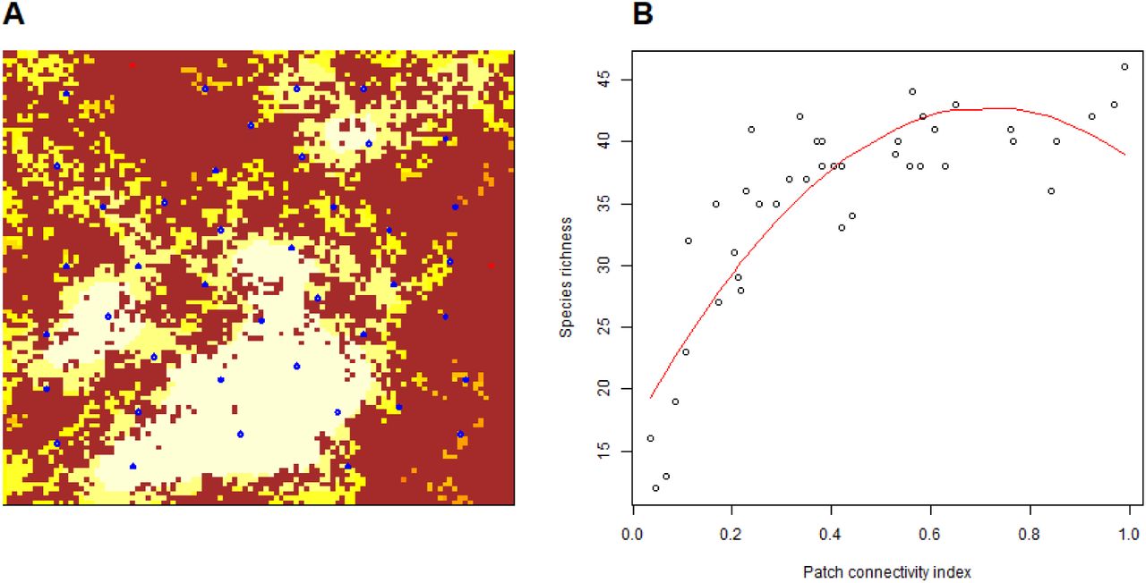
Panel A: a virtual landscape obtained through midpoint displacement algorithm, with controlled habitat proportion (here 0.4) and Hurst coefficient (here 0.1). Brown cells stands for unhospitable matrix. Red to yellow cells denote habitat cells with increasing patch connectivity indices (here a Buffer index with radius 8 cells). Sampled cells are selected (blue circles) with minimal distance from border and among cells. We simulated metacommunity dynamics in the whole landscape. At the end of simulation, species richness is recorded in sampled cells. Panel B: the relationship between patch connectivity and sampled cells is analysed using a quadratic model (red curve), and the R2 of the model, called R2spec, is recorded for future analyses. When not significant, the quadratic term is dropped. The community dispersal in the simulation presented here is λs = 1 cell.
Local connectivity indices
We first computed patch connectivity indices using a raster perspective for patch delineation, considering each habitat cell in the landscape as a patch. We called this approach “fine” patch delineation below. In the context of our simulation, it is the appropriate patch delineation to consider, since habitat cells correspond to communities in the metacommunity model. We computed three contrasted types of patch connectivity indices (Table 1) for each sampled cell of virtual datasets: Buffer, dF and dIICflux. Buffer indices correspond to the proportion of area covered by habitat patches within circles of different radius (rbuf = 1, 2, 4, 5, 8 cells) around the focal sampled patch. dIICflux and dF were based on nodes corresponding to patches. Pairs of nodes were connected to each other by links. Links’ weights wij between cells i and j in the network decreased according to the formula exp(-dij/λc), where dij is the Euclidean distances between cells i and j and λc is a scale parameter [14,23]. λc may be interpreted as the hypothesized scale of dispersal distance of target organisms in the landscape (which may differ from the “true” simulated scale of dispersal distance, which is λs). We considered four scale parameter values (λc = 0.25, 0.5, 1 and 2 cells). dF quantified the sum of edges weights between the focal patch (i.e. the sampled cell) and all the other patches (i.e. all the other habitat cells of the landscape). dIICflux considered a binary graph, where each cell pair was considered either connected (1) or not (0) relatively to a minimal link weight wmin = 0.005. Scale parameters λc = 0.25, 0.5, 1 and 2 cells thus lead to connect all pairs of habitat cells separated by a distance inferior to 1.3, 2.6, 5.3 and 10.6 cells respectively. In particular, binary graph for λc = 0.25 hence corresponded to the classic stepping-stone on a grid. dIICflux captured a notion of node centrality, like dF, but based on topological distance in the graph rather than Euclidean distance. All indices were computed with Conefor 2.7 (command line version for Linux, furnished by S. Saura, soon publicly available on www.conefor.org; [24]).
Then, we switched to a vector perspective in patch delineation, lumping together the groups of contiguous habitat cells in the map to form patches (Fig. S3), which we call a “coarse” patch delineation below. For each sampled cells, we computed the connectivity of the patch it belonged to. With this coarse patch delineation, patches contained several communities connected by limited dispersal. Altogether, we computed 28 distinct patch connectivity indices in each sampled cell of each simulation.
Panel A shows a habitat map where fine delineation of patches has been applied. Panel B shows the same habitat map where coarse patch delineation has been applied, i.e. sets of contiguous cells has been lumped together. Contiguity is based on the Von Neuman neighborhood of cells.
General statistical approach
We analyzed the explanatory power of patch connectivity indices on local species richness in simulated datasets. The explanatory power of a patch connectivity index on species richness is defined as the R2 coefficient of the model Species richness ∼ Patch connectivity + (Patch connectivity)2, where we dropped the quadratic term when not significant (e.g. Fig. 1B). We denoted these R2 coefficients as “R2spec” below. Most of our analyses consisted in analyzing how patch delineation, index scaling and landscape features affect R2spec, using linear models with R2spec as a dependent variable.
Patch delineation
We first considered dF and dIICflux patch connectivity indices computed with a fine patch delineation. In each of the 2700 simulated dataset, we recorded R2spec for dF or dIICflux. Both dF and dIICflux had 4 possible scaling values, potentially yielding four distinct R2spec values per index for the same virtual dataset. However, we only kept the best value out of four in our analysis of patch delineation. We thus obtained 2’700 datasets × 2 indices = 5’400 R2spec values.
Then we considered patch connectivity indices computed with a coarse patch delineation. In each of the 2700 simulated dataset, we fitted a linear model with species richness as a dependent variable. We used the connectivity index (dF or dIICflux) and the area of the patch containing the sampled cell as independent variables. We included patch area in the analysis to ensure fair comparison with the fine patch delineation analysis. Here again we included quadratic terms (dF2 or dIICflux2, and area2) when significant. We recorded R2spec of the models and kept only the highest values across possible scaling parameters, which yielded again 2’700 × 2 = 5’400 R2spec values.
We then analyzed the 10800 R2spec values generated above with one linear model per index type (dF or dIICflux), where the dependent variable R2spec was modelled as a function of the patch delineation (“coarse” or “fine”) in interaction with landscape Hurst coefficient, landscape habitat proportion and species dispersal distance (all these dependent variables being considered as factors). We expected R2spec to be significantly higher at fine patch delineation (despite the fact that area is included in the analysis at coarse patch delineation), which we tested using the model R2spec∼resolution. We also expected the positive effect of switching from coarse to fine resolution to increase when Hurst coefficient or habitat proportion increase, because sets of contiguous cells become larger on average, leading to stronger limited dispersal effects within patches. We tested this second hypothesis using two models with interactions: R2spec∼resolution × Hurst coefficient and R2spec∼resolution × habitat proportion. At last, we expected the positive effect of switching from coarse to fine patch delineation to decrease when species dispersal increases, because limited dispersal within sets of contiguous cells weakens. We tested this last hypothesis using the model: R2spec∼resolution × dispersal.
Index scaling – We then considered Buffer, dIICflux and dF patch connectivity indices computed with a fine patch delineation. In each of the 2700 simulated dataset, we recorded R2spec for each patch connectivity index and each scaling parameter value. We thus obtained 2’700 datasets × 3 indices × 4 or 5 scaling parameter values = 35’100 R2spec values. We then built one linear model per index type (Buffer, dF or dIICflux), where R2spec was the dependent variable, modelled as a function of species dispersal distance in interaction with index scale parameter R2spec ∼ dispersal × scaling value. We expected that the scale parameter yielding the highest R2spec values increase with the dispersal distance of species, following previously published results in the literature.
Landscape features
For each patch connectivity index type and each virtual dataset, we considered a fine patch delineation and selected the scaling parameter value (within the explored range) that maximized R2spec. We recorded this maximal value of R2spec, hence generating 2700 virtual datasets × 3 index types = 8100 R2 values.
We explored separately for each index at each species dispersal level how landscape features (i.e. the habitat proportion and the Hurst coefficient) affected R2spec using the linear model R2 ∼ Hurst coefficient × habitat proportion. We expected that landscapes the highest Hurst coefficient value yield highest R2spec.
We finally explored whether additional landscape features, beyond Hurst coefficient and habitat proportion, could bring additional explanatory power on the variation of the R2spec with optimal scaling and resolution among virtual datasets. We focused on Buffer index and considered two additional landscape features.
For each of the 2700 virtual datasets, we computed the standard deviation of Buffer among sampled cells (“Buffer s.d.”) and the explanatory power of Buffer over sampled cells’ connector value (“Connector R2”). We defined Connector R2 as the R2 coefficient of the model connector value ∼ Buffer + Buffer2. We used dIICconnector [17] as a connector value. Like dIICflux presented above, dIICconnector is an index based on representing the habitat map as a binary network of patch (recall that at fine resolution patches are cells). To obtain the binary network, we used the same weighting procedure than for dF and dIICflux, and chose a scaling parameter λc = 2 cells (the largest value considered in our study). We used the same threshold on edges weight than above (wmin = 0.005) to decide whether patches should be connected or not in the binary graph. We defined our two additional landscape features of interest as the residual variation of Buffer s.d. and Connector R2 with respect to Hurst coefficient and habitat proportion. We computed them as the residuals of linear models Buffer s.d. ∼ Hurst coefficient × habitat proportion and Connector R2 ∼ Hurst coefficient × habitat proportion respectively (we applied one linear model per dispersal level).
For each species dispersal level, we fitted the model R2spec ∼ Hurst coefficient × habitat proportion + residual Buffer s.d. + residual connector R2 over the 900 virtual datasets. We expected that residual Buffer s.d. have a significant positive effect on R2spec. We also predicted that residual connector R2 have a significant positive effect on R2spec. We assessed the relative contribution of Hurst coefficient × habitat proportion, residual Buffer s.d. and residual connector R2 using an analysis of variance.
Results
Patch delineation
For both dF and dIICflux, using a fine patch delineation yielded higher R2spec on average than using a coarse resolution (+0.18 with p<2e-16 for dF; +0.07 with p<2e-16 for dIICflux).
For dF index, the Hurst coefficient did not significantly affect the positive effect of refining patch delineation on R2spec. By contrast, a larger proportion of habitat in the landscape increased the positive effect of refining patch delineation on R2spec (Fig. 2A): the effect of refining patch delineation on R2spec reached +0.23 (estimate s.d. 0.01) for a habitat proportion of 0.4 while it equaled +0.14 (estimate s.d. 0.01) only for a habitat proportion of 0.1. Higher species dispersal decreased the positive effect of refining patch delineation on R2spec (Fig. 2B): the effect of refining patch delineation on R2spec reached +0.27 (estimate s.d. 0.01) when species had low dispersal abilities while it equaled +0.06 (estimate s.d. 0.01) when species had high dispersal abilities.

Bars show the average R2spec over simulated datasets for distinct levels of habitat proportion (panel A), community dispersal (panel B) and Hurst coefficient (panel C), with asymptotic 95% confidence intervals (half width = 1.96 x standard error). Panel A and B come from the analysis of the dF index while Panel C comes from the analysis of dIICflux, hence the different colors.
For dIICflux index, a higher Hurst coefficient increased the positive effect of refining patch delineation on R2spec (Fig. 2C): the effect of refining patch delineation equaled +0.10 (estimate s.d. 0.01) in highly aggregated landscapes with a Hurst coefficient of 0.9 while the effect of refining patch delineation equaled +0.05 only (estimate s.d. 0.01) in landscapes with a Hurst coefficient of 0.1. Habitat proportion and species dispersal did not significantly affect the effect of refining patch delineation on R2spec.
Index scaling and species dispersal
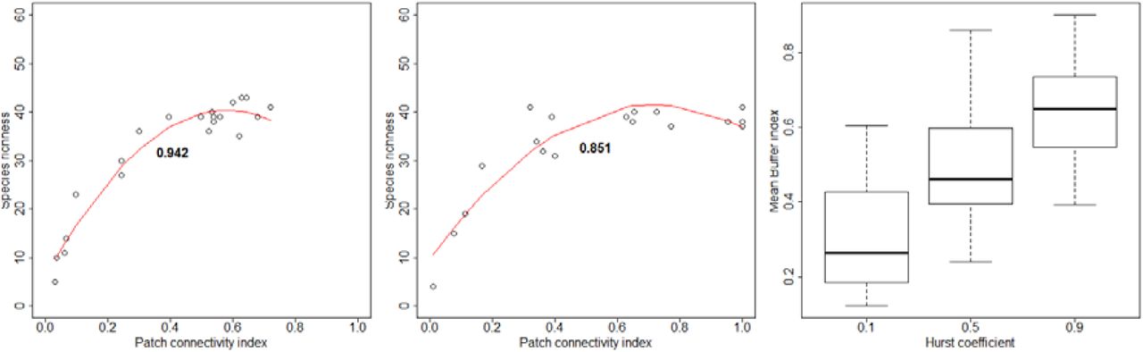
For Buffer, dF and dIICflux, the scaling parameter value yielding the highest R2spec increased with species dispersal (Fig. 3).

Panels A, B and C correspond to Buffer, dF and dIICflux indices respectively. Shapes correspond to the distinct community dispersal levels tested in our analysis. The y-axis corresponds to the average R2 observed across our virtual datasets for the target index when using the scaling parameter value reported on the x-axis. Error bars correspond to asymptotic 95% confidence intervals (half width = 1.96 x standard error).
For Buffer indices, the optimal scaling parameter value (i.e. Buffer radius rbuf) corresponded to about 8 times the true scale of species dispersal (λs; Fig. 3A). For dF indices, the optimal scaling parameter (λc) corresponded to about 2 times the true scale of species dispersal (Fig. 3B). For dIICflux indices, the optimal scaling parameter (λc) rather corresponded to about 0.5 times the true scale of species dispersal (Fig. 3C; although the scope of scaling parameters explored was not sufficient to ascertain this point for all the three dispersal levels explored).
For all species dispersal levels and all indices, R2spec varied broadly (by about 0.2) when browsing possible scaling values. However, the optimal scaling value rarely yielded R2spec markedly different from those obtained from neighboring scaling values, except in some specific cases were the optimal value lied at the boarder of the explored range (suggesting that the true optimal scaling value is actually outside the explored range; see e.g. dIICflux with species dispersal 0.25 on Fig. 3C).
Global performance of indices
95% of R2spec values at fine patch delineation with optimal scaling lied between 0.30 and 0.96, with an average value of 0.74. Buffer and dF stood out as the most performant index on average. The average R2spec of Buffer was R2spec=0.78. Average R2spec for dF index differed from Buffer by -0.01 only, which was a significant (z-test; p=0.03) but very weak difference. By contrast, the average R2spec for dIICflux index differed from Buffer by -0.12, which was a more significant (z-test; p<2e-16) and stronger difference.
Landscape effects
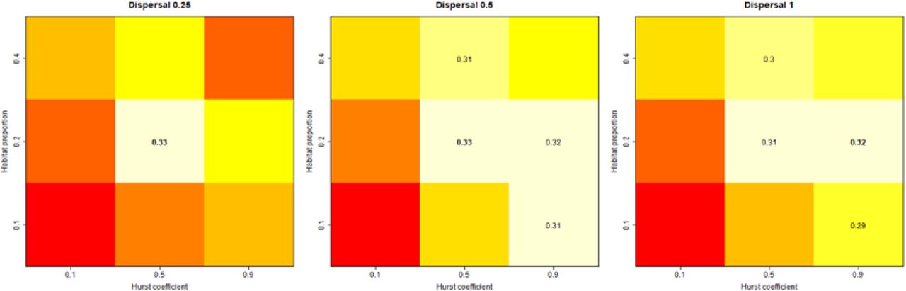
R2spec of patch connectivity indices were generally maximized for landscapes combining intermediary levels of the Hurst coefficient and intermediary levels of habitat proportion, irrespective of species dispersal (Fig. 4). The only exception occurred for dIICflux with medium or high species dispersal level, where landscapes with low habitat proportion and high aggregation yielded the highest R2spec.

Each panel corresponds to one index type applied to virtual datasets with one species dispersal level (i.e. 900 virtual datasets). Columns correspond to dispersal levels (in cell unit), and lines to index type. Within a panel, average R2spec is reported for each combination of habitat proportion (y-axis) and Hurst coefficient (x-axis). Within a panel, the heat map shows the ordination of R2spec values with red corresponding to lowest values and white to highest ones. The maximum R2spec value is reported in bold letters, and all the other R2spec that are not significantly different from the maximum based on a z-test with threshold 5% are also reported.
For Buffer index, the variation in Hurst coefficient and habitat proportion among virtual datasets explained between 97% and 99% of the variance in R2spec (Fig. 5). Residual Buffer s. d. had a significant positive on R2spec, with standardized effect size (i.e. after scaling residual Buffer s. d.) equal to 0.05 (estimate s.d. = 0.004), 0.05 (estimate s.d. = 0.002) and 0.06 (estimate s.d. = 0.004) for low, intermediate and high species dispersal respectively. The effect of residual Buffer s.d. was therefore significant but consistently low and explained a very limited amount of R2spec variance (around 0.5%; Fig. 5). The residual Connector R2 had a significant positive effect on R2spec at high species dispersal level only, but the magnitude of the contribution was then negligible (Fig. 5).

Variance is decomposed into the contributions of: (i) the variation in landscape features (Hurst coefficient in interaction with habitat proportion); (ii) the variation of Buffer standard deviation among landscapes of similar features (“Buffer s.d.”); (iii) the variation in the explanatory power of Buffer on the connector index in sampled cells among landscapes of similar features (“Connector R2”). Contributions (y-axes) are expressed in percentages of the total variance of R2spec. Panel A shows the whole decomposition. Panel B shows all the contributions except that of landscape features, for better readability.
Discussion
Patch delineation
We have illustrated the problem of patch delineation in a binary design comparing outputs of considering each elementary cell as a patch (the appropriate resolution with respect to simulations) versus considering sets of contiguous cells as patches. Effects of patch connectivity indices on local species richness were higher at fine patch delineation, where no dispersal limitation occurred within patches. The coarser patch delineation considering sets of contiguous habitat as patches led to important drop of explanatory power in our results, reaching about -0.2 when species harbored strong dispersal limitation (Fig. 2B). In the light of our results, we therefore champion the “raster” perspective of [14]: even when target habitats form “intuitive” patches (e.g. forest patches in agricultural landscapes), one should define a priori a grid with appropriate mesh size, equal or lower to the scale of dispersal for target organisms and use it to decompose the habitat map in elementary units. We also insist on the fact that the raster perspective is perfectly compatible with the use of graph theory concepts among cells, as we illustrated with the use of indices such as dIICflux or dIICconnector on fine patch delineation.
Determining a priori the appropriate mesh size is not an easy task, especially since in real communities – contrary to our simulations - movement capacity and dispersal are heterogeneous among species. Beyond the binary comparison between coarse and fine patch delineation that we proposed here, one should now explore the sensitivity of patch connectivity indices explanatory power to varying mesh size (as suggested by [25] in real empirical studies) This would allow assessing whether some degree of uncertainty on that parameter is acceptable. We anticipate that using a too fine patch delineation should not lead to heavy loss of explanatory power of patch connectivity indices on species richness, as long as patch connectivity indices are rescaled appropriately. For instance, in our study design, the range of probable dispersal distances (95% quantile) is closer to mesh size for low species dispersal (1.2 cells) than for high species dispersal (3.1 cells). When species dispersal is high, one could therefore argue that mesh size is unnecessarily small. However, we did not observe important drops of power of patch connectivity indices when moving from low to high species dispersal (e.g. Fig. 4). If using too fine a mesh size is harmless, mesh size should thus be adjusted on the limiting species in terms of movement capacity in communities with heterogeneous movement and dispersal, i.e. those that are the less mobile in space and interact with other organisms only at fine scale. This approach should probably be preferred to approaches based e.g. on the average movement capacity across species of the community.
However, choosing very fine patch delineation can be computationally challenging, since it can increase by several orders of magnitude the number of spatial units. This particularly affect indices stemming from graph theory that needs to determine shortest paths between all pairs of spatial units. Here we have been able to compute dIICflux and dIICconnector indices in all the virtual landscapes at fine resolution (up to 4000 habitat units in a single landscape). Consequently, indices based on binary networks seem to pass the test of computational time. By contrast, we were unable to compute analogous indices in weighted networks (dPCflux and dPCconnector; [26]).
Index scaling
The scaling of patch connectivity indices leading to maximal explanatory power on species richness (the “scale of effect” sensu [11]) increased with the dispersal distance of target organism, in line with previous findings on virtual studies [10,11]. This is a strong argument to prefer patch connectivity indices with a scaling parameter that can be modulated to match the dispersal ability of organisms rather that indices that cannot be adapted like distance to nearest patch. It also confirms that the scale of effect should capture some quantitative features of species dispersal, as it is often contended in the empirical literature (e.g. [27,28]).
However, the scale of effect should not be used as a quantitative estimate of dispersal distance for two reasons. First, we observed that scaling parameter values around the optimal one often generated a very small loss of explanatory power, suggesting that the explanatory power was not highly sensitive to errors on scaling parameter value. Therefore, finding the scaling parameter that maximizes the correlation is probably not an accurate method to obtain estimate of species dispersal level. This is consistent with the fact that, in empirical systems, buffer radii maximizing the explanatory power over species presence or abundance can spread over a large array of distances without significant drop of explanatory power, sometimes covering several orders of magnitude (e.g. [29]). Second, the quantitative relationship between the scale of effect and species dispersal was labile. We identified linear relationships between the scale of effect and the scale of species dispersal used in simulations (λs), but the slope was very different depending on the index used. In addition, no analogous linear relationships arose when considering average, median or 95% quantile of species dispersal, contrary to what was evidenced by [11] on abundance in a virtual metapopulation study.
Therefore, the relationship between the scale of effect and the scale of species dispersal distance can contribute to ranking dispersal distance among species or groups of species with marked differences. It can also contribute, when some a priori information is available about the dispersal distance of target organisms, to defining the range of scaling parameter values in which the scale of effect should be searched for.
Here we considered neutral metacommunities where all the species have the same dispersal distance. This greatly simplified the analysis of the relationship between the scale of effect of indices and species dispersal distances. However, species dispersal distances in real communities are known to be heterogeneous [30,31], as polymorphism on dispersal is a strong driver of species coexistence at metacommunity scale [32,33]. On may therefore question how our findings can transfer to real empirical studies. We already commented earlier that for a given species dispersal distance a quite broad range of scaling parameters for a given index can lead to levels of explanatory power similar to that of the scale of effect. While we presented this pattern as an obstacle to species dispersal estimation, it could turn out to be an advantage when species have heterogeneous species dispersal strategy. As a matter of fact, a scaling parameter value adapted to the average dispersal distance of species in the community might be fairly adapted to all the species in the community. Of course, this should not be valid anymore if species dispersal is highly heterogeneous among species.
Global performance of indices
Indices used with appropriate scaling and fine spatial resolution yielded very high explanatory power values on species richness, way above what usually occurs in empirical studies. We expected that result, which stems from the fact that our simulations only include processes compatible TIB, i.e. limited dispersal and ecological drift, and force species dispersal to be equal. By doing so, it creates ideal conditions for high explanatory power of patch connectivity on species richness to occur and offers us magnifying glasses to focus on how patch delineation, indices properties and landscape features can modulate it. Any downward effects on the explanatory power in our approach could result in a total disappearance of patch connectivity explanatory power in real studies, and should therefore be interpreted as bad conditions to study patch connectivity contribution in empirical systems.
Buffer and dF indices lead to high and very similar performance when used with appropriate scaling. This stemmed from the fact that these two indices are highly correlated (average correlation across landscapes above 0.95; Figure S4). In our study, Buffer resembled dF index when the buffer radius was about 4 times the dF scaling parameter value. [8] had already evidenced that correlations between IFM index (a generalization of the dF index; [34]) and buffers could reach 0.9 in a real landscape (their study did not focus on how the scaling of both indices could affect the correlation). Such a similarity between Buffer and dF on patches with fine delineation was quite expected since both indices share the same general structure: a weighted sum of surrounding habitat cells contribution where weights decreases with Euclidean distance following some kernel function. Regarding the shape of the kernel, Buffer is based on a step function while dF is based on an decreasing exponential kernel. We therefore interpret our results as the fact that changing the decreasing function used as a kernel may little affect the local connectivity as long as scaling is adjusted. This may explain why [5] found that: (i) switching from buffer to continuously decreasing kernel little affected AIC or pseudo-R2 of models used to predict species abundances; (ii) neither continuously decreasing nor step function was uniformly better to explain species abundance across four case studies; (iii) different continuous shapes of kernel had quite indiscernible predictive performance.

We presented correlations among Buffer, dF and dIICflux using ascending hierarchical classification. Within each of the 90 simulated landscapes, we computed the values of the 13 indices (accounting for distinct scaling values) in all habitat cells, which yielded 13 vectors of length 1000 to 4000 depending on the habitat proportion. We scaled each of the 13 vectors to mean 0 and variance 1, divided them by the square root of the number of habitat cells in the landscapes and computed pairwise Euclidean distances among them. We thus obtained one 13×13 distance matrix among patch connectivity indices in each of the 90 landscapes. Note that the distance between two indices corresponds to  , where r is the Pearson correlation between the indices across all habitat cells of the considered landscapes. We then averaged the 90 distance matrices to obtain one single 13×13 distance matrix as a basis for classification. We ran an ascending non-supervised classification (hclust function of R base package), using the complete method for group merging. A monophyletic group G with common ancestor located at value r means that any pair of indices within G has a correlation above r. Indices labels in the dendrogram are made of three parts separated by underscores “_”. The first part of the name indicates the type of the index (“buf”, “dF”, “dIICflux”). The second part of the name indicates the scale parameter of the index (“d025”, “d050”, “d100”, “d200” corresponding to λc = 0.25, 0.5, 1, 2 cells respectively, and “1”, “2”, “4”, “6”, “8” corresponding to buffer radius rbuf in cells). The last part in meaningless here.
The dIICflux index had a lower explanatory power than Buffer and dF indices on average (−0.12 on Rspec). This difference in global performance was made possible by the fact that dIICflux harbored a different profile than dF and Buffer in landscapes (Fig. S4), because it considers topological rather than Euclidean distance to compute connectivity. The use of five scaling values only in our analysis calls for some caution in the interpretation dIICflux lower explanatory power. The optimal scaling value of dIICflux for low and intermediate dispersal seemed to lie below the lower limit of the range explored in our study. Consequently the explanatory power of this index might be underestimated compared to the other ones and partly explain why it seems less efficient in predicting species richness.
Part of the relative success of dF and Buffer over dIICflux may also stem from the fact that we did not include different resistance values to habitat and matrix cells. When heterogeneous resistance occurs, landscape connectivity including displacement costs (e.g. least cost path, circuit theory) can be markedly different from prediction based on Euclidean distance only [35], and may better capture the movement of organisms in real case study [36,37]. This probably also applies to patch connectivity. By connecting only cells that contain habitat, dIICflux and other indices based on topological distance within a graph could prove more performant when matrix has high resistance cost, and we may not find the same superiority of Euclidean indices as in our simulations. However, some of our results here should remain true when resistance is heterogeneous in space, at least qualitatively. Indeed, since our study is purely virtual, we could as well consider that distances among cells in the habitat map are not Euclidean but ecological distances. This would have amounted to saying that landscapes considered in our study are “distorted” maps compared to reality. Based on this mind experiment, we would still expect that the optimal scaling of indices, expressed in ecological distance, would increase with species dispersal, expressed in ecological distance too. We also expect that our conclusion about the adequate delineation of patches should also hold, but the mesh size in the real map should then fluctuate in space depending on the resistance cost, shrinking in habitat areas with high resistance and expanding in habitat areas with low resistance cost.
Landscape effects
Landscapes combining intermediary levels of the Hurst coefficient and intermediary levels of habitat proportion yielded highest explanatory of dF and Buffer indices used with adapted scaling at fine spatial resolution. We understood the unpredicted unimodal effect of habitat proportion on the explanatory power as follows: high connectivity is unlikely in landscapes with a very low amount of habitats while low connectivity is unlikely in landscapes with a very low amount of habitats. As a result, the maximal range of variation in patch connectivity lies in intermediary landscapes in terms of habitat proportion (Figure S5). Our findings are reminiscent of the conceptual model of [38], which promoted the idea that habitat spatial configuration should affect species abundance or persistence only in when habitat amount lies in a intermediary range of values. The latter range is comprised between a lower limit where the species cannot maintain in the landscape whatever the spatial configuration and an upper limit where the species can maintain in the landscape whatever the spatial configuration. Whether and how the levels of habitat proportion at which, one the one hand, patch connectivity – local species richness relationship arises and, on the other hand, species persistence is sensitive to landscape-scale configuration overlap is an open question of practical interest. In particular, one may ask whether the presence of a patch connectivity – local species richness could indicate that the habitat amount at landscape scale has entered the intermediary range where considering the spatial configuration in management plans becomes critical.

Each panel corresponds to one species dispersal level (i.e. 900 virtual datasets). Within a panel, average standard deviation of Buffer index among sampled cells is reported for each combination of habitat proportion (y-axis) and Hurst coefficient (x-axis). Within a panel, the heat map shows the ordination of standard deviation values with red corresponding to lowest values and white to highest ones. The maximum average standard deviation value is reported in bold letters, and all the other values that are not significantly different from the maximum based on a z-test with threshold 5% are also reported.
Contrary to what we predicted, the Hurst coefficient had a modal effect on the explanatory power of dF and Buffer on species richness. The increasing part of the relationship actually followed the predicted behavior: low aggregation creates landscapes where the habitat is homogeneously spread in space, leading to low variance in patch connectivity among sampled cells (Fig. S5), hence low explanatory power on species richness. Landscape with high aggregations contained few distinct sets of large contiguous cells (Fig. S1, S2). The variance in patch-connectivity of cells thus depended on the ratio between the distance to the border of these sets and the scaling parameter of the patch connectivity index. When dispersal was low, variation in patch connectivity could occur only in a thin stripe along the border of the sets of contiguous cells, the rest of cells harboring a uniformly high, saturating connectivity. There was therefore little opportunity for low connectivity, hence creating low variance of patch connectivity indices (Fig. S5) leading to low explanatory value of indices on species richness (Fig. 4). By contrast, when dispersal is medium or high, there was a smoother contrast between border and interior of patches in term of connectivity, yielding more opportunity for variance in patch connectivity and no negative effect of Hurst coefficient on patch connectivity variance (Fig. S5). However, the effect size Buffer indices on species richness still became smaller when switching from medium to high Hurst coefficient because the average value of Buffer index increased and the variation in Buffer then fell within a range of values where the corresponding species richness tended to saturate at an upper threshold (Fig. S6). Given the tight level of correlation between Buffer and dF, our conclusions about Buffer can be harmlessly transferred to dF index.
In all panels, the species dispersal is λs=1, the highest value explored in our study. Buffer index has a radius rbuf= 8 cells which is the optimal scaling given λs. Left panel: an example of fit of the model species richness ∼ Buffer + Buffer2 for intermediary habitat proportion and intermediary Hurst coefficient. The coefficient of determination Rspec is reported in bold. Center panel: an example of fit of the model species richness ∼ Buffer + Buffer2 for intermediary habitat proportion and high Hurst coefficient. The coefficient of determination Rspec is reported in bold. Right panel: boxplot of average Buffer value across sampled cells as a function of Hurst coefficient. The thick horizontal line shows the median value, boxes delimit first and third quantiles, and whiskers encompass all the data.
The variance in Buffer index among landscapes with identical Hurst coefficient and habitat proportion had an additional positive effect on its explanatory power, as expected, but this effect was clearly negligible compared to landscape influence. We had the same type of conclusion regarding the potential perturbation induced by fluctuation in the connector status of patches independently from their connectivity. We only detected a weak negative effect of connector noise (the contrary of Connector R2) on the explanatory power of patch connectivity indices at high species dispersal.
Conclusion
Our results suggest that finding a strong effect of patch structural connectivity on local species richness can occur only if: (i) spatial units used as patches are sufficiently small to prevent internal dispersal limitation within patches, which can be obtained by using a raster perspective with appropriate mesh size for patch delineation; (ii) the scaling of the patch connectivity index is adapted to the dispersal ability of species considered, which can be obtained by browsing scaling parameters over a range of values defined from a priori knowledge about species dispersal distance; (iii) the studied landscape shows intermediate habitat amount and intermediate habitat fragmentation, so that the patch connectivity index can harbor high variance among sampled patches. Notwithstanding the success of Buffer in our approach, we suggest that similar analyses as ours should be performed with heterogeneous resistance cost before recommending kernel-based indices using Euclidean distance upon other choices. To date, point (iii) seems less straightforward to use in empirical studies because it is not clear a priori what should be an “intermediate” habitat amount or fragmentation and a “sufficient” level of variance in patch connectivity index for some target set of species. It probably depends on species dispersal but maybe also on the spatial extent of the study. Further work, dedicated to this point, is now needed in order to define a full set of empirically verifiable conditions necessary for observing connectivity effects on local species richness.
Conflict of interest disclosure
The authors of this preprint declare that they have no financial conflict of interest with the content of this article. FL and FJ belong to the panel of PCI Ecology recommenders.
Acknowledgments
We thank Santiago Saura for sharing CONEFOR code. This work was part of the Patrames project funded by the convention 2016 n°2101870336 of the French Ministry of Environment (Water and Biodiversity Direction).
Footnotes
Thanks to the time and effort that PCI Ecology recommanders and reviewers spent reading and commenting our manuscript. We have fully revised it in the light of their remarks. (1) We refocused the manuscript on our main question (when should connectivity drive species richness) and streamlined the whole text accordingly. (2) We dropped unclear references to the habitat amount hypothesis, which would deserve another study. (3) We used quadratic relationships to study connectivity effects. (4) We dropped the combination of indices of various types, since a single index already led to very high R2 with the quadratic regression, making combination of indices prone to spurious effects. (5) We strengthened the use of bibliographical references.
References


