

Abstract
This work considers a class of biologically plausible cost functions for neural networks, where the same cost function is minimised by both neural activity and plasticity. In brief, we show that such cost functions can be cast as a variational bound on model evidence, or marginal likelihood, under an implicit generative model. Using generative models based on Markov decision processes (MDP), we show, analytically, that neural activity and plasticity perform Bayesian inference and learning, respectively, by maximising model evidence. Using mathematical and numerical analyses, we then confirm that biologically plausible cost functions—used in neural networks—correspond to variational free energy under some prior beliefs about the prevalence of latent states generating inputs. These prior beliefs are determined by particular constants (i.e., thresholds) that define the cost function. This means that the Bayes optimal encoding of latent or hidden states is achieved when, and only when, the network’s implicit priors match the process generating inputs. Our results suggest that when a neural network minimises its cost function, it is implicitly minimising variational free energy under optimal or sub-optimal prior beliefs. This insight is potentially important because it suggests that any free parameter of a neural network’s cost function can itself be optimised—by minimisation with respect to variational free energy.
Introduction
Cost functions are used to solve problems in various scientific fields—including physics, chemistry, engineering and machine learning. Furthermore, any optimisation problem that can be specified using a cost function can be formulated as a gradient descent; enabling one to treat neuronal dynamics and plasticity as an optimisation process. Neuroscience commonly uses cost functions to express various types of learning: for instance, supervised learning to minimise the differences between outputs and targets, as in a perceptron (Marr, 1969; Albus, 1971); reinforcement learning to maximise future reward (Schultz et al., 1997; Sutton & Barto, 1998), and unsupervised learning to maximise the efficiency of encoding (Linsker, 1988; Brown et al., 2001). These examples highlight the importance of specifying a problem or function in terms of cost functions, from which neural and synaptic dynamics can be derived. In other words, cost functions offer a formal (i.e., normative) expression of the purpose of a neural network and prescribe the dynamics of that neural network. Crucially, once the cost function has been established, it is no longer necessary to consider the dynamics. We can, instead, characterise the neural network’s behaviour in terms of fixed points, transients, attractors and structural stability—based on and only on the cost function. In short, it is important to identify the cost function for a neural network to understand its dynamics, plasticity, and function.
A ubiquitous cost function in neurobiology, theoretical biology, and machine learning is model evidence, or equivalently, marginal likelihood or surprise; namely, the probability of some input or data under a model of how those inputs were generated by unknown or hidden causes. Generally, the evaluation of surprise is intractable. However, this evaluation can be converted into an optimisation problem by inducing a variational bound on surprise. In machine learning, this is known as an evidence lower bound (ELBO), while the same quantity is known as variational free energy in statistical physics and theoretical neurobiology.
Variational free energy minimisation is a candidate principle governing neuronal activity and synaptic plasticity (Friston et al., 2006; Friston, 2010). Here, surprise reflects the improbability of sensory inputs, given a model of how those inputs were caused. In turn, minimising variational free energy, as a proxy for surprise, corresponds to inferring the (unobservable) causes of (observable) consequences. To the extent that biological systems minimise variational free energy, it is possible to say that they infer the hidden states that generate their sensory inputs (Helmholtz, 1925; Knill & Pouget, 2004; DiCarlo et al., 2012) and consequently predict those inputs (Rao & Ballard, 1999; Friston, 2005). This is generally referred to as perceptual inference based upon an internal generative model about the external world (Dayan et al., 1995; George & Hawkins, 2009; Bastos et al., 2012).
Variational free energy minimisation provides a unified mathematical formulation of these inference and learning processes in terms of self-organising neural networks that function as Bayes optimal encoders. Moreover, organisms can use the same cost function to control their surrounding environment by sampling predicted (i.e., preferred) inputs. This is known as active inference (Friston et al., 2011). The ensuing free-energy principle suggests that active inference and learning are mediated by changes in neural activity, synaptic strengths, and the behaviour of an organism to minimise variational free energy, as a proxy for surprise. Crucially, variational free energy and model evidence rest upon a generative model of continuous or discrete hidden states. A number of recent studies have used Markov decision process (MDP) generative models to elaborate schemes that minimise variational free energy (Friston, FitzGerald et al., 2016; Friston, FitzGerald et al., 2017; Friston, Parr et al., 2017). This minimisation reproduces various interesting dynamics and behaviours of real neuronal networks and biological organisms. However, it remains to be established whether variational free energy minimisation is an apt explanation for any given neural network, as opposed to optimisation of alternative cost functions.
In principle, any neural network that produces an output or a decision can be regarded as performing some form of inference in terms of Bayesian decision theory. On this reading, the complete class theorem suggests that any neural network could be regarded as performing Bayesian inference under some prior beliefs; therefore, it could be regarded as minimising variational free energy. The complete class theorem (Wald, 1947; Brown, 1981) says that for any pair of decisions and cost functions, there are some prior beliefs (implicit in the generative model) that render the decisions Bayes optimal. This suggests that it should be theoretically possible to identify an implicit generative model within any neural network architecture, which renders its cost function a variational free energy or ELBO. In what follows, we show that such an identification is possible for a fairly canonical form of neural network and a generic form of generative model.
In brief, we adopt a reverse engineering approach to identify a plausible cost function for neural networks—and show that the resulting cost function is formally equivalent to variational free energy. For simplicity, we focus on blind source separation (BSS); namely the problem of separating sensory inputs into multiple hidden sources or causes (Belouchrani et al., 1997; Cichocki et al., 2009; Comon & Jutten, 2010), which provides the minimum setup for modelling causal inference. We have previously observed BSS performed by in vitro neural networks (Isomura et al., 2015) and have reproduced this self-supervised process using an MDP and variational free energy minimisation (Isomura & Friston, 2018). These works suggest that variational free energy minimisation offers a plausible account of empirical behaviour of in vitro networks.
In this work, we ask whether variational free energy minimisation can account for the normative behaviour of any neural network, by considering all possible cost functions (i.e., possible purposes). Using mathematical analysis, we identify a class of cost functions—from which update rules for both neural activity and synaptic plasticity can be derived—when a single-layer feed-forward neural network comprises firing rate neurons with sigmoid activation. The gradient descent on the ensuing cost function leads naturally to Hebbian plasticity with an activity-dependent homeostatic term. We show that these cost functions are formally homologous to variational free energy, under an MDP. Finally, we discuss the implications of this result for explaining the empirical behaviour of neuronal networks, in terms of free energy minimisation under particular prior beliefs.
Methods
In this section, we first derive the form of a variational free energy cost function under a specific generative model; namely a Markov decision process1. We will go through the derivations carefully, with a focus on the form of the ensuing Bayesian belief updating. The form of this updating will re-emerge later, when reverse engineering the cost functions implicit in neural networks. This section starts with a description of Markov decision processes—as a general kind of generative model—and then considers the minimisation of variational free energy under these models.
Generative models
Under an MDP scheme (Fig. 1A), a minimal BSS setup—in a discrete-space—can be expressed as the likelihood mapping (A) from N hidden sources or states st ≡ st1 ⊗ … ⊗stN to M observations ot ≡ ot1⊗ …⊗otM (using the outer product operator ⨂). Each source and observation take one (ON state) or zero (OFF state) values for each time step (stk ∈ {0,1}, oti ∈ {0,1}). Throughout this manuscript, k indices the k-th hidden state, while i indices the i-th observation. The probability of st follows a categorical distribution P(st) = P(st1) … P(stN) = Cat(D1) … Cat(DN), where Dk ≡ (Dk1, Dk0) with Dk1 + Dk0 = 1.

Comparison between an MDP scheme and a neural network. (A) MDP scheme expressed as a Forney factor graph (Forney, 2001; Dauwels, 2007) based upon the formulation in (Friston, Parr et al., 2017). In this BSS setup, the prior D determines hidden states st and st determines observation ot through the likelihood mapping A. Inference corresponds to the inversion of this generative process. Here D∗ indicates the true prior while D indicates the prior that the network operates under. If D = D∗, inference would be optimal and biased otherwise. (B) Neural network comprising a single layer feed-forward network with a sigmoid activation function. The network receives sensory inputs yt = (yt1, …, ytM) that are generated from hidden states st = (st1, …, stN) and outputs neural activities xt = (xt1, …, xtN). Here, yti corresponds to a binary outcome oti, and xtk should encode the posterior expectation about a binary state stk.
The probability of an outcome is determined by the likelihood mapping, from hidden states to observations, in terms of a categorical distribution A: P(oti|st, Ai) = Cat(Ai), where the elements of Ai are given by  . This determines the probability of oti takes j ∈ {0,1} when st = (l1, …, lN). The prior distribution of Ai is defined by Dirichlet distribution P(Ai) = Dir(ai) with sufficient statistics (concentration parameter) ai. We use õ ≡ (o1, …, ot) to denote a sequence of observations and
  a sequence of hidden states. Formally, the generative model (i.e., the joint distribution over outcomes, hidden states and the parameters of their likelihood mapping) is expressed as

Minimisation of variational free energy
In this MDP scheme, the aim is to minimise surprise or, equivalently, maximise marginal likelihood by minimising variational free energy; i.e., performing approximate or variational Bayesian inference. From the generative model, we can motivate a mean-field approximation to the posterior (recognition) density as follows
 where the marginal posterior distributions of st and A are categorical Q(sτ) = Cat(sτ) and Dirichlet Q(Ai) = Dir(aτ) distributions, respectively. Note that sτ and ai denote sufficient statistics (i.e., sτ gives expectations between zero and one, and ai expresses the concentration parameter). Below, we use the posterior expectation of ln Ai to encode posterior beliefs about the likelihood, which is given by
 using the digamma function ψ(⋅). Here
  denotes the expectation over Q(Ai). The variational free energy of this generative model is then given by:
 where 𝒟KL[⋅ || ⋅] is complexity as scored by the Kullback-Leibler divergence (Kullback & Leibler, 1951) and ℬ(ai) ≡ Γ(ai1)Γ(ai0)/Γ(ai1 + ai0) is the beta function. The first term in the final equality comprises accuracy and the state complexity, which increases in proportion to time t. Conversely, the second term—the complexity of parameters—increases in the order of ln t and is thus negligible when t is large (see Supplementary Methods S1 for details). In what follows, we will therefore drop parameter complexity, under the assumption that the scheme has experienced a sufficient number of outcomes.
Inference optimises posterior expectations about the hidden states by minimising variational free energy. The optimal posterior expectations are obtained by solving the variation of F to give:
 where σ(⋅) is the softmax function. As stk is a binary value in this study, the posterior expectation of stk taking a value of one (ON state) can be expressed as
 using the sigmoid function sig(z) ≡ 1/(1 + exp(−z)). (The posterior expectation of stk taking a value 0 (OFF state) is thus stk0 = 1 − stk1.) Here, Dk1 and Dk0 are constants denoting the prior beliefs about hidden states. Bayes optimal encoding is obtained when, and only when, the prior beliefs match the genuine prior distribution; i.e., Dk1 = Dk0 = 0.5 in this BSS setup. This concludes our treatment of inference about hidden states under this minimal scheme. Note that the updates in Equation (5) have a biological plausibility in the sense that the expectations can be associated with nonnegative firing rates, while the arguments of the sigmoid (softmax) function can be associated with neuronal depolarisation; rendering the softmax function a voltage-firing rate activation function
In terms of learning, the optimal posterior expectations about the parameters are given by:
 where ai is the prior, ⨂ expresses the operator of outer product, and
  . Thus, the optimal posterior expectation of matrix A is A⋅⋅k = a⋅⋅k/(a⋅1k + a⋅0k), or equivalently
 where
where  ,
,  , and
, and  . Whereas,
  and
and  . Here
  is a vector of ones. The prior of parameters ai is in the order of 1 and thus negligible when t is large. The four vectors (A⋅1k1, A⋅1k0, A⋅;0k1, A⋅0k0) express the optimal posterior expectations of ot taking ON state when stk is ON (A⋅1k1) or OFF (A⋅1k0), or ot taking OFF state when stk is ON (A⋅0k1) or OFF (A⋅0k0). Although this expression may look complicated, it is fairly straightforward: the posterior expectations of the likelihood simply accumulate posterior expectations about the co-occurrence of states and their outcomes. These accumulated (Dirichlet) parameters are then normalised to give a likelihood or probability. Crucially, one can see the associative or Hebbian aspect of this belief updating; expressed here in terms of the outer products between (presynaptic) expectations about states and (postsynaptic) outcomes in Equation (7). We now turn to the equivalent updating for activities and parameters or weights of a neural network.
Neural activity and Hebbian plasticity models
Next, we consider the neural activity and synaptic plasticity in the neural network (Fig. 1B). We will assume that the k-th neuron’s activity xtk is given by
 where yt ≡ (yt1, …, ytM)T = (ot11, …, otM1)T is a column vector of inputs that encodes the ON states of ot. We suppose Wk1 ∈ ℝM and Wk0 ∈ ℝM comprise row vectors of synapses, and hk1 ∈ ℝ and hk0 ∈ ℝ are adaptive thresholds that depend on the values of Wk1 and Wk0, respectively. One may think Wk1 and Wk0 express excitatory and inhibitory synapses, respectively. We will further assume that the nonlinear leakage f′(⋅) is the inverse of the sigmoid function, such that the fixed point of xtk is given by

We further assume that synaptic strengths are updated following Hebbian plasticity, with an activity-dependent homeostatic term, as follows:
 where Hebb1 and Hebb0 mediate Hebbian plasticity as determined by the product of sensory inputs and neural outputs, and Home1 and Home0 are homeostatic plasticity determined by output neural activity.
In the MDP scheme, posterior expectations about hidden states and parameters are usually associated with neural activity and synaptic strengths. Here, we can see a formal similarity between the solutions for expectations about states (Equation (6)) and activity in the neural network (Equation (10)). By this analogy, xtk can be regarded as encoding the posterior expectation of the ON state sτk1, and Wk1 and Wk0 correspond to  and
and  , respectively; in the sense that they express the amplitude of yt = ot⋅1 influencing xtk.
The optimal posterior expectation of a hidden state taking a value of one (Equation (6)) is given by the ratio of the beliefs about ON and OFF states, expressed as a sigmoid function. Thus, to be a Bayes optimal encoder, the fixed point of neural activity needs to be a sigmoid function. This is assured when f′(xτk) is the inverse of the sigmoid function (see Equation (13) below). Under this condition the fixed point or solution for xtk is given by Equation (10), which compares inputs from ON and OFF pathways. This means xtk encodes the posterior expectation of the k-th hidden state being ON—that is, xtk → stk1. In short, the neural network is effectively inferring the hidden state.
If the activity of the neural network is performing inference, does the Hebbian plasticity correspond to Bayes optimal learning? In other words, does the synaptic update rule in Equation (11) ensure neural activity and synaptic strengths asymptotically encode Bayesian optimal posterior beliefs about hidden states (xtk → stk1) and parameters (Wk1 → sig−1(A⋅1k1)), respectively? To address this, we will identify a class of cost functions from which the neural activity and synaptic plasticity can be derived and consider the conditions under which the cost function becomes consistent with variational free energy.
Neural network cost functions
Here, we consider a class of functions that constitute a cost function for both neural activity and synaptic plasticity. We start by assuming that the update of k-th neuron’s activity (Equation (9)) is determined by the gradient of cost function Lk,  . By integrating the right-hand side of Equation (9), we obtain a class of cost functions as
 where 𝒪(1) depends on Wk1 and Wk0 that is of smaller order than 𝒪(t) and thus negligible when t is large. The cost function of the entire network is defined by
  . When f′(xτk) is the inverse of the sigmoid function, we have
 up to a constant term. We further assume that the synaptic weight update rule is derived from the same cost function Lk. Thus, the synaptic plasticity is given by
 where
where  ,
,  ,
,  ,
,  ,
,  , and
, and  . Note that the update of Wk1 is not directly influenced by Wk0, and vice versa; since they encode parameters in physically distinct pathways (i.e., the updates are local learning rules (Lee et al., 2000)). The update rule for Wk1 can be viewed as Hebbian plasticity mediated by an additional activity-dependent term expressing homeostatic plasticity. Moreover, the update of Wk0 can be viewed as anti-Hebbian plasticity with a homeostatic term, in the sense that Wk0 is reduced when input (yt) and output (xtk) fire together. The fixed points of Wk1 and Wk0 are given by

Crucially, these synaptic strength updates are a subclass of the general synaptic plasticity rule in Equation (11); see also Supplementary Methods S2 for mathematical explanation. Therefore, if the synaptic update rule is derived from the cost function that underwrites neural activity, the synaptic update rule has a biologically plausible form, comprising Hebbian plasticity and activity-dependent homeostatic plasticity.
Comparison with variational free energy
Here, we establish a formal relationship between the cost function L and variational free energy. We define Vk1 ≡ sig(Wk1) and Vk0 ≡ sig(Wk0) as nonlinear functions of synaptic strengths. We consider the case where neural activity is expressed as a sigmoid function and thus Equation (13) holds. From  , Equation (12) becomes

One can immediately see a formal correspondence between this cost function and variational free energy (Equation (4)). That is, when we assume xtk = stk1, Vk1 = A⋅1k1, and Vk0 = A⋅1k0, Equation (16) has exactly the same form as the sum of the accuracy and state complexity (see the first term in the last equality of Equation (4)), which is the leading order term of variational free energy.
Specifically, when the threshold  and
and  .
.  hold, Equation (16) becomes equivalent to Equation (4) up to the ln t order term (that disappears when t is large). Therefore, in this special case, the fixed points of neural activity and synaptic strengths become posterior expectations; thus, xtk asymptotically becomes the Bayes optimal encoder for a large t limit (provided Dk matches the genuine prior
  ).
).
We can define  and
and  as functions of Wk1 and Wk0, respectively, and express the cost function as

Here, we suppose—without loss of generality—that the constant terms in ϕk1 and ϕk0 are chosen to ensure exp(ϕk1) + exp(ϕk0) = 1. Under this condition, (exp(ϕk1), exp(ϕk0)) can be viewed as the prior belief about hidden states
 and thus Equation (17) is equivalent to the accuracy and state complexity terms of variational free energy.
In other words, when the prior belief about states (Dk1, Dk0) is a function of the posterior expectation about parameters (A⋅1k1, A⋅1k0), the generic cost function under consideration can be expressed in the form of variational free energy, up to 𝒪(ln t) term. A generic cost function L is sub-optimal from the perspective of Bayesian inference unless ϕk1 and ϕk0 are tuned appropriately to express the unbiased (i.e., optimal) prior belief. In this BSS setup, ϕk1 = ϕk0 = const is optimal; thus, a generic L would asymptotically give an upper bound of variational free energy with the optimal prior belief about states when t is large.
Analysis on synaptic update rules
For the purpose of explicitly solving the fixed point of Wk1 and Wk0 that provide the global minimum of L, we suppose ϕk1 and ϕk0 as linear functions of Wk1 and Wk0, respectively, given as
 where αk1, αk0 ∈ ℝ and βk1, βk0 ∈ ℝM are constants. By solving the variation of L with respect to Wk1 and Wk0, we find the fixed point of synaptic strengths as

Since the update from t to t+1 is expressed as sig(Wk1 + ΔWk1) − sig(Wk1) = sig(Wk1)(1 − sig(Wk1))ΔWk1 + 𝒪(|ΔWk12|) and sig(Wk1 + ΔWk1) − sig(Wk1) ≈  , we recover the following synaptic plasticity:
 where ⊙ denotes the element-wise (Hadamard) product and sig(Wk1)⊙−1 indicates the element-wise inverse of sig(Wk1). This synaptic plasticity rule is a subclass of the generic synaptic plasticity rule in Equation (11).
In summary, under a few minimal assumptions and ignoring small contributions to weight updates, the neural network under consideration can be regarded as minimising an approximation to model evidence or marginal likelihood because the cost function can be formulated in terms of variational free energy. In what follows, we will rehearse these analytic results and then use numerical analyses to illustrate Bayes optimal inference (and learning) in a neural network when, and only when, it has the right priors.
Results
Analytical form of neural network cost functions
The analysis of the preceding section rests on the following assumptions:
(1) Updates of neural activity and synaptic weights are determined by a gradient descent on a cost function L.
(2) Neural activity is updated by the weighted sum of sensory inputs and its fixed point is expressed as the sigmoid function.
Under these assumptions, we can express the cost function for a neural network as follows (see Equation (17)):
 where Vk1 = sig(Wk1) and Vk0 = sig(Wk0) hold, and ϕk1 and ϕk0 are functions of Wk1 and Wk0, respectively. The log likelihood function (accuracy term) and divergence of hidden states (complexity term) of variational free energy emerge naturally under the assumption of a sigmoid activation function. The cost function above has additional terms denoted by ϕk1 and ϕk0. In other words, we can say that the cost function L is variational free energy under a sub-optimal prior belief about hidden states—depends on Wk1 and Wk0: ln P(stk) = ln Dk = ϕk, where ϕk ≡ (ϕk1, ϕk0). This prior alters the landscape of cost function in a sub-optimal manner and thus provides a biased solution for neural activities and synaptic strengths, which differ from the Bayes optimal encoders.
For analytical tractability, we further assume the following:
(3) The perturbation terms (ϕk1 and ϕk0) that constitute the difference between cost function and variational free energy with optimal prior beliefs can be expressed as linear equations of Wk1 and Wk0.
From assumption 3, Equation (17) becomes:
 where {αk1, αk0, βk1, βk0} are constants. The cost function has degrees of freedom with respect to the choice of constants {αk1, αk0, βk1, βk0}, which correspond to the prior belief about states Dk. The neural activity and synaptic strengths that give the minimum of a generic physiological cost function L are biased by these constants, which may be analogous to physiological constraints.
The fixed point of synaptic strengths—that give the minimum of L—is given analytically as Equation (20), expressing that (βk1, βk0) deviates the centre of the nonlinear mapping—from Hebbian products to synaptic strengths—from the optimal position (shown in Equation (8)). As shown in Equation (14), the derivative of L with respect to Wk1 and Wk0 recovers the synaptic update rules that comprise Hebbian and activity-dependent homeostatic terms. Although Equation (14) expresses the dynamics of synaptic strengths that converge to the fixed point, it is consistent with a plasticity rule that gives the synaptic change from t to t+1 (Equation (21)).
Hence, based on assumptions 1 and 2, we find that the cost function approximates variational free energy: see also Supplementary Table S1 for their correspondence. Under this condition, neural activity encodes the posterior expectation about hidden states: xτk = sτk1 = Q(sτk = 1) and synaptic strengths encode the posterior expectation of the parameters: Vk1 = sig(Wk1) = A⋅1k1 and Vk0 = sig(Wk0) = A⋅1k0. In addition, based on assumption 3, the accuracy of approximation depends on the deviation of constants {αk1, αk0, βk1, βk0} from their optimal values. From a Bayesian perspective, these constants can be viewed as prior beliefs, ln P(stk) = ln Dk = (αk1+ Wk1βk1, αk0 + Wk0βk0), when we assume (xk, 1 − xk) represents the state posterior stk. When and only when (αk1, αk0) = (− ln 2, − ln 2) and  , does the cost function becomes variational free energy with optimal prior beliefs (for BSS), whose global minimum ensures Bayes optimal encoding.
In short, we identify a class of biologically plausible cost functions from which the update rules for both neural activity and synaptic plasticity can be derived. When the activation function for neural activity is a sigmoid function, a cost function in this class is expressed straightforwardly as variational free energy. With respect to the choice of constants expressing physiological constraints in the neural network, the cost function has degrees of freedom that—from the Bayesian perspective—may be viewed as (potentially sub-optimal) prior beliefs. We now illustrate the implicit inference and learning in neural networks, using simulations of BSS.
Numerical simulations
Here, we simulate the dynamics of neural activity and synaptic strengths when they perform a gradient descent on the cost function in Equation (22). We consider a BSS comprising two hidden sources (or states) and 32 observations (or sensory inputs), formulated as an MDP. The two hidden sources comprise four patterns: st1 ⨂ st2 = (0,0), (1,0), (0,1), (1,1). An observation oti is generated through the likelihood mapping Ai. We defined Ai with:

Here, for example, Ai110 = 3/4 for 1 ≤ i ≤ 16 is the probability of oti taking one when st = (1,0). The simulations continue over T = 104 time steps.
First, we show that—as in (Isomura & Friston, 2018)—a network with a cost function with optimised constants ((αk1, αk0) = (− ln 2, − ln 2) and  performs BSS successfully (Fig. 2). The responses of neuron 1 came to recognise source 1 after training, indicating that neuron 1 learnt to encode source 1 (Fig. 2A). Conversely, neuron 2 learnt to infer source 2 (Fig. 2B). This demonstrates that minimisation of the cost function, with optimal constants, is equivalent to variational free energy minimisation—and is sufficient to emulate BSS. Next, we quantified the dependency of BSS performance on the form of the cost function, by varying the above constants (Fig. 3).

Emergence of response selectivity for a source. (A) Evolution of neuron 1’s responses that learnt to encode source 1, in the sense that the response is high when source 1 takes a value of one (red dots), and it is low when source 1 takes a value of zero (blue dots). Lines correspond to smoothed trajectories obtained using a discrete cosine transform. (B) Emergence of neuron 2’s response that learnt to encode source 2. Codes are appended as Supplementary Source Codes.

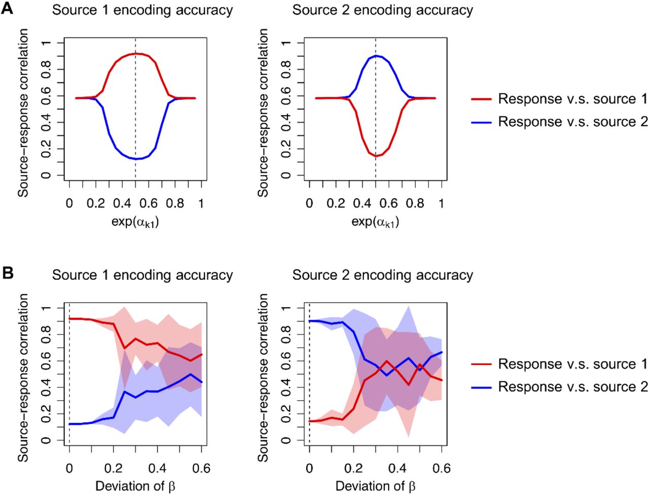
Dependence of source encoding accuracy on constants. Left panels show the magnitudes of correlations between sources and response of a neuron expected to encode source 1: |corr(st1, xt1)| and |corr(st2, xt1)|. The right panels show the magnitudes of the correlations between sources and response of a neuron expected to encode source 2: |corr(st1, xt2)| and |corr(st2, xt2)|. (A) Dependence on the constant α that controls the excitability of a neuron, when β is fixed to zero. The dashed line (0.5) indicates the optimal value of exp(αk1). (B) Dependence on constant β, when α is fixed as (αk1, αk0) = (− ln 2, − ln 2). Elements of β were randomly generated from a Gaussian distribution with zero mean. The standard deviation of β was varied (horizontal axis), where zero deviation was optimal (dashed line). Lines and shaded areas indicate the mean and standard deviation of the source-response correlation, evaluated with 10 different values of β. Codes are appended as Supplementary Source Codes.
We found that changing (αk1, αk0) from (− ln 2, − ln 2) led to failure of BSS. Because neuron 1 encodes source 1 with optimal α, the correlation between source 1 and the response of neuron 1 is close to one, while the correlation between source 2 and its response is almost zero. In case of sub-optimal α, these correlations fall to around 0.5; indicating that the response of neuron 1 encodes a mixture of source 1 and source 2 (Fig. 3A). Moreover, a failure of BSS can be induced when the elements of β take values far from zero (Fig. 3B). When the elements of β are generated from a zero mean Gaussian distribution, the accuracy of BSS—measured using the correlation between sources and responses—decreases as the standard deviation increases.
Our numerical analysis, under assumptions 1–3 above, shows that a network needs to employ a cost function that entails optimal prior beliefs to perform BSS, or equivalently causal inference. Such a cost function is obtained when its constants, which do not appear in the variational free energy, become negligible. The important message here is that, in this setup, a cost function equivalent to variational free energy is necessary for Bayes optimal inference (Friston et al., 2006; Friston, 2010).
Phenotyping networks
The parameters ϕk = ln Dk determine how the synaptic strengths change depending on the history of sensory inputs and neural outputs. The generic cost functions under consideration have free parameters regarding the choice of ϕk. When ϕk is close to (− ln 2, − ln 2), the cost function becomes variational free energy with optimal prior beliefs for BSS. We have therefore shown that variational free energy (under the MDP scheme) is within the class of biologically plausible cost functions found in neural networks. Conversely, one could regard neural networks—of the sort considered in this paper—as performing approximate Bayesian inference under priors that may or may not be optimal. Under the complete class theorem, this means that, in principle, any neural network of this kind is optimal, when its prior beliefs are consistent with the process generating outcomes. This perspective speaks of the possibility of characterising a neural network model—and indeed a real neuronal network—in terms of its implicit prior beliefs. It should be noted again that the complete class theorem suggests that any response of a neural network is Bayes optimal under some prior beliefs (and cost function). This means that a neural network can be characterised in terms of its implicit priors.
These considerations raise the possibility of using empirically observed neuronal responses to infer the prior beliefs implicit in a neuronal network. For example, the synaptic matrix (Wk) can be estimated statistically from response data. By plotting its trajectory over the training period—as a function of the history of a Hebbian product—one can estimate the cost function constants. If these constants express a near-optimal ϕk, it can be concluded that the network has, effectively, the right sort of priors for BSS. As we have shown analytically and numerically, a cost function with (αk1, αk0) far from (− ln 2, − ln 2) or a large deviation of (βk1, βk0) does not provide the Bayes optimal encoder for performing BSS. Since actual neuronal networks can perform BSS (Isomura et al., 2015; Isomura & Friston, 2018), it can be envisaged that the implicit cost function will exhibit a near-optimal ϕk.
One can pursue this analysis even further and model the responses or decisions of a neural network using the above-mentioned Bayes optimal MDP scheme under different priors. Thus, the priors in the MDP scheme can be adjusted to maximise the likelihood of empirical responses. This sort of approach has been used in systems neuroscience to characterise the choice behaviour in terms of subject specific priors. Please see (Schwartenbeck & Friston, 2016) for greater details.
Finally, from a practical perspective of optimising neural networks, understanding the formal relationship between cost functions and variational free energy allows one to specify the optimum values of any free parameters. In the present setting, one can effectively optimise the constants by updating the priors themselves, such that they minimise variational free energy. Under the Dirichlet form for the priors, the implicit threshold constants of the objective function can then be optimised using the following updates:


Please see (Schwartenbeck & Friston, 2016) for more details. In effect, this update will simply add the Dirichlet concentration parameters, dk = (dk1, dk0), to the priors in proportion to the temporal summation of posterior expectations about the hidden states. Therefore, by committing to cost functions that underwrite variational inference and learning, any free parameter can be updated in a Bayes optimal fashion when a suitable generative model is available.
Discussion
In this work, we investigated a class of biologically plausible cost functions for neural networks. A single-layer feed-forward neural network with a sigmoid activation function that receives sensory inputs generated by hidden states (i.e. BSS setup) was considered. We identified a class of cost functions by assuming that neural activity and synaptic plasticity minimise a common function L. The derivative of L with respect to synaptic strengths furnishes a synaptic update rule—following Hebbian plasticity—equipped with activity-dependent homeostatic term. This cost function can be viewed as variational free energy, where prior beliefs about hidden states are expressed as biological constraints, in the form of thresholds and neuronal excitability.
One can understand the nature of the constants {αk1, αk0, βk1, βk0} from biological and Bayesian perspectives as follows: (αk1, αk0) determines the firing threshold and thus controls the mean firing rates. Expressed differently, these parameters control the amplitude of excitatory and inhibitory inputs, which may be analogous to the roles of GABAergic inputs and neuromodulators in biological neuronal networks (Pawlak et al., 2010; Frémaux & Gerstner, 2016; Kuśmierz et al., 2017). At the same time, (αk1, αk0) encodes prior beliefs about states, which exert a large influence on the state posterior. The state posterior is biased if (αk1, αk0) is picked in a sub-optimal way—in relation to the process generating inputs. In contrast, (βk1, βk0) determines the accuracy of synaptic strengths representing the likelihood mapping of an observation oti taking 1 (ON state) depending on hidden states (please compare Equation (8) and Equation (20)). Only when  , the encoder becomes Bayesian optimal. These constants could represent biological constraints on synaptic strengths, such as the range of spine growth, spinal fluctuations, or the effect of synaptic plasticity induced by spontaneous activity independent of external inputs. Although the fidelity of each synapse is limited due to such internal fluctuations, the accumulation of information over a large number of synapses should enable the accurate encoding of hidden states in the current formulation.
We have shown in previous reports that in vitro neural networks—comprising a cortical cell culture—performed BSS when receiving electrical stimulations generated from two hidden sources (Isomura et al., 2015). Furthermore, we showed that minimising variational free energy under an MDP was sufficient to reproduce the learning observed in an in vitro network (Isomura & Friston, 2018). Our framework for identifying biologically plausible cost functions could be relevant in identifying the principles that underwrite learning or adaptation processes in biological neuronal networks, using empirical response data. Herein, we have illustrated this potential in terms of the choice of function ϕk in the cost functions above: if ϕk is close to a constant (− ln 2, − ln 2), the cost function is expressed straightforwardly as a variational free energy with small prior biases. In the subsequent work, we intend to apply this scheme to empirical data and examine the biological plausibility of variational free energy minimisation.
In summary, we have identified a class of biologically plausible cost functions that explain neural activity and synaptic plasticity. A cost function in the class becomes Bayes optimal when, and only when, several constants expressing biological constraints correspond to appropriate priors in implicit generative model. Estimating these constants from empirical data may be a useful approach to characterise learning and inference in terms of a neural network’s priors.
Acknowledgements
T.I. is funded by RIKEN Center for Brain Science. K.J.F. is funded by a Wellcome Principal Research Fellowship (Ref: 088130/Z/09/Z). The funders had no role in study design, data collection and analysis, decision to publish, or preparation of the manuscript.
Footnotes
↵1 Strictly speaking, the generative model used in this paper is a hidden Markov model (HMM) because we do not consider probabilistic transitions between hidden states that depend upon control variables. However, for consistency with the literature on variational treatments of discrete state space models, we retain the MDP formalism; noting that we are using a special case (with unstructured state transitions).


