

Abstract
The frontoparietal ‘multiple-demand’ (MD) control network plays a key role in goal-directed behavior. Recent developments of multivoxel pattern analysis (MVPA) for fMRI data allows for more fine-grained investigations into the functionality and properties of brain systems. In particular, in the MD network MVPA was used to gain better understanding of control processes such as attentional effects, adaptive coding, and representation of multiple task-relevant features. MVPA is often used with a region-of-interest (ROI)-based approach, in which distributed patterns of activity within ROIs are used to discriminate task-related neural representations. Common practice involves the use of an ROI template mask, ensuring that the same brain areas are studied for all participants. Another approach, commonly used in the visual system, is to define ROIs in individual subjects based on clusters of activity in an independent localizer task contrast. However, in the MD network the spread of activity is scattered and highly variable between participants, meaning that using a large template might not capture well the required areas in individual subjects, and clusters of activity may be difficult to define. To better localize this network at the individual level, we propose a hybrid conjunction masking approach, in which a group template of the network is used together with subject-specific independent localizer task data to select voxels with the highest levels of activity within the group template to be used in MVPA. To validate this approach, participants performed in the scanner three localizer tasks, spatial working memory, verbal working memory and a Stroop-like task, as well as a rule-based criterion task. We systematically assessed the three localizers based on their spatial spread of activity and levels of decoding in the criterion task when data from each localizer was used for voxel selection. A whole-brain analysis showed that all localizer tasks recruited the MD network at the group level, but individual patterns of activity were highly variable. Subsequent analysis of the extent of activation patterns, their specificity, and their consistency across runs revealed a similar picture of variable and distributed activity for the three localizers. Importantly, selecting voxels for MVPA based on the localizers’ data captured the underlying neural representations and yielded similar decoding results for all localizers as well as when all voxels within the group template were used. Together, these results suggest that all localizers may be suitable to identify the MD network in individual subjects. We propose that combining group level masks and individual subject data to localize the MD network allows for a refined and targeted localization while maintaining the decodability of task-related neural representations to further study the function and organization of the network.
1. Introduction
Multiple studies have provided consistent evidence for the involvement of a large distributed network of frontal and parietal brain regions in cognitive control (Desimone and Duncan 1995; Duncan and Owen 2000; Duncan 2006, 2010, 2013; Stiers et al. 2010; Fedorenko et al. 2013). This network has been termed the ‘multiple-demand’ (MD) network (Duncan, 2006), and closely resembles other networks that have been associated with control processes such as the cognitive control network (e.g. Cole and Schneider, 2007), task-activation ensemble (Seeley et al. 2007), and task-positive network (Fox et al., 2005). The MD network includes the intraparietal sulcus (IPS), the anterior-posterior axis of the middle frontal gyrus (MFG), the anterior insula and adjacent frontal operculum (AI/FO), the pre-supplementary motor area (pre-SMA) and the dorsal anterior cingulate (ACC) (Duncan 2010, 2013). This network is characterised by an increase in functional magnetic resonance imaging (fMRI) BOLD activity across a variety of cognitive domains and challenging tasks, such as working memory, task switching, inhibition, math and problem solving (Dove et al. 2000; Cole and Schneider 2007; Fedorenko et al. 2013; Shashidhara et al., Submitted). The network has been linked to measures of fluid intelligence, and damage to this network has been associated with fluid intelligence deficits (Duncan et al. 1995; Duncan 2010; Woolgar et al. 2010). Overall, accumulating evidence suggests a key role for this network is cognitive control and flexible goal-directed behavior (Duncan and Owen 2000; Wager et al. 2004; Duncan 2006, 2010).
Recent advances in the analysis methodology of fMRI data have enabled a more fine-grained exploration of the functionality and properties of the neural representations using multivoxel pattern analysis (MVPA) (Haxby et al. 2001; Haynes and Rees 2006; Kriegeskorte et al. 2006). In the frontoparietal MD network, MVPA has led to a variety of findings related to the representation of multiple aspects of cognitive control such as attentional effects, adaptive coding, coding of target features and task rules (Woolgar et al. 2011; Nee and Brown 2012; Nelissen et al. 2013; Cole et al. 2016; Wisniewski et al. 2016). MVPA can be applied in different ways, and either be used for binary linear classification (e.g. using support vector machine (SVM)) or measuring a continuous distance between two or more conditions in the multivoxel space (e.g. using linear discriminant analysis (LDA) or correlations). Regardless of the method that is used, the core principle of MVPA is to investigate multivariate neural representations, the similarity or discriminability between experimental conditions, and more generally the geometry of these representations in the state-space. To investigate these representations, a region-of interest (ROI)-based approach is commonly used when the theoretical question concerns a priori defined brain regions. Common ways of defining ROIs include the use of functional data from an independent task-based group map, ROIs as defined by a related resting-state network, or an anatomical mask. This yields a group template that provides high sensitivity at the cost of specificity to individual differences, of both anatomical and functional kind (Nieto-Castañón and Fedorenko 2012; Fedorenko et al. 2013). This is specifically important in the frontoparietal cortex because several close by regions have been fractionated into different networks in resting state studies, with different boundaries in individuals (Yeo et al. 2011; Glasser et al. 2016; Schaefer et al. 2018). Additionally, ROIs in this network may differ in size, and this has been previously linked to increased decoding levels with increased size of ROI, at least in the visual system (Eger et al. 2008; Walther et al. 2009; Said et al. 2010), implicating the importance of controlling for the ROI size. For reference, an alternative searchlight approach can be used to identify focal brain areas that contain a certain task-related pattern of activity or decode certain task-related information (Kriegeskorte et al. 2006), but this approach will not be discussed here as we are interested in localizing a specific a priori defined network of frontoparietal brain regions.
A possible alternative to the group template is using a functional localizer task to establish subject-specific ROIs, a method commonly used in vision research (Reddy and Kanwisher 2007; Erez and Yovel 2014; Lafer-Sousa et al. 2016; Weiner et al. 2018). In this approach, participants perform a short task in addition to the main task in the scanning session, and the data from this task is used to localize regions-of-interest to be tested with data from the main task. In the visual system, for example, specific tasks are used to identify individual-subject regions that are recruited for face processing (Kanwisher et al. 1997; Berman et al. 2010) and object processing (Malach et al. 1995). Task contrasts such as faces versus scrambled faces, or objects versus scrambled objects are applied, and ROIs can be identified by the experimenter as clusters of activity in individual subjects within anatomical constraints.
The recruitment of the MD network can be identified with a similar approach by contrasting BOLD activity evoked by a highly demanding task and an easier version of the same task (Fedorenko et al. 2013; Crittenden and Duncan 2014; Erez and Duncan 2015; Blank et al. 2014; Blank and Fedorenko 2017; Woolgar and Zopf 2017; Mineroff et al. 2018; Shashidhara and Erez 2019). Using this approach, similar regions were activated at the group level across a range of tasks such as working memory, maths, language and conflict monitoring (Fedorenko et al., 2013). However, individual-subject data are usually noisy and scattered, and clusters of activity are hard, or even impossible, to define. Moreover, such an approach, in which ROIs are manually defined by the experimenter, is subjective and therefore may be prone to biases, inaccuracies, and reduced reproducibility (Krishnan et al. 2006)
To overcome the limitations of the group template on one hand, and the subjectivity and scattered individual subject data on the other hand, we propose a hybrid conjunction approach that combines the benefits of both to identify and localize MD regions in individual subjects. In this approach, single-subject localizer data are collected in addition to the main experimental task, then contrast data from this task are masked with an MD network group template to select k voxels with the highest activation levels from each of the network’s regions (Erez and Duncan 2015). The advantage of this approach is the use of a group template that ensures targeting of similar areas for all participants, as well as refining this localization by subject-specific activations within these areas. This approach also enables the control for ROI size across all regions within the network; offering an objective experimenter-independent definition of subject-specific regions that does not require manual region definition; and supports comparability across different studies because selected voxels in individual subjects are constrained to a group template.
Despite these advantages, it is currently unknown how well different functional localizer tasks can refine the group template by providing subject-specific activations, and whether this approach changes the ability to detect task-related representations as reflected in distributed patterns of activity. In the current study, we set to establish the validity of this approach by systematically assessing three tasks as potential localizers. These tasks have been previously shown to consistently recruit MD regions (Fedorenko et al. 2013): spatial working memory, verbal working memory, and a Stroop-like task. We first quantify the differences between tasks in their activation levels and spatial recruitment of areas within and outside the MD network in individual subjects using measures including the extent to which they activated the network, the specificity of the activation and the reliability of the activation across runs. We then test whether the use and choice of localizer in selecting voxels affects MVPA results, as measured in a separate rule-based criterion task.
2. Methods
2.1. Participants
A total of 25 healthy participants (18 female, mean age 23.8 years) took part in the study. Three participants were excluded because of movements larger than 5 mm during at least one of the scanning runs, and one participant was excluded due to slice by slice variance larger than 300 after slice time correction, in more than two runs. In addition, two participants were excluded due to technical problems with the task scripts. Lastly, one participant was excluded to maintain the balance of the order of localizers across participants. This participant was chosen randomly out of the participants who had the same order of localizers and prior to any data analysis beyond pre-processing. Overall, 18 participants were included in the analysis. All participants were right-handed and had normal or corrected-to-normal vision. Participants were either native English speakers or had learnt English at a young age and received their education in English. Participants gave written informed consent prior to participation and received a monetary reimbursement at the end of the experiment. Ethical approval was obtained from the Cambridge Psychology Research Ethics Committee.
2.2. Experimental paradigm
The study consisted of three localizer tasks and one rule-based similarity judgement task. The localizers were: a spatial working memory (WM) task, a verbal working memory task and a Stroop task, variations of which have previously been shown to recruit the MD network (Fedorenko et al. 2013). The rule-based task was used as a criterion task to test for rule decoding using multivoxel-pattern analysis (MVPA) with voxel selection based on activation data from the localizers. Participants practiced all tasks before the start of the scanning session. During scanning, participants performed two runs of each localizer followed by four runs of the rule-based task. The two runs of the same localizer always followed each other, and the order of the three localizers was balanced across participants. The average total scanning session duration was 105 minutes.
2.3. Localizer tasks and criterion task
The spatial WM and verbal WM localizer tasks were adapted from Fedorenko et al. (2013) and the Stroop task was adapted from Hampshire et al. (2012). The localizers were chosen based on their consistent recruitment of the MD network as has been shown by Fedorenko et al. (2013). The localizers all followed a blocked design. Each run contained 10 blocks, alternating between Easy (5 blocks) and Hard (5 blocks) task conditions. There were no indications for the start or end of each block. The localizer tasks were designed to be used with a contrast of Hard versus Easy conditions, and in order to keep them as short as possible they did not include fixation blocks. The first run always started with an Easy block, and the second run with a Hard block. All blocks lasted for 32 seconds, leading to a total run duration of 5 minutes and 20 seconds.
All tasks were coded and presented using Psychtoolbox (Brainard 1997) for Matlab (The MathWorks, Inc.). Stimuli were projected on a 1920 × 1080 screen inside the scanner, and participants used a button box, with one finger from each hand to respond.
2.3.1. Localizer 1: spatial WM task
In the spatial WM task (Figure 1A), each trial started with an initial fixation dot (0.5 s), followed by a 3×4 grid with either one (Easy condition) or two (Hard condition) highlighted cells. The highlighted cells were displayed over four seconds, with different cells highlighted every one second, leading to an overall four (Easy condition) or eight (Hard condition) highlighted cells in each grid. In a subsequent two-forced choice display, two grids with highlighted cells were presented on the right and left sides of the screen, and participants indicated by pressing a button (left or right) which grid included highlighted cells in the spatial locations corresponding to the previously highlighted ones. After a response window of 3.25 s, a feedback was presented for 0.25 s. The correct grid appeared an equal number of times on the right and left. Overall, each trial was 8 s long, and each task block contained four trials.

Schematic overview of the Hard condition of the three localizer tasks and the rule-based similarity judgement task. A: Spatial working memory task. Participants were presented with highlighted cells in a 3×4 grid, on four consecutive screens. In the Easy condition, one cell was highlighted at a time, and in the Hard condition two cells were highlighted in each screen. They selected the grid with the correctly highlighted cells in a subsequent two-forced choice display. They received feedback after each trial. Positive feedback was indicated by a green tick, and negative by a red cross. B: Verbal working memory task. A design similar to the spatial working memory task was used, with written digits instead of a grid. C: Stroop task. In each trial, three color names were presented. Participants selected the answer option (out of two options at the bottom) that described the ink color of the test word on top. In the Easy condition, the ink color of the test word matched its color name (congruent), and in the Hard condition they were different (incongruent). In this example of a Hard trial, the correct answer is the word ‘green’ written in brown, and the ink color of the distractor (the word ‘purple’ written in red ink) matches the color name of the test word, thus increasing the difficulty level. See the text (2.3.3) for more details. For all localizer tasks, feedback was presented at the end of each trial. D: Rule-based similarity judgement task. The six rules with the corresponding colored frames, paired by the category domain that they should be applied on (left). In each trial, a colored frame indicated the rule, followed by two images. Participants indicated whether the images are the “same” or “different” based on the rule. In this example (right), participants indicated whether the two faces have the same gender or not.
2.3.2. Localizer 2: verbal WM task
The verbal WM task (Figure 1B) followed a similar design to the spatial WM task. Following fixation (0.5 s), participants were presented with four consecutive screens containing one (Easy condition) or two (Hard condition) written digits. In a following two choice display, participants indicated the correct sequence of digits by pressing a button. The two answer options were displayed at the centre of the screen, one above the other for ease of reading. The left button was used to choose the sequence on top, while the right button was used for the sequence at the bottom. The correct sequence appeared an equal number of times on the top and bottom. Following a response window of 3.25 s, participants were given feedback at the end of each trial (0.25 s). Each trial was 8 s long, and each task block contained four trials.
2.3.3. Localizer 3: Stroop task
The third localizer was a variation of the Stroop task (Figure 1C). On each trial, following a fixation dot (0.5 s), participants were presented with a test word, which was the name of a color, written in color at the top of the screen. In the Easy condition, the ink color was the same as the color name (congruent) (e.g. the word ‘green’ written in green ink), and in the Hard condition the ink color and the color name were different (incongruent) (e.g. the word ‘red’ written in green ink). Participants had to indicate the ink color (rather than the written color name) by choosing one of two answer options at the bottom of the screen, displayed at the same time. The answer options were color name words, and their ink color was different from its name. Participants had to choose the word, i.e. the written color name (regardless of the ink color), that matched the ink color of the test word at the top. Therefore, participants had to switch between attending to the ink color of the test word (ignoring the written color name) to detecting the matching written color name (and ignoring the ink color) out of the two answer options at the bottom. We used a total of six colors throughout the task. In the congruent condition, the ink color of the answer options was chosen randomly, excluding the color name (and ink color) of the test word (e.g. the options for the above congruent test word example could be the word ‘blue’ written in brown ink and ‘green’ written in purple ink, with the latter being the correct answer). In the incongruent trials, the ink color of one of the answer options matched the color name (and not the ink color) of the test word. On half of the incongruent trials, it was the correct answer that had the same ink color as the test word color name (for example, if the test word is ‘red’ written in green, then a correct answer could be ‘green’ written in red). On the other half, it was the incorrect option with ink color the same as the test word color name (e.g. if the test word is ‘red’ written in green, then the incorrect option could be ‘purple’ written in red, see example in Figure 1C). This was done to further increase the conflict between stimuli and thus the difficulty level of the hard blocks while ensuring that the ink color of the test word cannot be used when choosing an answer. A total of six colors were used in this task (red, green, blue, orange, purple, and brown). Participants had 1.25 s to view the stimuli and respond, after which they received feedback for 0.25 s. Each trial was 2 s long, and blocks consisted of 16 trials each.
2.3.4. Criterion rule-based similarity judgement task
The rule-based similarity judgement task was a variation of a task previously used by Crittenden and colleagues (2016, 2015) and Smith et al. (2018), in which a significant rule representation was demonstrated across the frontoparietal cortex. This task was chosen as a criterion task because decoding accuracy levels were relatively high to what is usually observed in the MD network (Crittenden et al. 2016; Bhandari et al. 2018), thus allowing the detection of a potential decrease in decoding when using localizer data while avoiding a floor effect. Furthermore, rather than rule decoding per-se, this task enabled a more detailed investigation of the potential effect of localizer data on the difference between two types of rule discriminations.
Prior to the start of the scanning session, participants learned to associate colored frames with six rules (Figure 1D). For each rule, participants indicated whether two displayed images were the same or different based on that rule. The six rules were applied on stimuli from three different category domains, with two rules per category. The rules and domains were: (1) Gender (male/female, red frame) and (2) Age (old/young, light blue frame) applied on faces; (3) Building type (cottage/skyscraper, green frame) and (4) Viewpoint (seen from the outside/inside, magenta frame) applied on buildings; (5) First letter (dark blue frame) and (6) Last letter (yellow frame) applied on words and pseudo-words. Each pair of rules out of the six could then be referred to as either ‘within-category’, i.e., applied on the same category domain, or ‘between-category’, i.e., applied on different category domain. The idea being, while all rules may be decoded across the frontoparietal network, the ‘between-category’ rules might be more distinct (i.e. higher decoding levels) than ‘within-category’ rules (Crittenden et al. 2016). To avoid confounding the rule representation with visual information, we used a variant of the task used by Crittenden et al., 2016, with separate cue and stimulus presentation phases in each trial (Smith et al. 2018).
Each trial began with a colored frame (2 s), followed by two stimuli presented to the left and right of a fixation cross (Figure 1D). Participants had to respond “same” or “different” based on the rule by pressing the left or right button, and response mapping was counterbalanced across subjects. Each trial was followed by an inter-trial interval (ITI) of 1.75 s. The colored frame was 14.96° visual angle along the width and 11.60° along the height. The choice stimuli were displayed at 3.68° eccentricity from the centre and were 6.0° and 4.5° along the width and height.
An event-related design was used, with 12 trials per rule in each run. Out of these, half (6) of the trials had “same” as correct response and half (6 trials) had “different” as correct response. Out of the 6 trials with “same” as correct response, half (3 trials) also had “same” as correct response if the other rule for the category was applied, therefore identical responses using either rule, and half (3 trials) had “different” as correct response using the other rule in this category, therefore different responses from the two rules. A similar split was used for the 6 trials with “different” as the correct response. To decorrelate the cue and stimulus presentation phases, 4 out of 12 trials of each rule were chosen randomly to be catch trials, in which the colored frame indicating the rule was shown, but was not followed by the stimuli. The order of the trials was determined pseudo-randomly.
The participants practised the task prior to the scanning session until they learned the rules. The practice consisted of two parts. During the first part, trials included feedback, while during the second part feedback was omitted. There was no feedback during the scanning session runs of this task. During the scanning session, after completing the localizer tasks, the participants were asked to state the six rules to make sure they remembered the rules before starting the rule-based task. They were also shown the rules again if they requested it.
This task was adapted from a previous study that addressed task-switching (Smith et al., 2018). Therefore, the design of the task included an extra trial in each run, with a total of 73 trials per run. A random rule was assigned to this extra trial, and it was excluded from our analysis thus not affecting the results. The design also included some additional counter-balancing constraints related to the task-switching questions. However, these were not relevant in our study and, although included in the design, they were not taken into account in the analysis and did not have any impact on the results. The task was self-paced, with an average duration of each run being 5 minutes and 52 seconds (SD = 29.1 seconds).
2.4. fMRI data acquisition
Participants were scanned in a Siemens 3T Prisma MRI scanner with a 32-channel head coil. A T2*-weighted 2D multiband Echo-Planar Imaging, with a multi-band factor of 3, was used to acquire 2 mm isotropic voxels (Feinberg et al., 2010). Other acquisition parameters were: 48 slices, no slice gap, TR = 1.1 s, TE = 30 ms, flip angle = 62⁰, field of view (FOV) = 205 mm, in plane resolution: 2 × 2 mm. In addition to functional images, T1-weighted 3D multi-echo MPRAGE (van der Kouwe et al., 2008) structural images were obtained (voxel size 1 mm isotropic, TR = 2530 ms, TE = 1.64, 3.5, 5.36, and 7.22 ms, FOV = 256 mm × 256 mm × 192 mm). A single structural image was computed per subject by taking the voxelwise root mean square across the four MPRAGE images that are generated in this sequence.
2.5. Data Analysis
2.5.1. Pre-processing
Pre-processing was performed using the automatic analysis (aa) pipelines (Cusack et al. 2014) and SPM12 (Wellcome Trust Centre for Neuroimaging, University College London, London) for Matlab. The data were first motion corrected by spatially realigning the EPI images. The images were then unwarped using the fieldmaps, slice time corrected and co-registered to the structural T1-weighted image. The structural data were normalized to the Montreal Neurological Institute (MNI) template using nonlinear deformation, after which the transformation matrix was used to normalize the EPI images. For the univariate ROI analyses, the localizer data were pre-processed without smoothing. For the whole-brain random-effects analysis and voxel selection for MPVA, the localizer data were smoothed with a Gaussian kernel of 5 mm full-width at half-maximum (FWHM). No smoothing was applied to the data of the rule-based criterion task.
2.5.2. General linear model (GLM)
A general linear model (GLM) was estimated per participant for each localizer task. Regressors were created for the Easy and Hard task blocks and were convolved with a canonical hemodynamic response function (HRF). Run means and movement parameters were used as covariates of no interest. The resulting β-estimates were used to construct the contrast of interest between the Hard and Easy conditions, and the difference in β-estimates (Δ beta) was used to estimate the activation evoked by each localizer.
For the rule-based task, a GLM was estimated for each participant using cue phase regressors for each of the six rules separately (duration of 2 s). Additional stimulus phase regressors were used, from stimulus onset to response, also separate for each rule, but these were not analysed further. Regressors were convolved with the canonical HRF and the six movement parameters and run means were included as covariates of no interest.
2.5.3. Univariate analysis
We used several measures to compare the univariate data of the localizers. All measures used voxel data of the Hard versus Easy contrast, computed across the two runs of each localizer as well as separately for each run when required and as detailed below for the specific analyses. Three additional Hard versus Easy contrasts were computed using the first run of two different localizers, for all three pairwise combinations of the localizers.
Both whole-brain and ROI analysis were done on the localizers’ data, to compare their activation levels and recruitment of the MD network. A second level whole-brain analysis was conducted for each localizer based on the Hard versus Easy contrast as computed across the two runs of each localizer. We conducted an additional whole-brain analysis to examine the spread of activation patterns across individual participant data based on the same contrast. For each participant, the contrast data was first thresholded using FDR correction (p < 0.05). Then, for each voxel we computed the number of participants with significant activations. This yielded a whole-brain map in which voxel data represents the number of participants that had significant activation.
For ROI analysis, we used a template for the MD network, derived from an independent task-based fMRI dataset (Fedorenko et al., 2013, http://imaging.mrc-cbu.cam.ac.uk/imaging/MDsystem). ROIs include the anterior insula (AI), posterior/dorsal lateral frontal cortex (pdLFC), intraparietal sulcus (IPS), the anterior, middle and posterior middle frontal gyrus (MFG) and the pre-supplementary motor area (preSMA). The group-level ROI analyses were computed using the MarsBaR SPM toolbox (Brett et al. 2002).
2.5.4. Measures to compare activation patterns of the localizers
To determine the voxels that were significantly more activated in the Hard versus the Easy condition in each localizer, FDR correction with a threshold of 0.05 was applied on the whole-brain single-subject data. We then used several measures to compare between the activation patterns of the localizers: (1) Specificity of activity to the MD network (2); Recruitment of the MD network by individual localizers; (3) Reliability of activation across runs of individual localizers; (4) Spatial overlap of activity between the different localizers.
When assessing activation outside the MD network, we limited the brain areas of interest to the fronto-parietal-insular lobes. Left and right hemisphere fronto-parietal-insular masks were created using the Montreal Neurological Institute (MNI) brain atlas. All regions within this atlas with probability larger than 0 for either the frontal, parietal or insular lobes were included in this mask. Voxels on the midline were excluded to avoid duplication on the right and left hemispheres. In addition, the hemisphere masks were made equal in size by including only voxels that were present in both masks. Subsequently, an ‘outside-MD’ mask was created as the voxels within the fronto-parietal-insular mask, but excluding the voxels within the MD network. To ensure that MD ROIs are compatible with the fronto-parietal-insular mask, we adjusted the ROIs to include only voxels that are within the fronto-parietal-insular mask. Following this adjustment, the ROIs remained largely similar to the original ones, with an average of 96% of the voxels in the original ROIs. The adjusted ROIs were used for the four comparisons below.
2.5.4.1 Comparison 1: Specificity of activity to the MD network
For each localizer, specificity was referred to as the percentage of significant voxels lying within versus outside the MD network, but still within the fronto-parietal-insular lobes. Percentages of voxels within/outside the MD network were computed by dividing the number of significant voxels within the MD network by the total number of significant voxels within the fronto-parietal-insular mask, separately for each participant. This measure was computed using contrasts based on data from both runs of the localizers.
2.5.4.2 Comparison 2: Extent of recruitment of the MD network
Recruitment of the MD network by each localizer was assessed by the percentage of significant voxels lying within the MD network out of the total number of voxels in the network, pooled across all ROIs and hemispheres. For reference, this recruitment was compared to the activation levels of each localizer outside the MD network, which was computed as the number of significant voxels in the ‘outside-MD’ mask (outside MD ROIs but within the fronto-parietal-insular mask) divided by the total number of voxels in the ‘outside-MD’ mask. This measure was also computed using contrasts based on data from both runs of the localizers.
2.5.4.3 Comparison 3: Reliability of activation of individual runs
To assess the reliability of activation across runs of individual localizers, we computed the spatial overlap of significant voxels within the MD network between the two runs of each localizer. FDR correction (p < 0.05) on the whole-brain data was applied to each run’s contrast data separately. The reliability was then computed as the percentage of MD voxels significantly activated in both runs out of the total number of significant voxels within the MD network in either of the runs (Duncan et al. 2009; Berman et al. 2010) using the following formula:
 Where V1, 2 is the number of voxels significantly activated during both runs, and V1 and V2 are the numbers of significant voxels in the first and second run of the task, respectively. A hundred percent overlap indicates that the same set of voxels was significantly activated during both runs, while zero percent overlap indicates that completely different sets of voxels were significantly activated during each run. Similarly, we computed the reliability of activations of individual runs for the voxels in the ‘outside-MD’ areas.
2.5.4.4 Comparison 4: Spatial overlap of activity between localizers
We next examined the spatial overlap of activity between the different localizers, and to which extent they recruit the same areas within and outside the MD network. We used the same formula of spatial overlap as above, but used the data from each localizer instead of the data from individual runs. The contrast data based on two runs of each localizer was FDR corrected (p < 0.05), and the number of voxels activated by both localizers was multiplied by 2 and divided by the sum of voxels activated by either localizer. This was done separately for the MD network and ‘outside-MD’ areas, computed using contrasts based on data from both runs of the localizers.
2.5.5. Multivoxel pattern analysis (MVPA)
The rule-based task was used to test for the effect of choice of localizer for voxel selection on decoding results. The decoding analysis focused on the task rules during the cue phase. Classification accuracy was computed using a support vector machine classifier (LIBSVM library for MATLAB, c=1) implemented in the Decoding Toolbox (Hebart et al. 2015). A leave-one-run-out cross-validation was employed to compute pairwise classifications for all task rule combinations (15 in total), and classification accuracy was averaged across all folds for each pair of rules. The average accuracy of all rule pairs, as well as separately for within- and between-category rule pairs, were computed for each subject and ROI. Decoding accuracies above chance (50%) were tested against zero using one-tailed t-tests.
The independent localizers’ data was used for voxel selection prior to the decoding analysis using a conjunction dual-masking approach. Based on the Hard versus Easy contrast in each localizer data, the 200 most active voxels in each MD ROI mask were selected, and classification was then performed on these selected voxels. The number of voxels that were selected was defined prior to any data analysis. This approach has allowed to control for ROI size, as well as to perform voxel selection objectively without the need for any subjective decision made by the experimenter (e.g., manual ROI definition). Importantly, the conjunction approach benefits from using both a subject-independent MD network mask, thus making sure that similar areas across all subjects are used, and a subject-specific voxel selection based on each subject’s unique pattern of activity within this more general MD network. To test for the effect of voxel selection using data combined from two different localizers, we repeated the decoding analysis using contrast data comprised from two runs, one of each localizer. We used the first run of each localizer and created three combination contrasts from pairs of localizer tasks: spatial WM + verbal WM, spatial WM + Stroop, and verbal WM + Stroop. The combination contrasts were used for voxel selection for the decoding analysis in a similar way to the individual localizer’s data.
To test for potential effects of ROI size on the results, the analysis was repeated using a range of ROI sizes (50, 100, 150, 200, 250, 300, 350 and 400 voxels). MVPA was also conducted using all voxels within each MD ROI.
To ensure that our decoding results did not depend on the choice of classifier, we repeated the MVPA using a representational similarity analysis (RSA) approach, with linear discriminant contrast (LDC) as a measure of dissimilarity between rule patterns (Nili et al. 2014; Carlin and Kriegeskorte 2017). Cross-validated Malanobis distances were calculated for all 15 pairwise rule combinations and averaged to get within- and between-category rule pairs, for each ROI and participant, using all the voxels and voxels selected using the different localizer tasks. For each pair of conditions, we used one run as the training set and another run as the testing set. This was done for all pairwise combinations of the 4 runs and LDC values were then averaged across them. Larger LDC values indicate more distinct patterns of the tested conditions, but the LDC value itself is non-indicative for level of discrimination. The choice of using LDC rather than LD-t (associated t-value) meant that we could meaningfully look at differences between distances, and particularly the fine distinction between within- and between-category rule discriminations in the criterion task. We therefore used the difference between between- and within-category rule pairs compared to 0 as indication for representation of rule information.
Lastly, as a control analysis, to test whether the decoding results following the conjunction approach may be limited by the choice of group template of the MD system, we repeated the decoding analysis with the SVM classifier using a different template. We used the resting state “frontoparietal control network” (Yeo et al. 2011; Schaefer et al. 2018) and limited the voxels in this network to the ones that lie within the fronto-parietal-insular mask.
2.5.6 Statistical testing and code
We used an alpha level of .05 for all statistical tests. Bonferroni correction for multiple comparisons was used when required, and the corrected p-values and uncorrected t-values are reported. To quantify the evidence for difference in representation when using all voxels and voxel selection with functional localizers, we conducted a complementary Bayes factor analysis (Rouder et al. 2009). We used JZS Bayes factor for one-sample t-test and square-root(2)/2 as the Cauchy scale parameter, therefore using medium scaling. The Bayes factor is used to quantify the odds of alternative hypothesis being more likely than the null hypothesis, thus enables the interpretation of null results. A Bayes factor greater than 3 is considered as some evidence in favour of the alternative hypothesis. All analyses were conducted using custom-made MATLAB (The Mathworks, Inc) scripts, unless otherwise stated.
2.6. Data and code availability statement
Anonymized data and code will be available in a public repository before publication. Data and code sharing are in accordance with institutional procedures and ethics approval.
3. Results
3.1. Behavioral results
The mean accuracies and reaction times for the Easy and Hard conditions of the spatial WM, verbal WM, and Stroop tasks are listed in Table 1. As expected, there was a significant increase in reaction time during the Hard compared to the Easy condition for all localizer tasks (two-tailed paired t-test: spatial WM: t17 = 10.03, p < 0.001; verbal WM: t17 = 25.01, p < 0.001; Stroop: t17 = 9.89, p < 0.001), as well as a significant decrease in accuracy (spatial WM: t17 = 8.65, p < 0.001; verbal WM: t17 = 6.95, p < 0.001; Stroop: t17 = 7.47, p < 0.001). These results confirmed that the task manipulation of Easy and Hard conditions worked as intended.
RTs and accuracies in each condition. Values are means ± standard errors.
Accuracy levels for the rule-based criterion task were high (mean ± SD: 95.3% ± 2.3), indiciating that the participants were able to learn the different rules and apply them correctly. A one-way repeated measures ANOVA with rule (6) as a factor showed a main effect (F5, 85 = 3.6, p = 0.005). Post-hoc tests with Bonferroni correction (15 comparisons) did not show any differences between rules of the same category (t17 < 2.9, p > 0.1). Mean RT across rules was 1.41 ± 0.43 s (mean ± SD). A one-way repeated measures ANOVA with rule (6) as a within-subject factor showed a main effect of rule (F5,85 = 9.44, p < 0.001), but no difference between rules of the same category (t17 < 2.6, p > 0.29, Bonferroni corrected for 15 comparisons).
3.2 Whole-brain and ROI univariate analysis
To test for the recruitment of the MD network, a whole-brain random effects analysis was conducted for the Hard versus Easy contrasts of each localizer task (Figure 2A). The whole-brain patterns of activity clearly showed recruitment of the MD network by all localizers. Areas of increased activity included the anterior-posterior axis along the middle frontal gyrus, anterior insula, and the area anterior to the FEF on the lateral surface; preSMA on the medial surface; and IPS on both the lateral and medial surfaces. An additional visual component was observed, as expected from the nature of the tasks. The pattern of activity for the Stroop localizer was sparser, in particular on the right hemisphere.
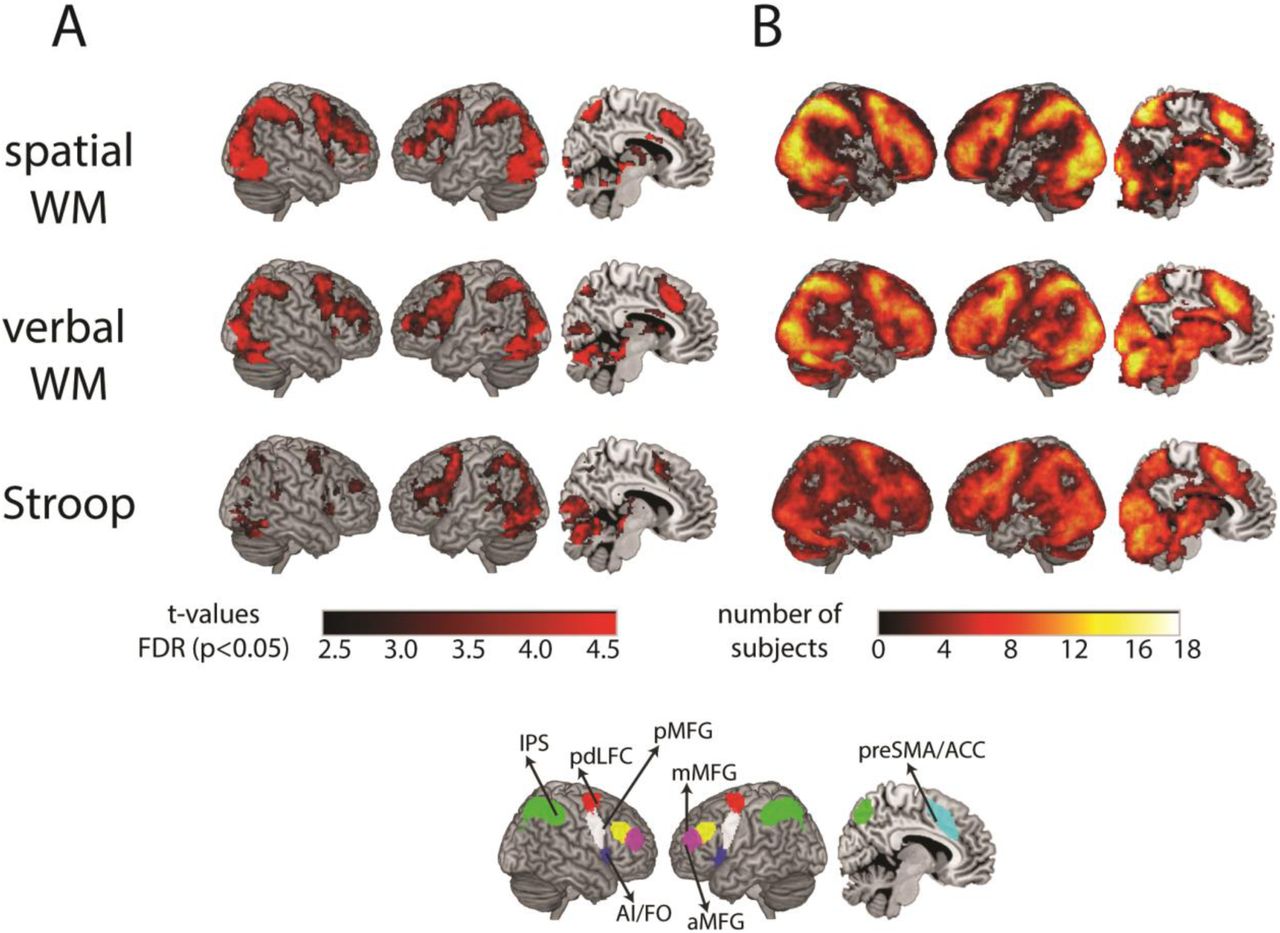
A: Whole-brain t-maps of the contrast between Hard and Easy conditions for the localizer tasks. WM = working memory. t-maps are FDR corrected, p<0.05. B: Overlap of significant activations found in single subjects demonstrates differences in activation patterns between participants. The color of each voxel shows the number of subjects that had significant activation in that voxel in the Hard versus Easy contrast, with the color bar indicating number of subjects upto to 18 (sample size), thresholded at 1 subject. Bottom panel: The MD template that was used for ROI analysis is shown for reference (adapted from Fedorenko et al. 2013).
While the average Hard versus Easy contrasts closely resembled the MD template, there was substantial variability between activation patterns of individual participants. To quantify this spread of activations across individuals, we computed a whole-brain overlay map for each localizer (Figure 2B). Each participant’s Hard versus Easy contrast was thresholded using FDR (p < 0.05). Then, for each voxel, the number of participants with significant activations was computed.
ROI analysis further confirmed the recruitment of the MD network (Figure 3). All localizers showed a significant increase in activation for the Hard compared to the Easy condition in each of the ROIs (two-tailed one-sample t-test against 0: t17 ≥ 2.57, p ≤ 0.02 for all). A three-way repeated measures ANOVA with factors task (spatial WM, verbal WM, Stroop), ROI (7) and hemisphere (left, right) revealed a main effect of task (F2, 34 = 3.96, p = 0.028). There was a significant main effect of ROIs (F6, 102 = 7.6, p <0.001) and hemisphere (F1, 17 = 15.54, p = 0.001), with larger activity on the left than the right hemisphere. There were also significant interactions between tasks and ROIs, tasks and hemispheres, ROIs and hemispheres and a three-way interaction (F > 4.1 p < 0.009). Post-hoc pairwise comparisons with Bonferroni correction (3 comparisons) across ROIs demonstrated a marginal difference in activity between the verbal WM and Stroop task (t17 = 2.64, corrected p = 0.051), but the overall activity did not differ between the spatial WM and verbal WM tasks or the spatial WM and Stroop tasks (t17 ≤ 1.25, p ≥ 0.3 for both). The tasks thus all recruited the MD network, with some differences in the activation patterns across ROIs for the different localizers. Overall, the univariate results confirmed a significant increase in activity in the MD network with increased task difficulty for all three localizers, as expected and designed.

Univariate results for the contrast between the Hard and Easy conditions for the three localizer tasks, per MD ROI and averaged across ROIs. Within each ROI and for the mean of ROIs, pairwise statistical testing between localizers were done using Bonferroni correction (3 comparisons). Significance levels above zero in each ROI and for each localizer are shown to demonstrate recruitment across the MD network. Error bars indicate SEM. spWM = spatial working memory, vWM = verbal working memory. pdLFC = posterior/dorsal lateral prefrontal cortex, IPS = intraparietal sulcus, preSMA = pre-supplementary motor area, AI = anterior insula, aMFG = anterior middle frontal gyrus, mMFG = middle frontal gyrus, pMFG = posterior middle frontal gyrus. * p < 0.05, ** p < 0.01, *** p < 0.001, + p < 0.06.
3.3 Comparisons of activity patterns between localizers
We further quantified and compared the activity patterns of the different localizers by using several distinct measures: specificity for the MD network, extent of recruitment of the network, spatial overlap across runs of individual localizers, and spatial overlap of activity between the different localizers.
3.3.1 Specificity of activity for the MD network
To test for the specificity of activity for the MD network, we computed the percentage of significant voxels lying within the MD template out of all significant voxels lying within the frontal, parietal and insular lobes (Figure 4A). The percentage of significant voxels lying within the MD template was between 33%-43% for all localizers (Mean ± SD: spatial WM: 42.9% ± 9.2; verbal WM: 42.3% ± 10.7; Stroop: 33.7% ± 11.5). A one-way repeated measures ANOVA with task as a factor revealed a significant difference between the localizers (F2, 34 = 8.82, p < 0.001). Post-hoc pairwise comparisons with Bonferroni correction (3 comparisons) showed that the Stroop task had a significantly lower percentage of significant voxels lying within the MD template than the spatial WM (t17 = 3.93, p = 0.003) and verbal WM (t17 = 3.14, p = 0.018) tasks. There was no difference between the two WM tasks (t17 = 0.29, p > 0.5). These results indicate that while all localizers yielded increased activity in the MD network, this increase was distributed and also widely observed outside the network. The expected extent of specificity of activity at the individual level, or its distribution beyond the MD network, is not known based on previous studies, as this is usually not reported. The relatively low specificity could be, at least in part, because of different patterns of activity of individual subjects when compared to a template that was generated by averaging data across many subjects. With percentages below 50%, these results could suggest that for each localizer and individual subject, activity tends to be outside the MD network more than within the MD network. This would be a misleading interpretation, as this measure does not take into account the large differences in the number of voxels in the MD network template compared to the ‘outside-MD’ and within the fronto-parietal-insular lobes areas, which is about 6.6 times fold for the latter compared to the former. The next measure that we used overcomes this bias.

A. Specificity of activation to the MD network: percentage of significantly activated voxels of each localizer lying within the MD template. B. Extent of recruitment of the MD network and the ‘outside-MD’ areas: percentage of significantly activated voxels of each localizer out of the total number of voxels in the MD network (darker bars) and similarly for the ‘outside-MD’ areas (lighter bars). C. Reliability of activation of the two runs of each localizer task, within the MD network (darker bars) and in the ‘outside-MD’ areas (lighter bars). D. Spatial overlap between the localizer tasks, within the MD network (darker bars) and in the ‘outside-MD’ areas (lighter bars). spWM = spatial working memory, vWM = verbal working memory. Error bars indicate SEM. * p < 0.05, ** p < 0.01, *** p < 0.001. Significance tests were conducted using a two-tailed paired t-test. Bonferroni correction for multiple (3) comparisons was used for differences between localizers in Figures 4A-C and pairs of localizers in Figure 4D.
3.3.2 Extent of recruitment of the MD network by individual localizers
Next, we tested for the extent of recruitment of the MD network by the localizers, as well as the recruitment levels of the ‘outside-MD’ areas (Figure 4B). For each localizer, we computed the percentage of significant voxels inside the MD network out of the total number of MD voxels. A similar measure was computed for the ‘outside-MD’ areas. The extent of recruitment within the MD network was 19.6% ± 9.4 for spatial WM, 23.5% ± 12.2 for verbal WM, and 13.4% ± 12.6 for the Stroop task (mean ± SD), while levels of recruitment outside the MD network were much lower: 4.4% ± 2.9 for spatial WM, 5.3% ± 3.1 for verbal WM, and 3.6% ± 3.8 for the Stroop task. A two-way repeated measures ANOVA with localizer (3) and the location (inside/outside MD), showed a main effect of location (F1, 17 = 99.9, p < 0.001), main effect of localizer (F2, 34 = 3.3, p = 0.048), and an interaction of the two (F2, 34 = 5.0, p = 0.012). Post-hoc tests showed greater recruitment inside vs. outside the network for all the localizers (two-tailed paired t-tests, t17 > 4.5, p < 0.001 for all). Post hoc tests with Bonferroni correction (3 comparisons) to test the main effect of localizers showed no difference between them (t17 < 2.6, p > 0.06). Post hoc tests with Bonferroni correction (6 comparisons) to investigate the interaction, comparing the localizers inside and outside MD, showed no differences between localizers inside or outside the template (t17 < 2.9, p > 0.06).
3.3.3 Reliability of activation of individual runs
In order to examine how consistently the localizer runs activated the MD network, spatial overlap between the two runs of each localizer task was computed (Figure 4C). This was an important question because highly reliable activations of one localizer task compared to another might imply a more accurate “targeting” of relevant areas/voxels by this localizer. For the spatial overlap between runs within the MD network, only significant voxels in each run within the MD template were considered. The number of voxels that were significantly activated in both runs was multiplied by two and divided by the sum of the number of voxels significantly activated during either run separately. Spatial overlap was 49.1% ± 19.3 for the spatial WM, 51% ± 22.2 for the verbal WM, and only 32.2% ± 23.6 for the Stroop task (mean ± SD). We further tested the reliability of activation between the two runs of each localizer outside the MD network by computing the same measure for voxels in the ‘outside-MD’ areas. Spatial overlap outside the MD network was 33% ± 17.2 for the spatial WM, 36.6% ± 17.9 for the verbal WM, and only 22.5% ± 17.2 for the Stroop task (mean ± SD). A two-way repeated measures ANOVA with factors localizer (3) and location (inside/outside MD) showed a main effect of localizer (F2, 34 = 3.8, p = 0.03), main effect of location (F1, 17 = 90.2, p < 0.001) with inside MD reliabilities being higher than outside MD, and no interaction of the two (F2, 34 = 2.8, p = 0.07). Post hoc tests with Bonferroni correction (3 comparisons) were done to address the main effect of the localizers averaged over both inside and outside the template. There was a marginal difference between the verbal WM and Stroop tasks (t17 = 2.6, p = 0.051) whereas other tasks did not significantly differ from each other (t17 < 2.1, corrected p > 0.1). These results demonstrate that while there is some consistent activation of the MD network by individual runs of the tested localizers, there is also substantial variability between runs. The reliability of activation was lower outside the MD network for each of the localizers (two-tailed paired t-tests with Bonferroni correction: t17 > 4.3, p < 0.001), implying that, while the localizers certainly recruit areas both within and outside the MD network, the evoked activity is more spatially focused and less variable within the network than the outside areas.
3.3.4 Spatial overlap between localizers
We further sought to assess the extent to which the different localizers activated the same voxels and computed the spatial overlap of activity between the localizer tasks (Figure 4D). Within the MD network, there was 49% ± 19.6 (mean ± SD) overlap between the spatial and verbal WM localizers. The overlap between the spatial WM and the Stroop task was 28.9% ± 18.7, and 35.5% ± 22.6 between the verbal WM and the Stroop (mean ± SD). This measure was also applied to the voxels outside the MD network to test for the spatial overlap between the localizers in the ‘outside-MD’ areas. The overlap between the two WM tasks was 31% ± 14.8, between spatial WM and Stroop was 16.8% ± 15.3 and between verbal WM and Stroop was 27.9% ± 26.8 (mean ± SD). A two-way repeated measures ANOVA with localizer pairs (3) and location (inside/outside MD) showed a main effect of localizer pairs (F2, 34 = 7.8, p < 0.001), a main effect of location with inside MD overlaps being larger than outside MD (F1, 2 = 26.6, p < 0.001), and an interaction between the two (F2, 34 = 4.3, p = 0.02). Post-hoc pairwise comparisons with Bonferroni correction (3 comparisons) indicated that the overall overlap (averaged across ‘inside MD’ and ‘outside MD’) between the spatial WM and Stroop tasks was significantly lower than the overlap between the spatial WM and verbal WM tasks and the overlap between the verbal WM and the Stroop tasks (t17 = 4.2, p = 0.002; t17 = 3.2, p = 0.016, respectively). The overlap between the spatial WM task and verbal WM task was not different from that between the verbal WM task and the Stroop task (t17 = 1.5, p = 0.48). Post hoc tests to investigate the interaction, comparing the overlap of the localizer pairs inside and outside MD, showed greater spatial overlaps between spatial WM and the verbal WM, and between spatial WM and Stroop tasks, inside the MD template than outside (two-tailed paired t-tests: t17 = 10.2, p < 0.001; t17 = 3.4, p = 0.009, respectively, Bonferroni corrected for multiple (3) comparisons), and no difference for verbal WM and Stroop (t17 = 2.0, p = 0.2). Overall, these results show that the two WM memory tasks spatially overlap at similar levels to the reliability of each individual task, while numerically the overlap of each of these with the Stroop task is smaller. The spatial overlap between localizers was lower outside the network than within it, also similar to the reliability results, providing additional evidence for the more focused activation within the MD network, despite being distributed in the areas around it as well.
3.4 Rule decoding and voxel selection using independent localizers’ data
We next used the conjunction masking approach to select voxels in the MD network for MVPA and tested its effect on decoding levels in the rule-based criterion task. Specifically, we tested whether the choice of localizer affects decoding results and whether this is different compared to results obtained when using all voxels within each ROI. We computed the decoding accuracy of all pairwise discriminations between rules. For each participant, each localizer was used to select the 200 most activated voxels within each ROI to be used in the decoding analysis. As reference, we repeated the decoding analysis when using all voxels within each ROI. Overall decoding accuracy above chance (50%) across all MD ROIs and rule-pairs were 4.3 ± 4.4, 4.4 ± 4.0, 4.1 ± 4.4 for voxel selection using the spatial WM, verbal WM and Stroop localizers, respectively (mean ± SD). These decoding levels were similar to previous studies that used a similar experimental paradigm (Crittenden et al. 2015; Smith et al. 2018). As a start, we tested whether overall decoding accuracy across all pairs of rules differed between the localizers. As reference, we also computed this split for the decoding data without voxel selection, i.e., when including all voxels from each ROI in the MVPA. A three-way repeated measures ANOVA with localizer (spatial WM, verbal WM, Stroop, all-voxels), ROI (7) and hemisphere (2) showed a main effect of localizer (F3, 51 = 2.9, p = 0.042). However, none of the post-hoc tests to compare pairs of tasks survived correction (Bonferroni correction for 6 comparisons, t17 < 2.7, p > 0.06). There was a main effect of ROIs (F6, 102 = 2.5, p = 0.025) but no interaction with localizer (F18, 306 = 0.8, p = 0.7). Overall, decoding across all pairs of conditions was similar for all localizers and when no voxel selection was done.
Our choice of criterion task has therefore enabled us to not only test for the effect of localizer type on the overall discrimination between rules, which might be too coarse to depict, but also for the relative decoding levels of the two types of discriminations, thus potentially picking up more subtle effects of the different localizers. The criterion task included discriminations between rules applied on the same category (within-category discriminations, e.g., between the gender and age rules, both applied on the faces category) and discriminations between rules applied on different categories (between-category discriminations, e.g., between the gender rule applied on the faces category and the viewpoint rule applied on the building category). Previous studies have shown that, across the frontoparietal network, discrimination of between-category rules was larger than within-category rules (Crittenden et al. 2016). Therefore, to get this more fine-grained picture of the effect of voxel selection using localizer data on rule decoding, as well as when all voxels are used for decoding, we split the decoding accuracy to within- and between-category rule discriminations (Figure 5). A four-way repeated measures ANOVA with localizer (spatial WM, verbal WM, Stroop, all-voxels), distinction type (within-category, between-category), ROI (7) and hemisphere (2) as within-subject factors was set to test for differences between localizers related to decoding of the two distinction types. There was no main effect of localizer (F3, 51 = 1.0, p = 0.4), and no interaction between distinction type and localizer (F3, 51 = 0.9, p = 0.4). A trend of main effect of distinction type (F1, 17 = 3.2, p > 0.1) was consistent with the previously reported results (Crittenden et al. 2016). There was no main effect of ROI or interaction of ROI with distinction type or localizer (F < 1.8, p = 0.09). Taken together, this indicates that decoding results for the criterion task were similar for all localizers as well as when using all voxels within each ROI, similar to the results obtained across all pairs of conditions.

Within- (lighter bars) and between- (darker bars) category rule decoding accuracy values above chance (50%) for voxel selection using the different localizer tasks and using all voxels (no localizer), per ROI and averaged across MD ROIs. Decoding accuracies were similar for all three localizers and when using all voxels, with similar differences between within- and between-category rule decoding (see Text (3.4) for statistical details). spWM = spatial working memory, vWM = verbal working memory. pdLFC = posterior/dorsal lateral prefrontal cortex, IPS = intraparietal sulcus, preSMA = pre-supplementary motor area, AI = anterior insula, aMFG = anterior middle frontal gyrus, mMFG = middle frontal gyrus, pMFG = posterior middle frontal gyrus. To demonstrate rule decoding, significant decoding accuracy above chance (50%) is shown. Error bars indicate SEM. * p < 0.05, ** p < 0.01, *** p < 0.001.
Based on these ANOVA results and to demonstrate that using localizer data for voxel selection did not change decoding levels, we conducted a Bayes factor analysis (Rouder et al. 2009), separately for each functional localizer compared to decoding with all voxels. First, the difference in classification accuracy between the between- and within-category distinctions for each functional localizer was compared to the classification accuracies with all voxels using a paired two-tailed t-test. The t-value was then entered into a one-sample Bayes factor analysis with a Cauchy scale parameter of 0.7. The Bayes factors for the spatial WM, verbal WM and Stroop localizer when compared to the decoding levels with all voxels were 0.40, 0.56 and 0.79, respectively. These results demonstrate little evidence for any difference in decoding between with and without voxel selection and suggest that using voxel selection with independent localizer data did not change decoding levels, and importantly did not come at the expense of reduced decodability.
Individual-subject localization of the MD network for voxel selection for MVPA can be done not only using one localizer task, but also using two runs of two different cognitive control-related tasks. This could be useful when, for example, a certain main task is related to more than one control aspect, and the experimenters wish to localize MD region in a way that will reflect that. To test for the effect of such an approach on decoding results, we repeated the analysis using voxel selection based on localizer data combined from two different localizers. For each pair of localizers, we used the first run of each localizer and created the Hard vs. Easy contrasts from the two runs. This yielded three combination contrasts (spatial WM + verbal WM, spatial WM + Stroop, verbal WM + Stroop), and these were used for voxel selection for the criterion task. A four-way repeated measures ANOVA with task (4: three combination contrasts and all-voxels), distinction type (within/between category), ROI (7) and hemisphere (2) as within-subject factors showed a trend of main effect of distinction type (F1, 17 = 3.3, p = 0.08). There was also a trend of main effect of task (F3, 51 = 2.5, p = 0.07), but none of the pairwise post-hoc tests survived correction for multiple comparisons (t17 < 2.3, p > 0.2), and there was no interaction of task and distinction type (F3, 51 = 1.4, p = 0.25). Overall, these results indicate that using combinations of localizer tasks for voxel selection yielded decoding results in the criterion task similar to the ones when using single localizers’ data, at least with the range of localizers that we used here.
To ensure that our decoding results are robust and not limited to the choice of classifier, we repeated the analysis using an RSA (representational similarity analysis) approach (Kriegeskorte et al. 2008; Nili et al. 2014). We used cross-validated Mahalanobis distances, namely linear discriminant contrasts (LDC). An LDC value between pair of conditions indicates the level of their discriminability, with larger values meaning better discrimination. The difference between the average LDC of all the between-category rule pairs and all the within-category rule pairs (ΔLDC) was calculated per participant and per ROI, with and without voxel selection, with ΔLDC larger than 0 as an indication for rule information. For all localizers as well as when all voxels were used, the ΔLDC was greater than zero (two tailed: t17 > 3.3, p < 0.016, with Bonferroni correction for multiple (4) comparisons), indicating that the distributed patterns of activity conveyed rule information, greater for between-category than within-category rule discriminations. This was comparable to a trend of behavioral distinctions seen in the SVM analysis. A three-way repeated measures ANOVA with ΔLDC as dependent variable and localizer (spatial WM, verbal WM, Stroop, all-voxels), ROI (7) and hemisphere (2) as within-subject factors showed no main effect of localizer (F3, 51 = 0.3, p = 0.7), indicating that discriminability was similar when using the three localizers for voxel selection and when using all voxels.
As a second control analysis, we further tested whether the decoding results using the conjunction masking approach were limited by the choice of our group template. We repeated the decoding analysis using the resting-state frontoparietal control network as the group template (Yeo et al. 2011), with voxel selection using the independent localizer data as well with all voxels. A three-way repeated measures ANOVA with localizer (4), distinction type (2) and hemispheres (2) as factors showed a main effect of distinction type (F1, 17 = 7.6, p = 0.014) as expected for the between- and within-category rules. There was no main effect of localizer (F3, 51 = 0.1, p = 0.96), or an interaction of localizer and distinction type (F3, 51 = 0.7, p = 0.6). These results confirmed the potential generalizability of the conjunction approach to the use of other group-level masks.
3.5 Effect of ROI size on decoding results
In order to examine whether decoding results depend on the number of selected voxels, as has been observed in the visual system, we performed MVPA for the decoding accuracies across all MD ROIs using different ROI sizes. ROI sizes ranged from 50 to 400, in steps of 50. A three-way repeated measures ANOVA was done with factors: localizer (spatial WM, verbal WM, Stroop), ROI size (8) and within- and between-category rule distinction (2). There was a main effect of ROI size (F7, 119 = 11.6, p < 0.001), no main effect of localizer (F2, 34 = 0.1, p = 0.9) and no interaction between ROI size and localizers (F14, 238 = 0.7, p = 0.7), with the latter indicating that the difference between ROI sizes was the same for the different localizers. We then pooled the data across the three localizers and rule distinctions in order to visualize the main effect of ROI size (Figure 6). Classification accuracies tended to be lower for the smaller ROI sizes, and particularly for 50 and 100 voxels. Overall decoding levels were stable with similar decoding accuracies for ROI size of 150 voxels and above. For all ROI sizes, classification accuracy was above chance (t > 3.4, p < 0.003).

Decoding accuracy above chance (50%) is presented for average of all the localizers, MD ROIs and category type distinctions and across all MD ROIs. The accuracy levels using all the voxels in the MD ROIs template (no voxel selection) is shown at the rightmost bar. Error bars indicate SEM. ** = p < 0.01, *** = p < 0.001.
4. Discussion
In this study we propose a conjunction masking approach in order to localize the MD network in individual subjects. We systemically compared three different functional localizers of the MD network based on their spatial spread, as well as the effect of using the localizers’ data in voxel selection for decoding using MVPA in a criterion task. A spatial WM, verbal WM and Stroop task were chosen based on previous studies that showed their consistent recruitment of the MD network (Fedorenko et al. 2013). In line with previous results, all tasks significantly recruited the MD network during Hard compared to Easy task conditions in our data, thus confirming their suitability to serve as localizer tasks. However, individual participants’ activation patterns were highly variable, demonstrating the need for an approach that takes that into account. A further assessment of the extent of the activation patterns in relation to the MD network, their specificity, and their consistency across runs showed similar results in all these measures for the three localizers. Importantly, voxel selection for MVPA using activation levels of the independent localizers’ data showed decoding results in a rule-based criterion task similar to previous studies, and these were similar for the three localizers. These preserved accuracy levels demonstrated that the increased localization at the individual subject level did not come at a cost of reduced decodability and maintained the sensitivity to detect task-related neural representations.
The primary benefit of the proposed approach is the use of both a group template that ensures spatial consistency across participants, as well as individual-subject activation patterns within the group template that provide more focused targeting of MD voxels. Using MVPA in a criterion task, we showed that the use of these subject-specific focused activation patterns maintained similar classification accuracy as observed when using all voxels for classification. The use of individual-subject localized MD regions also numerically maintained more subtle differences in decoding in the criterion task, where differences in rule decoding between between- and within-category remained the same when using localizer data and when using all voxels. Nevertheless, this individual localization did not lead to an increase in decoding levels that one might expect given the more focused MD targeting. One possible explanation for that could be a ceiling effect, with decoding accuracies around 56% when all voxels were used being relatively high to what is usually observed in the frontoparietal cortex (Bhandari et al. 2018). Alternatively, it could be that the voxelwise distributed pattern across the entire MD template captured well the information related to rule decoding in the criterion task that we used, with no need for further refinement of the voxels selected for this decoding. Either way, potentially using individual localizer data could influence decodability across the MD network in other tasks when such spatial refinement is required.
Although the second-level group maps of the three localizer tasks captured well the MD network template, the spread of activity evoked by the localizer tasks was wide and variable across participants as demonstrated in multiple measures, highlighting how coarse the group level mask is. While voxels that had significant activation in many subjects mostly matched an MD-like pattern, large areas around the network were significantly activated as well, though for a smaller number of subjects (Figure 2B). At the individual subject level, voxels with significant activity in a localizer task captured only about a fifth of the entire MD network template. Nevertheless, this spread was specific to the MD network system, with localizer activity capturing only 5% of the areas outside the MD network and within the frontoparietal-insular lobes (Figure 3B). In addition to inter-subject variability, we also observed within-subject variability between the two runs of each localizer task (Figure 3C), though this activity was specific to the MD network. Many factors could contribute to this variability, including noise in the scanner, practice effects and overall alertness in a repetitive task. Since time in the scanner is limited, localizer tasks need to be as short as possible. However, the high variability between runs imply that two runs may be required for each localizer. While the primary aim of using these measures was to characterise the activity associated with the different localizers, they clearly demonstrate that, in studies where localization is important, using independent dataset at the individual level may be necessary.
We chose the localizers for this study based on the extent and consistency of their recruitment of the MD network (Fedorenko et al. 2013). Therefore, we aimed to use tasks that will capture a core cognitive aspect associated with the MD network and will have the potential to be used as general functional localizers, rather than using tasks that will tap on different and specific cognitive domains of this network. As expected, all three localizers showed increased activity in the MD network, with similar levels of recruitment. Despite the similar results obtained for the localizers in terms of their spatial spread and decoding results, the Stroop task evoked weaker, more scattered and less MD-focused pattern of activity, similarly to a previous report (Fedorenko et al. 2013). These differences compared to the other two localizers were small and in some cases only marginally significant, but may imply that this task captured the MD network less well. This could be related to the two other tasks being working memory tasks, therefore reflecting a more similar cognitive construct to one another compared to the Stroop task that involves conflict monitoring and inhibition. Another possible explanation could be related to the difficulty manipulation in the task. While increase in difficulty level in the working memory tasks was simply controlled by increasing the number of highlighted cells in the grid or numbers, this manipulation in the Stroop task was operationally less well defined.
To ensure the generalizability of the conjunction masking approach and the proposed localizer tasks, we conducted two complementary analyses. First, we used linear discrinant analysis (LDA) in addition to SVM to measure discriminability and particularly differences between within- and between-category rule discriminations. A wide range of classification and discrimination approaches are used in the field for MVPA of fMRI data (Kriegeskorte et al. 2006, 2008; Ahlheim and Love 2018). Here, we showed that the discrimination levels in the criterion task folllowing voxel selection were similar for all localizers independent of the choice of the MVPA method. Second, to further test the efficacy of the conjunction masking approach, we used the frontoparietal network template from an fMRI resting-state parcellation as the group template (Yeo et al. 2011) in addition to the one derived from task-based data (Fedorenko et al. 2013). The classificaiton levels with voxel selection were similar for all three localizers when the resting-state group template was used, similarly to the results when the task-based template was used, thus confirming that our results do not depend on the choice of group mask. Altogether, these suggest that the three tested localizers are good candidates for localizing the frontoparietal control network in individual subjects.
Previous studies that tested for decoding across the frontoparietal control network used a variety of ways to define regions of interest. These include, among others, using all voxels within MD ROIs (Woolgar et al. 2011; Muhle-Karbe et al. 2017), defining areas of interest based on univariate or multivariate effects of part of the data of the main task and testing on another (Ester et al. 2015; Etzel et al. 2016), centering spheres on peak activation loci (Fox, Snyder, Barch, et al. 2005), using resting-state networks (Cole et al. 2013), searchlight algorithm (Cole et al. 2016), and anotomical landmarks in conjunction with group-level univariate contrast (Curtis et al. 2005). In contrast to these, the conjunction masking approach that we propose here offers a balance between the need of a consistent definition of regions across participants, and perhaps studies, and the localization at the individual participant level. Different variations of this approach can be designed for future studies depending on the research question, to be used with both univariate and multivariate analyses while avoiding double-dipping. For example, data from two localizer tasks can be combined, as we demonstrated here. The spatial overlap between runs of two different localizers was only partial, possibly reflecting differential functional preferences for cognitive demands and constructs across MD regions demands (Dosenbach et al. 2007; Nomura et al. 2010; Crittenden et al. 2016; Assem et al. 2019; Shashidhara et al., Submitted). Combining data across localizers could lead to capturing core parts of the MD system, reflecting the multiple-demand nature of the selected voxels (Duncan 2010, 2013; Fedorenko et al. 2013; Assem et al. 2019). Other variations of the our proposed approach can include the use of more than two localizers, or a localizer that consists of multiple tasks with a similar manipulation of difficulty level. On the other end of this scale, a localizer task can be designed to target a specific cognitive aspect of interst, and the use of the counjunction masking approach will ensure that the areas of interest are within the boundaries of the MD control network, thus can be related and compared to other studies.
In the proposed approach, the number of voxels that are selected to be used in MVPA can be controlled for. It has been previously shown that increased ROI size leads to increased classification levels in the visual system, highlighing the need to control for ROI size when comparing results across ROIs (Eger et al. 2008; Walther et al. 2009; Said et al. 2010). It was not clear whether this is the case for MD regions, which are different from visual regions at multiple levels, and whether more generally the choice of this parameter affects decoding levels. In our data, we observed slightly lower levels of classification for the smaller ROI sizes (50 and 100 voxels), but these stabilized for ROI sizes larger than 100 voxels, in line with previous reports (Erez and Duncan 2015; Shashidhara and Erez 2019). This does not necessarily mean that such high dimensionality is required to reach maximal decodability without over-fitting, an issue that other studies have looked into more formally and directly (Ahlheim and Love 2018). Importantly, controlling for ROI size may be essential when comparing MD regions to other brain systems, such as visual areas, further emphasising the importance of using a method that enables such control.
In summary, we propose a conjunction masking approach to localizing MD control regions, combining both a group-level mask and localizer data of individual subjects. We showed that individual patterns of recruitment of MD regions are highly variable across participants, and that the proposed approach allows for a refined, targeted localization in each participant without compromising the ability to capture task-related representations as measured with MVPA in a rule-based criterion task. This approach provides a useful way to maintain sensitivity of the broad group templates with an added specificity of activations at the individual subject level and serves as another step towards standardization and increased comparability across studies in the field.
Acknowledgements
This work was funded by a Royal Society Dorothy Hodgkin Research Fellowship (UK) to Yaara Erez (DH130100). Sneha Shashidhara was supported by a scholarship from the Gates Cambridge Trust, Cambridge, UK. Floortje Spronkers was supported by an Erasmus+ Traineeship grant and a Stichting A.S.C. Academy grant. We thank John Duncan and Daniel Mitchell for fruitful discussions and advice throughout the study.
The authors declare no competing financial interests.
Footnotes
↵* Equal contribution


