

Abstract
Confidence intervals (CIs) depict the statistical uncertainty surrounding evolutionary divergence time estimates. They capture variance contributed by the finite number of sequences and sites used in the alignment, deviations of evolutionary rates from a strict molecular clock in a phylogeny, and uncertainty associated with clock calibrations. Reliable tests of biological hypotheses demand reliable CIs. However, current non-Bayesian methods may produce unreliable CIs, because they do not incorporate rate variation among lineages and interactions among clock calibrations. Here, we present a new analytical method to calculate CIs of divergence times estimated using the RelTime method, along with an approach to utilize multiple calibration uncertainty densities in these analyses. Through empirical data analysis, we show that the new methods produce CIs that overlap with Bayesian highest posterior density (HPD) intervals. These developments will encourage broader use of computationally efficient, non-Bayesian relaxed clock approaches in molecular dating analyses and biological hypothesis testing.
Introduction
Reliable inference of the confidence intervals around the estimates of divergence times is essential for testing biological hypotheses (Burbrink and Pyron 2008; Kumar and Hedges 2016). Multiple sources contribute to the uncertainty of molecular divergence time estimates (Rannala and Yang 2007; Zhu et al. 2015; Kumar and Hedges 2016). One of them is the error associated with branch length estimation in a phylogeny due to the limited number of sites and substitutions in the sequence alignment (Kumar and Hedges 2016; Warnock et al. 2017). The stochastic nature of the substitution process (e.g., Poisson process) and the uncertainty involved in accounting for the unobserved substitutions (multiple-hit correction) result in errors in branch length estimates, which lead to imprecise time estimates (Kumar and Hedges 2016). However, this error decreases with an increase in the number of sampled sites (Rannala and Yang 2007; dos Reis and Yang 2013; Zhu et al. 2015) and becomes negligible for large phylogenomic datasets. A second source of error is the variation of evolutionary rates among branches and lineages (Zhu et al. 2015; Kumar and Hedges 2016). Because rates and times are confounded, the variation of rates will naturally result in uncertainty of time estimates (Ho 2014; Zhu et al. 2015). This confounding effect cannot be eliminated by sampling more sites or genes in a dataset (Zhu et al. 2015; Kumar and Hedges 2016), so it contributes more uncertainty to time estimates than errors in branch length estimation for a large dataset. The uncertainty associated with clock calibrations due to the equivocal nature of fossil record presents a third source of error in divergence time estimation (Zhu et al. 2015; dos Reis et al. 2016; Warnock et al. 2017). The exact placement of fossil record in a phylogeny and the correct assignment of calibration constraints, especially the maximum constraint, are often difficult to justify, resulting in great uncertainty in estimation of divergence time (Bromham et al. 2018).
In Bayesian analyses, the highest posterior density (HPD) intervals usually represent the uncertainty of inferred divergence times (Drummond et al. 2006). Bayesian methods compute HPD intervals directly from the density distribution of posterior times estimated using priors for rate heterogeneity, substitution process and fossil calibrations (dos Reis et al. 2016; Bromham et al. 2018), so sources contributing to the uncertainties of time estimates are automatically incorporated in the HPD intervals. Currently, Bayesian HPDs are considered reliable estimates of uncertainties surrounding divergence time estimates. However, the large computation burden imposed by Bayesian approaches has hindered their applications to analyze many phylogenomic datasets (Pyron 2014; Mello et al. 2017; Li et al. 2019).
In contrast, non-Bayesian methods can analyze large-scale datasets quickly and generate accurate time estimates (Smith and O’Meara 2012; Tamura et al. 2012; Tamura et al. 2018). Unfortunately, the broad utility of these methods is still reduced by lack of reliable calculation of the uncertainty surrounding divergence times, which are represented by confidence intervals (CIs). Non-Bayesian approaches require the use of analytical formulations or bootstrap approaches to estimate CIs (Sanderson 2003; Xia and Yang 2011; Tamura et al. 2013). However, site-resampling bootstrap approaches do not capture the error caused by rate heterogeneity, leading to false precisions of time estimates. Recognizing the need for incorporating lineage rate variation into CIs, Tamura et al. (2013) formulated analytical equations for the RelTime method, a non-Bayesian approach that relaxes the molecular clock. However, this approach may overestimate the amount of variance and produce overly wide confidence intervals (see below), resulting in low power for statistical testing (Kumar and Hedges 2016).
Bayesian and non-Bayesian methods also use different strategies to account for the uncertainty of fossil record. Non-Bayesian methods are limited to the use of minimum boundaries only, maximum boundaries only, or minimum and maximum boundary pairs as calibration constraints (Sanderson 2003; Tamura et al. 2013), while Bayesian methods allow the usage of informative probability densities as calibrations and automatically accommodate interactions among them (Inoue et al. 2010; Ho and Duchêne 2014). Mello et al. (2017) presented a simple procedure to derive minimum and maximum boundaries from the density distributions, but this strategy does not consider interactions among calibrations and may lead to overestimates of the variance of divergence times (see below).
Here, we present an analytical approach to estimate CIs for divergence times estimated with RelTime, accounting for variance associated with the branch lengths estimation and variance due to rate heterogeneity. We also present a simple approach to derive minimum and maximum boundaries from multiple calibration densities and accommodate calibration interactions. Both methods have been implemented in MEGA X for use in graphical and command line interfaces (Kumar et al. 2012; Kumar et al. 2018). The 95% CIs produced by RelTime in empirical analyses are compared with the 95% HPD intervals produced by Bayesian methods to examine the performance of the new approaches. The approach presented here may be used to improve variance calculation of time estimates for other non-Bayesian methods, e.g., penalized likelihood methods (Sanderson 2003; Smith and O’Meara 2012).
New Methods
An analytical method to estimate confidence intervals
Considering a tree with three ingroup sequences (Fig. 1), relative time (t) for each node and relative rate (r) for each lineage are functions of branch lengths (b) in RelTime, e.g., r1, r2, r3, r4, t4, and t5 are given by the following equations when the geometric means are used (similar equations can be derived when the arithmetic mean is used) (Tamura et al. 2018):


An evolutionary tree of three tips showing node times (ti’s), branch lengths (bj’s), and branch rates (rj’s).
The variance of the estimated time (ti) for node i, denoted by ν(ti), can be estimated by the delta method, assuming that there is no covariance among branch lengths (bj’s):
 where
where  stands for the analytical function of bj’s to compute ti (e.g., eq. 5 and eq. 6 for t4 and t5, respectively), and ν(bj) stands for the variance of branch length for branch j. Therefore, ν(bj) is required for computing ν(ti).
As mentioned before, the uncertainty of time is related to the number of sampling sites and the degree of rate heterogeneity. We consider the total variance of branch lengths, ν(bj), which is required to compute ν(ti), as a summation of the variance due to site sampling, νs(bj), and the variance due to rate heterogeneity, νR(bj):

The value of νs(bj) can be estimated by using analytical formulations or a site-resampling approach. For example, an approximate estimate of this variance can be obtained by the curvature method when the maximum likelihood method is used (Edwards 1992; Tamura et al. 2013).
However, it is more complex to estimate νR(bj), so we do it indirectly. We first compute the variance of observed evolutionary rates for all the lineages, Vobs(R):
 where R is a random variable representing all relative rates, rj is the relative rate for each branch j, and
  is the average of rj’s. It is important to note that the relative rate for branch j is estimated as the relative rate for lineage j (Tamura et al. 2018). For example, RelTime computes the relative rate for b4 as the geometric mean of r1 and r2, which is assigned to be the rate for lineage l4 in Figure 1.
The variance of observed rates includes not only the variance introduced by rate heterogeneity, RV(R), but also the sampling variance associated with the branch length estimation, sV(R), because the observed relative rate rj is calculated from branch lengths (bj’s) (e.g., equations 1 - 4). So,

The value of sV(R) is obtained by summing the sampling variance of relative rate rj for each branch j, denoted by sν(rj):
 sν(rj) can be estimated by the delta method, assuming that there is no covariance among bj’s:
 where
where  stands for the analytical function of bj’s to compute rj (e.g., equation 1, 2, 3 and 4 for r1, r2, r3, and r4, respectively).
Using equations 9 – 12, we compute the variance introduced by rate heterogeneity: 6

Then, we can compute the rate heterogeneity variance for each branch j as being proportional to its branch length:

Using equations 8, 13 and 14, we can compute the total variance of branch length for branch j, denoted by ν(bj). Then ν(bj) can be used to compute the variance of time, ν(ti), using equation 7. For example, the variance of t4 and t5 are given by the following equations:


For larger numbers of taxa, such analytical formulations become complicated to derive, especially for deeper nodes. Thus, we compute the variance of divergence times for deeper nodes from tips to the root recursively. For example, using equations 15 and 16, we can derive

Therefore, the calculation of ν(t5) requires only ν(t4), ν(b3) and ν(b4), which are the variance for node t4 and branches b3 and b4, respectively. Variance of branches that do not directly connect to node 5, i.e., ν(b1) and ν(b2) in this case (Fig. 1) is not needed, if the value of ν(t4) is computed beforehand. Thus, for any node in a phylogeny, we can compute the variance of divergence time recursively from tips to the root by using the variance of times for direct descent and ancestral nodes and the variance of direct connected branches. This procedure extraordinarily simplifies the computation of the variance of inferred time for each internal node in a tree with a large number of taxa.
It is important to note that times in the equations listed above are relative times, not absolute times because no calibrations are involved in the above equations. When one or multiple calibrations (minimum boundaries only, maximum boundaries only, or minimum and maximum boundary pairs) are given, RelTime will compute a global time factor (f) by altering relative times such that all calibration constraints are satisfied. When a range of f values can satisfy all calibration constraints, RelTime selects the midpoint of the range to be the best estimate of f. When one or more of the absolute times computed using the f value falls outside the calibration constraints, then RelTime adjusts relative times and f such that the deviations of absolute times from the calibration constraints are minimized. This process requires local alteration of relative rates and re-optimization of all other node times in the tree recursively (Tamura et al. 2013). For example, if the minimum age constraint of a node is violated, i.e., the age estimated using f is younger than the minimum constraint, RelTime decrease its estimate of the evolutionary rate proportionally in that lineage to adjust the age of this node to be higher, such that the divergence time becomes the same as the minimum age constraint. The resulting slowdown is transmitted to all the descendant nodes, and it affects the ancestral rates as well.
Similarly, if the maximum age constraint of a node is violated, i.e., the age estimated using f is older than the maximum constraint, RelTime increases the estimated evolutionary rate proportionally in that lineage such that the divergence time matches the maximum age constraint. Effects of this rate change will be transmitted to the descendant and ancestral nodes automatically. Consequently, RelTime will ensure that the absolute times for calibrated nodes are consistent with the user-desired calibration constraints. In the final step, CIs are computed analytically using the final set of relative rates and the equations given above (e.g., equations 13–17), such that the uncertainty associated with clock calibrations can be incorporated into the CI calculation in RelTime. If the lower or upper bounds of CIs fall outside the user-specified calibration constraints, then CIs are truncated based on the imposed calibration constraints. Therefore, RelTime uses “hard” minimum and maximum bounds, as in BEAST (Bouckaert et al. 2014; Barba-Montoya et al. 2017).
A method to derive effective calibration boundaries from calibration densities
As stated above, calibration uncertainty is another critical source of uncertainties in divergence time estimates. Bayesian methods use various probability densities to accommodate the calibration uncertainty. However, the current non-Bayesian methods do not allow direct usage of probability densities and do not incorporate interactions among calibration constraints. Therefore, we developed a new procedure for use in the RelTime method to derive calibration boundaries from probability densities and account for calibration interactions.
For each calibrated node with an associated probability density, we randomly sample two dates from the given probability density. We use these two sampled dates as the minimum and maximum (min-max) constraints for that node and derive such a min-max constraint for every node for which a probability density is specified. Then, we use all of these min-max boundaries in the RelTime analysis. We save the RelTime time estimates only for the calibrated nodes. This random sampling and dating process is repeated 10,000 times. Therefore, we will have generated a distribution of 10,000 inferred dates for each calibrated node. In the final step, we derive the minimum bound at 2.5% and the maximum bound at 97.5% of the distribution of inferred dates for each calibrated node. We refer to these derived bounds as “effective bounds.” These effective bounds can be used together with the analytical approach described above to infer the divergence times and CIs in RelTime. It is important to note that effective bounds are used as calibration constraints, not densities. The actual distribution of 10,000 inferred dates does not impact the value of effective bounds and therefore, the final RelTime estimates of divergence times and CIs.
Our procedure is analogous to how Bayesian methods utilize calibrations, as both types of methods require resampling different sets of calibration constraints from user-specified densities, inference of divergence times using each set of sampled calibrations, and summarization of distributions of time estimates obtained from all sets of sampled calibrations. Therefore, the use of effective bounds allows RelTime to accommodate the interactions among calibration densities. However, it does not mean that RelTime and Bayesian methods are the same. Bayesian methods conduct calibration resampling and time inference steps simultaneously during the MCMC integration, whereas these steps are implemented sequentially in the RelTime method.
We compare the effective bounds to calibration bounds derived using Melloetal.(2017)’s procedure(referenced as”Mellobounds”in thefollowing)(Fig. 2),in which the minimum bound was placed at 2.5% of the density age, and the maximum bound was placed at 97.5% of the density age. Effective bounds are similar to the Mello bounds when the user-specified calibration density is reliable and informative(Fig. 2b, see Materials and Methods).When the user-specified density is uninformative, e.g.,a diffused uniform distribution,Mello bounds are often diffused and match the original density(Fig. 2c).However,our procedure generate snarrower bounds due to the accommodation of the interactions among different calibration densities and constraints. These interactions reshape the original, wider distribution to be tighter (Fig. 2c). Consequently, the use of effective bounds is likely to produce more precise time estimates (narrower CIs). When the user-specified calibration is unreliable, our effective bounds turn out to be better than Mello bounds. For example, if the true time is located in the user-specified density with a low probability (< 2.5%), Mello bounds may not include the true time (Fig. 2d), resulting in incorrect time estimates. In contrast, our method does not ignore the low probability regions since it samples 10,000 times from the user-specified density to ensure that dates with very low probabilities may be sampled. Thus, effective bounds should contain the true time (Fig. 2d), and the use of effective bounds in RelTime should improve the accuracy and precision of time estimates.

(a) A primate phylogeny with a user-specified uniform calibration density (gray shade) and an exponential calibration density (green shade). Red dots are the nodes shown in panels b-d. Effective bounds derived using our method (solid blue line) and bounds derived using Mello et al. (2017) procedure (solid orange line) are compared (b and c) when user-specified calibrations are reliable and (d and e) when user-specified calibration of Homo-Callithrix split is unreliable. The dashed red line represents the “true simulated age.”
Results and Discussion
We applied our methods to three empirical datasets, including nucleotide or protein sequences from primates, spiders, and insects (Table 1). We begin with the primate dataset from Barba-Montoya et al. (2017), which contains a relatively small alignment of 9,361 base pairs from nine primate species and one outgroup (Fig. 2a). However, all internal nodes were assigned with calibration densities. Barba-Montoya et al. (2017) used two calibration strategies in MCMCTree (Yang 2007) and BEAST (Bouckaert et al. 2014) and compared the results. We examined if the RelTime method produced estimates comparable to those obtained from Bayesian methods, when all analyses employed the same alignment, phylogeny, substitution model, and calibration uncertainty densities (e.g., uniform distributions).
Empirical datasets analyzed in this article
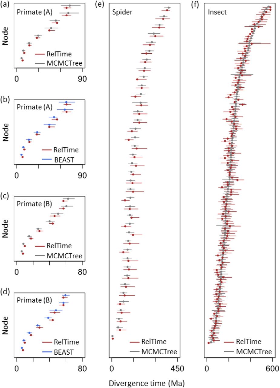
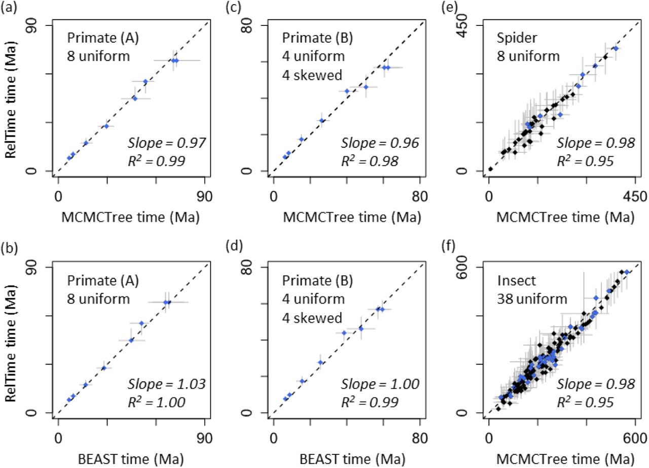
For analyses of primate datasets where uniform densities were used as calibrations, we observed a high concordance between RelTime and Bayesian time estimates. The linear regression slopes were 0.97 and 1.03 when Bayesian analyses were conducted in MCMCTree and BEAST, respectively (Fig. 3a and b). This a rather small difference. Although the width of RelTime CIs was slightly smaller than the width of Bayesian HPD intervals, RelTime CIs overlapped Bayesian HPD intervals for all the nodes (Fig. 4a and b). For primate datasets where a mixture of uniform and skewed densities were used as calibrations, RelTime estimates were again similar to Bayesian estimates, with a linear regression slope of 0.95 with MCMCTree (Fig. 3c) and 1.00 with BEAST estimates (Fig. 3d). RelTime CIs overlapped with MCMCTree and BEAST HPD intervals for all the nodes (Fig. 4c and d).

Comparisons of RelTime and Bayesian estimates of divergence times and the associated uncertainties. Gray bar represents the Bayesian 95% HPD intervals (x-axis) and RelTime 95% CIs (y-axis). Black dashed line represents 1:1 line. Each graph contains the slope and coefficient of determination (R2) values of the linear regression through the origin. Calibrated nodes are shown in blue. The dataset name inside each panel refers to table 1.
Comparisons of RelTime 95% CIs (dark red), MCMCTree 95% HPD intervals (gray) and BEAST 95% HPD intervals (blue). Dots are point estimates of divergence times. The dataset name inside each panel refers to table 1.
We then analyzed spider and insect datasets to examine the performance of our methods for larger datasets (>40 species and >50,000 sites). These datasets consisted of protein sequences; 8 nodes had clock calibrations for the spider data, while 38 nodes of the insect phylogeny were assigned calibration values. We again observed strong concordance between RelTime and Bayesian time estimates, with a linear slope of 0.98 and 0.98 for spider and insect data, respectively (Fig. 3e and f). The high similarity between RelTime and Bayesian node times remained even after we excluded nodes on which user-specified calibrations were assigned (slope = 0.97 and 0.98, respectively). CIs produced by RelTime were also comparable with HPD intervals produced by Bayesian methods, with more than 97% of the nodes in spider and insect datasets showing overlapping CIs and HPD intervals (Fig. 4e and f). When CIs and HPD intervals did not overlap, they were less than 5 million years apart. Therefore, we considered that RelTime CIs were similar to Bayesian HPD intervals for all datasets.
Our new methods allow RelTime to produce point time estimates and CIs similar to those inferred by Bayesian methods across all empirical analyses because our new methods effectively improve the CI calculation. We found that, on average, our analytical approach produced CIs that were 35% - 67% narrower than those produced by Tamura et al. (2013)’s method without any calibrations. However, time estimates remain very similar between these two methods with linear slopes ranging from 1.00 to 1.02. These results show that the use of the new analytical approach solely can effectively improve the precision of time estimates in RelTime while maintaining the same accuracy.
We also compared time estimates and CIs produced by the new analytical approach with effective bounds generated by our new procedure and calibration bounds generated by Mello et al. (2017)’s procedure. This comparison would illuminate how the use of effective bounds may improve the precision of divergence time estimates. Results showed that times estimated using two sets of calibration bounds were similar (linear slopes ranging from 0.99 to 1.02). However, the CI width was reduced by 7-29% when effective bounds were used. The decrease of CI widths occurred for both calibrated and uncalibrated nodes. It is because effective bounds reflect calibration interactions and reshape the original diffused calibration densities to generate narrower CIs, as discussed above. Therefore, both of our methods improve the precision of divergence time estimates produced by RelTime without sacrificing their accuracy.
It remains important to note that reliable time estimates and CIs rely strongly on the assumption that calibrations and their densities are correct. The incorrect specification of calibration constraints or densities can greatly impact the accuracy and precision of time estimates (Warnock et al. 2017). Our empirical analyses showed that RelTime and Bayesian methods generated similar estimates of divergence times and their surrounding uncertainties when the same alignment, phylogeny, and calibration densities were used. These patterns indicate that RelTime can serve as a reliable alternative to Bayesian approaches for dating the tree of life and conducting biological hypothesis testing, especially for large-scale molecular data, because RelTime is computationally efficient, requiring only a fraction of the time and resources demanded by Bayesian approaches (Tamura et al. 2012; Tamura et al. 2018). We also anticipate that our method of deriving effective bounds from calibration densities can be applied to other non-Bayesian dating methods, e.g., penalized likelihood methods (Sanderson 2003; Smith and O’Meara 2012).
Materials and Methods
Comparisons of user-specified calibration density, Mello bounds, and effective bounds
We used the BEAST-generated primate timetree published in Barba-Montoya et al. (2017) as the true tree (Fig. 2a) and simulated an alignment of 9361 sites under HKY+G (Hasegawa et al. 1985) model in SeqGen with parameters derived from the empirical molecular data. Branch-specific rates were sampled from an uncorrelated lognormal distribution with a mean rate of 0.0069 substitutions per site per Ma and a standard deviation of 0.4 (log-scale). The simulated alignment was used to derive effective bounds.
We tested the performance of using effective bounds and Mello bounds under two calibration scenarios: reliable and unreliable scenarios. An informative exponential density was used at homo sapiens – Callithrix jacchus split (true age = 44.8Ma) and an uninformative uniform density were used at homo sapiens – Otolemur gamettii split (true age = 68Ma) under both scenarios. In the reliable calibration scenario, we assumed that a minimum age of 40Ma at homo sapiens – Callithrix jacchus split and maximum age of 130Ma at homo sapiens – Otolemur gamettii split are known. Therefore, we used an exponential density (mean = 4Ma and offset = 40Ma) and a uniform density (min = 40Ma, max = 130Ma) at homo sapiens – Callithrix jacchus split and at homo sapiens – Otolemur gamettii split, respectively. The true ages of both nodes located in their densities with high probabilities. Under the unreliable calibration scenario, we assumed that a minimum age of 30Ma at homo sapiens – Callithrix jacchus split and maximum age of 130Ma at homo sapiens – Otolemur gamettii split are known. Therefore, we used an exponential density (mean = 3Ma and offset = 30Ma) and a uniform density (min = 40Ma, max = 130Ma) at homo sapiens – Callithrix jacchus split and at homo sapiens – Otolemur gamettii split, respectively. This results in the true age of homo sapiens – Callithrix jacchus split located in its density with a low probability (< 2.5%), while the true age of homo sapiens – Otolemur gamettii split located in its density with a high probability.
Empirical analysis
We obtained four empirical datasets that employed different calibration strategies from three published studies (Table 1) (Bond et al. 2014; Tong et al. 2015; Barba-Montoya et al. 2017). Molecular data were obtained from supplementary files of original studies. Calibration densities and Bayesian timetrees (including credibility intervals) of Barba-Montoya et al. (2017) and Tong et al. (2015) were provided by authors. For Bond et al. (2014)’s data, we obtained the Bayesian timetree (including HPD intervals) from Mello et al. (2017). In RelTime analyses, we used the same alignments, substitution models, tree topologies, and calibration densities as the original studies to ensure comparability with Bayesian results. RelTime analyses were conducted in MEGA X (Kumar et al. 2018). We compared RelTime time estimates and CIs with Bayesian time estimates and HPD intervals. We did not test whether the slope between RelTime and Bayesian time estimates was one because of two reasons. First, p-value will always reject the hypothesis of slope of one when the data sample size is large. Second, the uncertainty surrounding time estimates prevents time estimates from two types of methods to be identical. We also compared the performance of our methods and the previous CI calculation method for RelTime. We first reanalyzed all empirical datasets using Tamura et al. (2013)’s method in MEGA 7 (Kumar et al. 2012; Kumar et al. 2016) and using our analytical method in MEGA X without calibrations. We then re-analyzed all empirical datasets in MEGA X using the effective calibration bounds generated by our new method and by Mello et al. (2017)’s procedure.
Acknowledgments
We thank Drs. Jose Barba-Montoya and Simon Ho for sharing Bayesian results. We thank Drs. Sayaka Miura and Jose Barba-Montoya for critical comments. This research was supported by grants from the National Institutes of Health (NIH GM0126567-02), National Science Foundation (NSF 1661218), and National Aeronautics and Space Administration (NASA NNX16AJ30G) to SK, Brazilian Research Council (CNPq 233920/2014-5 and 409152/2018-8) to BM, and Tokyo Metropolitan University (DB105) to KT.
References


