

Abstract
Modelling genetic diversity needs an underlying genealogy model. To choose a fitting model based on genetic data, one can perform model selection between classes of genealogical trees, e.g. Kingman’s co-alescent with exponential growth or multiple merger coalescents. Such selection can be based on many different statistics measuring genetic diversity. We use a random forest based Approximate Bayesian Computation to disentangle the effects of different statistics on distinguishing between various classes of genealogy models. For the specific question of inferring whether genealogies feature multiple mergers, we introduce a new statistic, the observable minimal clade size, which corresponds to the minimal allele count of non-private mutations in an individual.
1. Introduction
Modelling genetic diversity of a sample of present-day individuals is a key tool when reconstructing the evolutionary history of populations or scanning the genome for regions under selection, see e.g. [CB17, Section “Nonequilibrium theory”, p. 1026]. For a genetic region without recombination, a standard approach is to model the genealogical tree and the mutations along its branches as random processes. The genealogy thus is given by a n-coalescent, a random tree with n leaves. On this, mutations are modelled as an independent Poisson process along the edges of the coalescent tree. Several genealogical models have been proposed. The most widely used model, Kingman’s n-coalescent, approximately describes the genealogy of a fixed-size population under neutral evolution if offspring numbers per parent are not too variable, e.g. if the population is described by a (haploid or diploid) Wright-Fisher model or a Moran model with fixed size N. More precisely, the n-coalescent is the limit (in distribution) of the genealogies in the discrete populations as N → ∞, if one treats  generations as one unit of time in the coalescent tree (which has a continuous time scale). Here, cN is the coalescence probability, i.e. the probability that two individuals, picked in any generation, have a common parent. Variants of Kingman’s n-coalescent as limits of genealogies from Wright-Fisher models with varying population size and/or population structure are available, see e.g. [GT94], [WH98]. These variants still are strictly bifurcating trees. Barring recombination, both haploid and diploid populations are well-captured by Kingman’s n-coalescent and its variants.
However, some populations will feature genealogies not well approximated by Kingman’s n-coalescent and its bifucating variants. Certain modes of rapid selection, affecting the whole genome should lead to the Bolthausen-Sznitman n-coalescent, e.g. see [NH13], [DWF13], [Sch17]. This genealogy model likely produces multifurcating genealogical trees. Even a succession of hard selective sweeps may cause a multifurcating genealogy (though not the same model), see [DS05].
Generally, if one considers the genealogy in an arbitrary Cannings model, a fixed-size discrete-time population model where offspring sizes are exchangeable among parents, a whole class of multifurcating trees, the Λ- or Ξ-n-coalescents, emerges as possible weak limits of the genealogies for N → ∞, again with the analogous rescaling as for Kingman’s n-coalescent, see [MS01]. Non-Kingman n-coalescents arise if the distribution of offspring size per parent is variable enough, see [Möh98]. They have been shown to explain the genetic diversity of several maritime species better than Kingman’s n-coalescent and its variants, see e.g. [EW06], [NNY16] or [HSJB19]. They seem to capture well the concept of sweepstake reproduction, where one individual may produce a considerable part of the population by chance. Two specific haploid models proposed for this are leading to the Eldon-Wakeley n-coalescents, see [EW06], and to the Beta-n-coalescents, see [Sch03]. However, for multiple merger coalescents diploid population should be modelled by variants of the haploid n-coalescents, see [BLS18]. Again, variants for changing population sizes in the pre-limit models are available, see [MHAJ18], [Fre19], [KWB19], [GCMPSJ19]. For further discussion where multiple merger genealogies may arise, see the reviews [TL14] and [ILM+16]. How can one distinguish these genealogical models based on a sample of n genomic sequences? Available methods using the full sequence information do not scale well with data sets with many individuals and/or regions with many mutations [SBB13], [Ste09], [Kos18]. Thus, less costly methods based on a summary statistic of the genomic information, the site-frequency spectrum (SFS), have been proposed, see e.g. [EBBF15], [Kos18]. These methods are noisy for one or few regions, but have fairly low error rates for data taken across the genome for many unlinked loci, see [Kos18]. However, even whole genomes may not contain many unlinked loci. For instance, many bacterial genomes consist of a single chromosome with neglectable recombination, e.g. in Mycobacterium tuberculosis, also several fungi have comparably small genomes with large linkage blocks.
For cancer cells, (one-locus) Beta-n-coalescents with exponential growth have been proposed as a genealogy model for copy numbers (specific mutations) in cancer cells [KVS+17] within multiple regions. In this study, quantiles of the SFS and several additional statistics were used as summary statistics for inference based on Approximate Bayesian Computation (ABC). Low misclassification errors (≤ 2%) were reported, which were much lower than the SFS-based misclassification errors from [EBBF15]. The discrepance of error rates may come from slightly different hypotheses, a different approach to mutation rates, a different ABC approach and/or the use of additional summary statistics.
Motivated by this drop in error rates, our goal is to investigate which statistics are best suited to distinguish different classes of n-coalescents. Additionally to the statistics from [KVS+17], we consider some further common statistics as well as a new statistic, the smallest allele frequency among nonprivate mutations observed in one individual.
These statistics are used in an ABC framework. We use a slight modification of the ABC approach based on random forests from [PME+15] that performs well with many, potentially uninformative statistics and that measures the importance of each statistic to distinguish between the hypotheses.
1.1 Methods
The genealogical trees are all given by Λ- or Ξ-n-coalescents, which are random trees with a Markovian structure. We start with n leaves at time 0 and build the tree until its root is reached. If b branches are present at a time t, k of these, chosen at random, will be merged with rate λb,k. In the case of Λ-n-coalescents, k lines are merged into one new line, in other words they are joined in a node of the tree and a new branch towards the root is started. These rates are characterized by
 with a finite measure Λ on [0, 1], see [Pit99]. For Ξ-n-coalescents, k = (k1, …, km) sets of lineages are each merged into one new line, so m new nodes are added from which m new branches extend (the new node i has thus in-degree 1 and outdegree ki). The rate
  of such a merger can be expressed in terms of a finite measure Ξ on the simplex, as introduced in [Sch00].
As introduced above, all n-coalescents can be seen as limit trees of genealogies of a sample size n in discrete populations of fixed size N → ∞ across all generations. If population size may change, but stays of order N across generations, the genealogy tree is then given by a n-coalescent characterized by the same measure as in the fixed size case, but with time changed by a deterministic function, see [GT94], [MHAJ18],[Fre19],[KWB19]. As Λ-coalescent model classes, we consider Kingman’s n-coalescent, Dirac n-coalescents with Λ = δp for p ∈ (0, 1], which are a subclass of Eldon-Wakeley n-coalescents, and Beta-n-coalescents with Λ = Beta(2 −α, α) for 1 ≤ α ≤ 2. For the first two classes, we also consider exponential growth with rate ρ, which results in time change t ↦ (γρ)−1 (eγρt − 1). The parameter γ = 1 is used for Kingman’s n-coalescent [GT94], whereas we choose γ = 1.5 for the Dirac n-coalescent [MHAJ18]. We also consider one class of Ξ-n-coalescents, the Beta-Ξ-coalescents from [BCEH16] and [BLS18]. To assess population structure as a confounding factor, we also consider the structured (Kingman’s) n-coalescent with exponential growth. We assume 2 subpopulations with equal size, symmetric migration with scaled migration rate m (in units of 4N) and samples of sizes n1, n2 from each subpopulation summing up to n. See Table 1 for the short names for each coalescent model class and its (theoretical) parameter ranges.
Coalescent classes and parameters ranges
1.2 Simulation of coalescent models
We use discretized parameter ranges for simulation of each model class, see Table 2. For setting the mutation rates, we use several approaches. To be consistent with [KVS+17], for a scenario comparable to their setup we use a predefined mesh of mutation rates θ, identical for all model classes considered. However, the distribution of total length of coalescent processes differs strongly between (and within) model classes, and thus does the total number of mutations. If statistics are strongly affected by the mutation rate, this may either lead to a bad fit to the observed genetic diversity (since the parameter range used simply produces too many or too few mutations for specific models), or parameter ranges have to be very large to counteract these effects. In our case, most statistics are relatively sensitive to changes in the mutation rate. To make models comparable, we start with setting the mutation rate in each model s.t. the mean number of mutations s observed is identical. In other words, we assume, as e.g. in [EBBF15], an (integer) number s of observed mutations and set θ as the generalized Watterson estimator  , where Ln is the total branch length in the specific model we are looking at, so choosing different coalescent parameters will cause different θ values within one model class. Naturally, we do not know the true mutation rate, so we should allow some fluctuation of θ for each model. We do this either by picking the number s of observed mutations uniformly from a set of integers, or by ‘blurring’ it by drawing the mutation rate from [10−1θw(s), 10θw(s)] for one fixed value of s. We do the latter by a discrete prior symmetric on a log scale. We first draw X from a binomial distribution B(10, 0.5) and set the mutation rate to θw(s)10(X−5)/5. The specific scenarios for all three choices for mutation rates are shown in Table 3. All scenarios 1-5, consisting of specific choices of coalescent model × sample size × n mutation model are simulated twice with 175,000 times with uniform prior on the model class parameter and on either the mutation parameter θ, s or the interval of potential mutation rate choices.
Simulation settings - model classes
Simulation settings - mutation models
For simulation of 𝕂, 𝕂-exp, 2p.5-𝕂-exp and 2p.9-𝕂-exp, we perform simulations with Hudson’s ms, implemented in the R package phyclust [Che11]. 𝔻, 𝔹 and Ξ-𝔹 were simulated with R (code currently available on request, but will be put in a public repository soon). 𝔻-exp was simulated as described in [MHAJ18], using the implementation available at https://github.com/Matu2083/MultipleMergers-PopulationGrowth. Watterson’s estimator for 𝕂 is  , where s is the number of observed segregating sites. For 𝔹, 𝔻 and 𝕂-exp, we use a recursive computation approach for
  as described in [EBBF15], available from http://page.math.tu-berlin.de/~eldon/programs.html. For 𝔻-exp, we again use a recursive approach as described in [MHAJ18] (url as above). For Ξ-𝔹, we implemented the recursion from [Möh06, Eq. 2.3] in R (code currently available on request, but will be put in a public repository soon). For 2p.5-𝕂-exp and 2p.9-𝕂-exp, we approximate the expected length by averaging the total length of 10,000 simulated n-coalescents for each parameter set (again via ms).
1.3 Summary statistics
Each simulation produces a matrix with elements in {0, 1} with n rows and a variable number s of columns. The rows and columns correspond to the number of simulated sequences and to the number of mutations therein. We thus call it a (simulated) SNP matrix. We use a variety of standard summary statistics from population genetics, mostly as in [KVS+17], but also introduce a new statistic. All statistics depend on the coalescent model, θ and n. For sake of readability, we omit this dependence in the notations.
The standard statistics are all based on the following four sets of statistics
The site frequency spectrum (Si)i∈[n−1] (SFS). The r.v. Si counts how many columns sum up to i, corresponding on how many mutations have a mutant allele count of i. These are n– 1 statistics.
The Hamming distances for each pair of rows of the SNP matrix, i.e. the number of pairwise differences between two sequences. These are
 statistics.
All tree lengths of the phylogenetic tree reconstructed by the neighborjoining method based on the set of Hamming distances. These are 2n− 2 statistics
The squared pairwise correlation between sums for each pair of columns, i.e. the pairwise linkage disequilibrium (LD) measure r2. These are
statistics.


We also introduce a set of n new statistics, the minimal observable clade size O(i), i ∈ [n]. Let (ci,j)i∈[n],j∈[s] be a SNP matrix. Then,
 with the convention that O(i) = n if the condition on j is not fulfilled by any j. Interpreted in genetic terms, this is the minimal allele count of the mutations of i that are shared by at least one other sequence, see Table 4 for an example. We call O the minimal observable clade size, since it corresponds to the size of the minimal clade including i and at least one other sequence that can be distinguished from the data. See Section A.1 for more details. We are currently preparing a preprint [FSJ19] on mathematical properties of O.
Example computation for the minimal observable clade sizes (Oi)i∈[n]. The columns between the vertical lines are a SNP matrix, where 0 denotes the ancestral type and 1 denotes the derived type.
To reduce the number of statistics, we follow [KVS+17] and use both low dimensional summaries of the statistics or quantiles of each of the five sets of statistics. We use the following summaries of the
SFS: Tajima’s D [Taj89], Fay and Wu’s H [FW00], the lumped tail
Si, e.g. [Kos18], [EBBF15], and the total number of segregating sites (the number of columns of the SNP matrix). The lumped SFS is (S1; S2,…, S15+)Hamming distances: sample mean π, i.e. the nucleotide diversity (which can also be computed based on the SFS)
The sample mean, sample variance and harmonic mean of the observable clade sizes (O(1) … O(n)).


We will also use the folded version of the SFS. The folded site frequency spectrum is defined as  for
for  , where δ i,n–i is the Kronecker symbol which is 0 unless i = n − i where it equals 1. The lumped fSFS, analogously to the lumped SFS,is (fs1,fs2,…, Σi≥15(fsi).
Since our statistics are rather sensitive to changes in the mutation rate, we consider the following statistics that are transformed to be more robust to such changes
The scaled SFS
and its lumped versionQuantiles (.1,.3, …, .9) of the Hamming distances, divided by the nucletide diversity π
Quantiles (.1,.3,…,.9)of


For the reduced sets of statistics mostly used in this study, see Table 5 for short names and setup. All statistics have been computed with R (code currently available on request, but will be soon put in a public repository).
Short names for sets of statistics used for model comparisons. For the sets beneath the line, adding + (*) denotes adding the two (four) additional statistics.
1.4 Model selection via ABC
We perform model selection with the ABC approach introduced by [PME+15], based on random forests. For this approach, we simulate each model class used with parameters drawn from the prior distribution. Then, bootstrap samples are drawn from the simulations, i.e. we draw with replacement nsim times from nsim simulations. Then, for each bootstrap sample a decision tree (randomized CART tree) is constructed, whose decision nodes are of the form {T > t} or {T < t} for any of the summary statistics used and for t ∈ ℝ. For each node, a random subset of all statistics is considered and the statistic T is picked such that it minimizes misclassification for the bootstrap sample as measured by the Gini index. Nodes are added until the bootstrap sample can be perfectly allocated to the model classes. This means sorting the simulations via the decision rules to distinct sets of simulations, so that each set only includes simulations from the same model class A. This leaf of the decision tree is then classifying other simulations, resp. real observed data, which are guided to it by the decision tree (also) to model class A. The (mis)classification probability for each model class A1 is estimated by the out-of-bag error. For each simulation from a model A1, the (mis)classification probability can be assessed by recording the proportion of the trees built without this simulation that sort it into model class A1, A2, …. The probability of a misclassification (classification error) is then the sum of these proportions who sort the simulation into a different class than the one it comes from. The out-of-bag (classification) error for model class A1 is given by the mean of the misclassification probabilities over all simulations of A1. Finally, the mean out-of-bag error is the mean classification error across all model classes.
Variable importance of a statistic T is measured as the decrease in misclassification by all nodes using T as decision statistic, averaged over the whole random forest (Gini VI measure). However, this measure is known to be biased if statistics with different scales of measurement are used [SBZH07]. Since we use a range of statistics with different ranges, we account for this bias by correcting for uninformative splits using the approach from [SZ08]. For some scenarios, we added the linear discriminant, i.e. the linear combination of variables that maximises difference between model classes for the training data. To interpret its coefficients, we standardized all summary statistics in this case before the analysis.
This ABC approach should cope well with high numbers of potentially uninformative summary statistics (curse of dimensionality) and should perform better or comparable to standard ABC methods. See Sect. A.6 for a comparison with other ABC methods for two of our scenarios.
For this ABC approach, we used the R package abcrf. We modified the default use of variable importance as described above in the underlying command ranger from the ranger package [WZ17].
For any scenario, for each of 2 replications, we perform 10× an ABC model selection with a random forest of 500 trees. Thus, the mean misclassification probabilities across the 10 runs can also be interpreted as a single run with a random forest of 5,000 trees. We can thus aggrevate both variable importance and mean classification errors by further averaging over the 10 runs. We will report the range across the 10 runs as well as the overall mean. Unless specified otherwise, we do not include linear discriminants as additional summary statistics. Table 6 provides a common plot legend for all ABC result plots.
Common legend for figures showing classification errors and/or variable importances
2. Results
2.1 Beta vs. Kingman with exponential growth
In the first scenario, we partially reproduce the approach in [KVS+17], ignoring sequencing and misidentification errors and only including a subset of models to select from, see Tables 2 and 3. We consider the statistics as in [KVS+17], but adding π and O. Results are shown in Figure 1.

Classification errors and variable importances of model comparison between 𝕂-exp, 𝕂 and 𝔹 (Scenario 1). The full set of statistics consists of AF, r2, PHY, Ham, O,S and π. For the legend, see Table 6.
In Scenario 1, we clearly see that the strategy of [KVS+17] to use more information than just the (quantiles of the) site frequency spectrum is beneficial (mean out-of-bag error reduced by >,4% in both replications). However, further adding the observable clade sizes only leads to mildly lower classification errors (further mean out-of-bag error reduction by ≈1%), see Figure 1. Compared to later scenarios, misclassification probabilities are rather low (especially given the small size of the sample). However, classification errors are strongly increased compared to the original study of [KVS+17], which we attribute to us classifying only part of their range of parameters in each model (see discussion in Section 3). Scenario 1 uses common mutation rates for each model, leading to quite different expectations of how many segregating sites appear for coalescents with different coalescent parameters (and models) due to the differences in total genealogical tree length between models. Thus, the ABC approach should also use this information to select models, i.e. pick statistics for decision nodes that rely on the number of mutations observed. The four most important statistics in Scenario 1 are the 0.9 quantiles of the squared correlation between sites r2 and the Hamming distances as well as nucleotide diversity π and the number of segregating sites S. Especially the latter two are strongly influenced by the number of mutations observed.
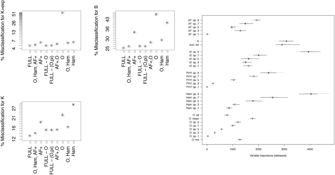
In Scenario 2, exponential growth and Beta coalescents are harder to distinguish. Again, adding statistics to the quantiles of the allele frequency spectrum helps distinguishing the model classes, see Figures 2-4. In Scenario 2, if the quantiles of the allele frequencies are used, we see, for n ≥ 100, that using AF+, O, Ham instead of the full set of statistics does not increase errors meaningfully (mean out-of-bag errors less than 0.2% apart in both replications), while taking all statistics but O has a stronger negative effect (mean out-of-bag errors increase by ≥ 1.5% compared to using AF+, O, Ham). For n = 25, this trend is considerably weaker, the full set of statistics has mean errors ≈ 0.6% lower than using AF+, O, Ham, and only leaving out O increases the error by 1% compared to AF+, O, Ham.

Classification errors of model comparison between 𝕂-exp and 𝔹 (Scenario 2) with n = 25. See Table 6 for the legend. The full set of statistics consists of r2,PHY, Ham, O,, S,π and either AF or SFS

Classification errors of model comparison between 𝕂-exp and 𝔹 (Scenario 2) with = 100. See Table 6 for the legend. The full set of statistics consists of r2, PHY, Ham, O,S, π and either AF or SFS

Classification errors of model comparison between 𝕂-exp and 𝔹 (Scenario 2) with = 200. See Table 6 for the legend. The full set of statistics consists of r2, PHY, Ham, O,S, π and either AF or SFS

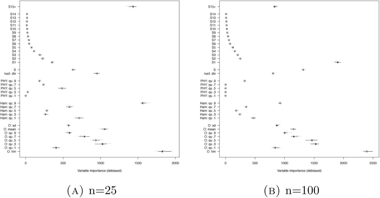
Variable importances for the model comparison between 𝕂-exp and 𝔹 (Scenario 2) using O, Ham, PHY, r2 and AF+. See Table 6 for the legend.
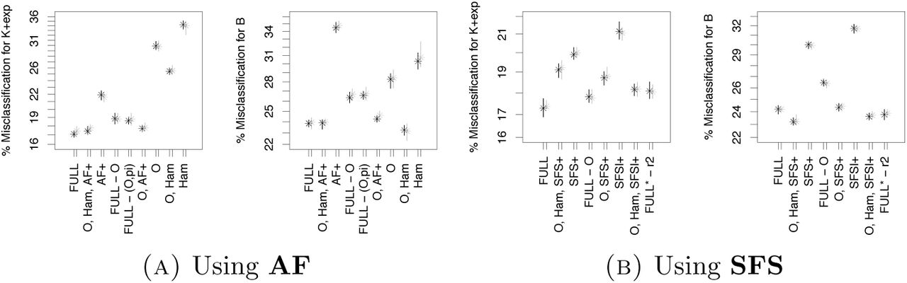
Using SFS instead of AF makes more information available, but also increases the number of statistics and likeley includes many weakly informative statistics. We first look at the classification errors in Figures 2 and 3. We see a strong effect that using SFS alone is clearly better than using AF alone (mean out-of-bag error difference ≥3%), but when coupled with other statistics, this effect vanishes. When using the full SFS, we see even a very slight increase of error for the full set of statistics or AF/SFS coupled with O and Ham, but this is vanishing when using the lumped SFS. We also see that the variation in classification errors of different ABC runs is smaller when AF is used compared to when SFS is used, seen as the size of the error bars in Figures 2 and 3. However, this effect is less pronounced for large sample size. The variable importances in Figure 6 are reflecting nicely that among the SFS statistics, especially the singleton mutation count and the lumped tails distinguish well between the genealogy model classes, which is the idea behind the singleton-tail statistic of [Kos18].

Variable importances for the model comparison between 𝕂 - exp and 𝔹 (Scenario 2) using O, Ham, PHY and SFS1+. See Table 6 for the legend.
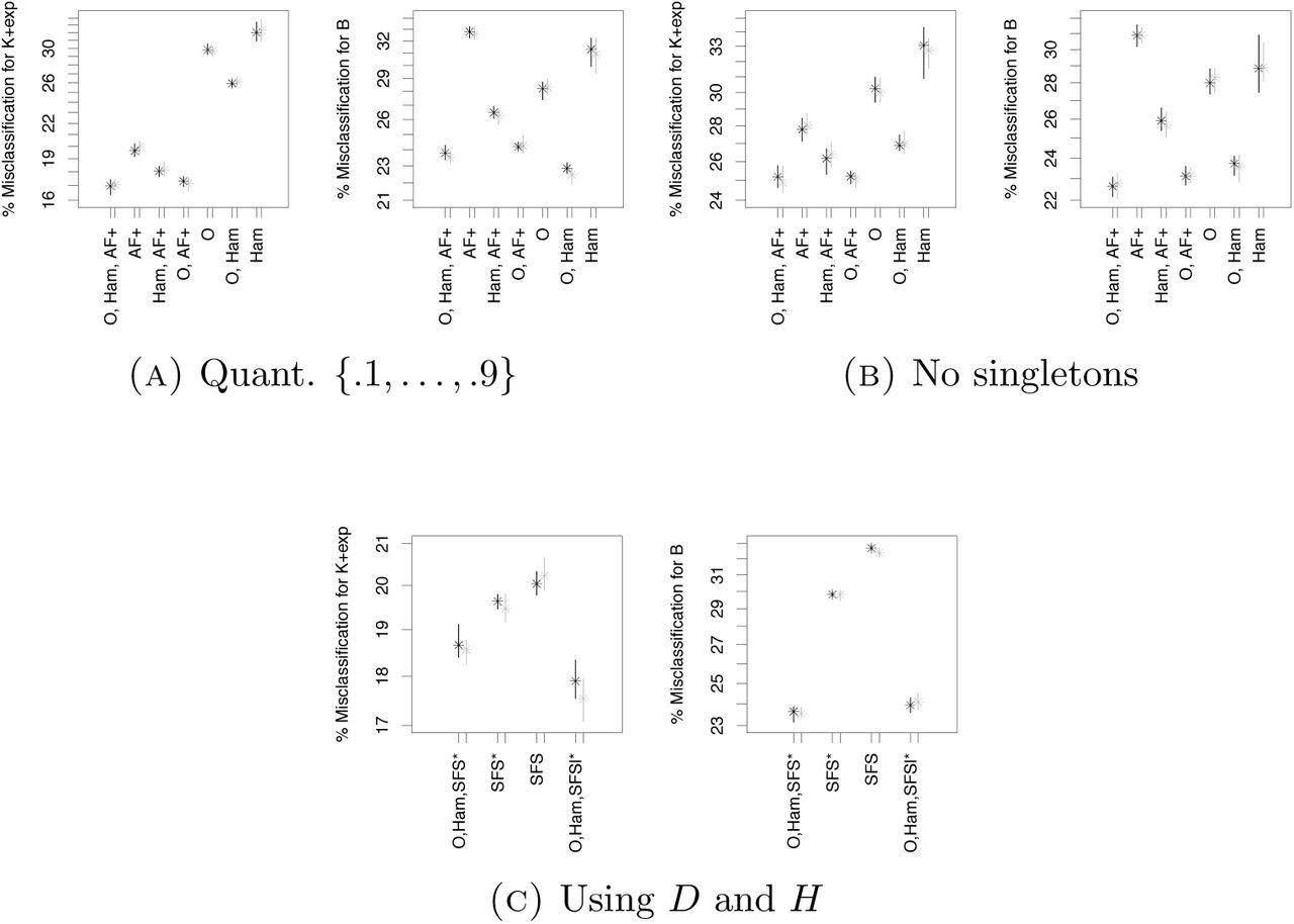
Since using the full SFS is not beneficial compared to using AF when combining with O, Ham, it is not surprising that using a finer mesh of quantiles for the statistics is not decreasing error rates meaningfully (mean out-of-bag error difference ≤0.5%), apart from a slight reduction of ≈2% mean out-of-bag error if only AF is used (see Figure 7(A)).
Classification errors of model comparison between 𝕂-exp and 𝔹 (Scenario 2) with n = 100. See Table 6 for the legend.

Classification errors of model comparison between 𝕂-exp and 𝔹- (Scenario 2) with n = 200. See Table 6 for the legend. The full set of statistics consists of r2, PHY, Ham, O, AF + and the (first and only) linear discriminant

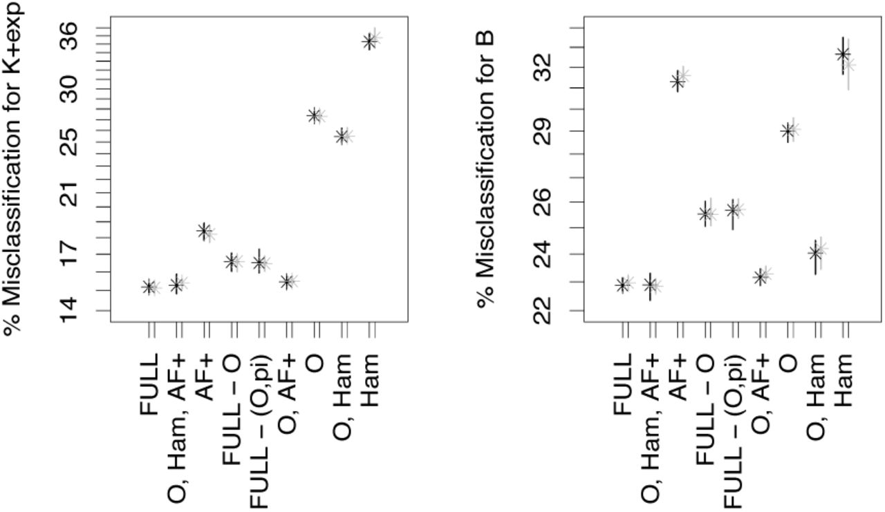
Classification errors and variable importances of model comparison between 𝕂-exp and 𝔹 (Scenario 2) with n = 100. See Table 6 for the legend. The full set of statistics consists of r2, PHY, Ham, O and fSFSI+
The considerable effect of O is only seen when used with other statistics, in all scenarios using O alone leads to strongly increased error rates. When coupled with other statistics though, O decreases error rates. In this situation, especially the harmonic mean of the minimal observable clade sizes is very helpful to distinguish between the hypotheses in Scenario 2, highlighted by it having highest importance score of all statistics, see Figures 5, 6 and 9. Additionally, O does not take into account singleton mutations. Consequently, we see that it stays a very beneficial addition to summary statistics if we ignore singleton mutations (e.g. if we are worried that they may be sequencing errors), see Figure 7(B). However, in this case we still have a ≈3% increase of mean out-of-bag error due to ignoring the informative singleton mutations.
Naturally, highly informative summaries directly constructed from the simulations on which the random forest is based, e.g. linear discriminants, have even higher importance (Figure 8) than e.g. the harmonic mean from O. However, misclassification rates are not affected considerably by adding the linear discriminant (changes in mean out-of-bag error below 0.5%). The latter is also true when specific SFS-based summaries to detect deviations from Kingman’s n-coalescent as Tajima’s D or Fay and Wu’s H are added, compare Figure 7(C) and 3(B): While there is a clear error reduction when only combined with the SFS, this vanishes when combined with the information from O and Ham (mean out-of-bag error difference of ≤0.2% in the latter case). This is also reflected by low variable importance of D and H, see Figure A13.
So far, we assume that one can polarize the data, i.e. that the ancestral and derived allele can be distinguished with certainty. However, this is usually done by comparison with one or more outgroups and is not error-free, see e.g. [KJ18]. Thus, this depends on the availability of suitable outgroups and may not always be possible or precise enough. If mutant and ancestral alleles cannot be distinguished, O cannot be computed and, for allele/site frequencies, one can only compute the folded site frequency spectrum fSFS (resp. the minor allele frequencies), while the other statistics S, π, PHY and r2 are still computable. In this case, while error rates are increased, there is still a clear benefit of adding statistics to the fSFS, see Figure 9. For instance, mean out-of-bag errors are reduced by 5% if one adds Ham and PHY to fSFS+. Again, as in the unfolded case, especially the information on the tail and the singletons is meaningful for the fSFS. In contrast to the unfolded case, adding r2 to the other statistics has a more than two-fold stronger effect than in the polarized scenario (mean out-of-bag error decrease of > 0.5%), while still being not overly strong. This stronger influence of r2 is also reflected in the variable importance estimates.
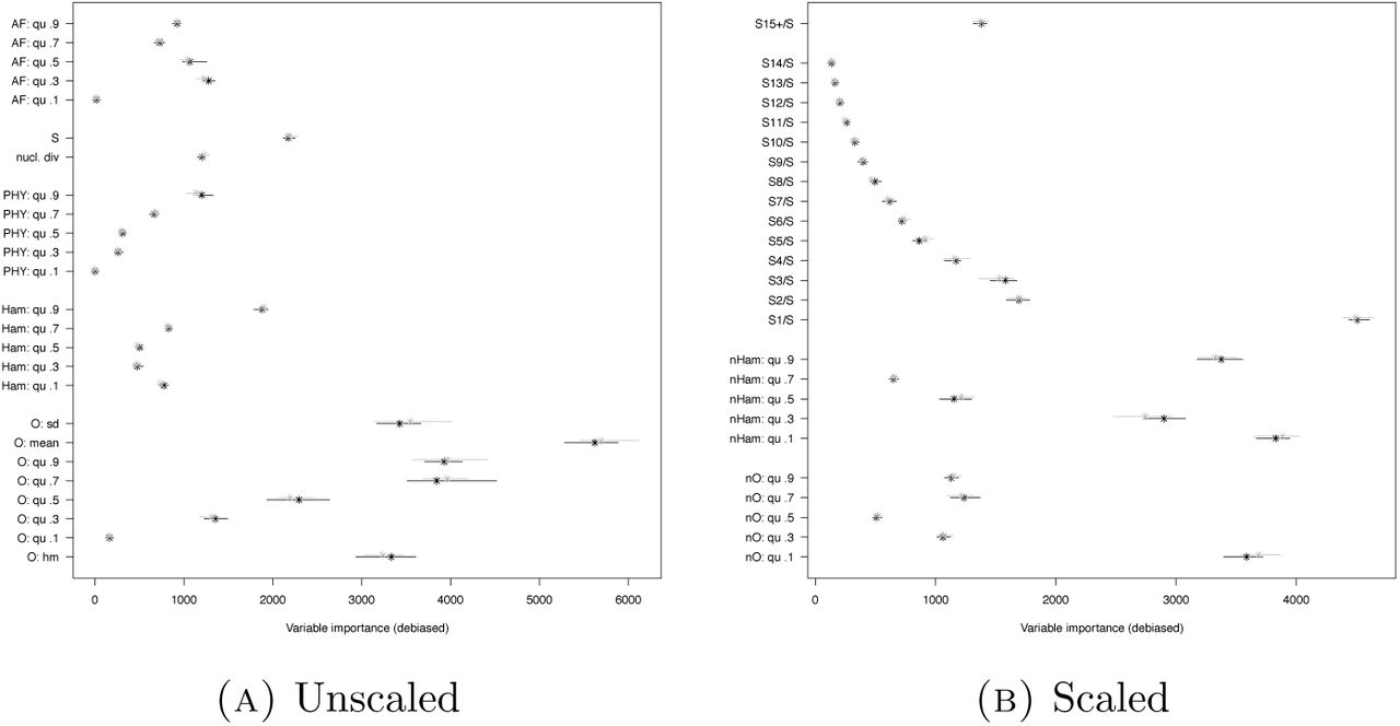
How realistic is Scenario 2? Bacteria species are often haploid species with a single-locus genome, neglectible amount of recombination, and potential for multiple mergers, due to rapid selection or quick emergence of specific strains. Here, we look at a scenario, which we denote by Scenario 3, matching a studied sample from Mycobacterium tuberculosis from [LRP+15] in sample size and number of mutations. Since the Watterson estimator  will be not estimating the true mutation rate perfectly, we allow θ to fluctuate around the Watterson estimate in the models, see Section 1.2. Due to the larger number of mutations expected, we left out the r2 statistics, since their number scales quadratically with the number of SNPs and thus pose a considerable computational burden. Misclassification is still common in Scenarios 1 and 2. In Scenario 3 however, classification errors drop considerably (mean out-of-bag error of 7.8-7.9% for O, Ham, AF+). Again, error rates without O, Ham are considerably higher, while using the full set O, Ham, AF+ and PHY has only a slight avantage over omitting PHY. For this scenario, we also checked whether adjusting the statistics O, Ham, SFS to be more robust towards changes in mutation rates helps for model class distinction. As discussed e.g. in [EBBF15], the scaled SFS nSFS is robust towards mutation rate changes. We also tried whether scaled versions of the other statistics decrease errors by being less prone for mutation rate dependent model class misclassifications. Being not influenced strongly by mutation rate changes works to a degree, though clearly less well than for the SFS, see Figures A2-A5. However, the information lost by scaling increases error rates, see Figure 10 (mean out-of-bag error ≈10.5% for nO, nHam, nSFS). However, adding the non-SFS statistics clearly reduces errors, so the chosen scaling of Ham and O does not make them uninformative for distinguishing model classes.

Classification errors and variable importances of model comparison between 𝕂-exp and 𝔹 (Scenario 3). See Table 6 for the legend. Full set of statistics in (A): PHY, Ham, O and AF+; in (B): nHam, nO and nSFSl
2.2 Comparison with Dirac and Beta-Ξ-n-coalescents
We consider again Scenario 2 with n = 100, where we subsequently add 𝔻 and 𝔻-exp. First, we perform model selection between all models, the results are shown in Figs. 12 and 13.


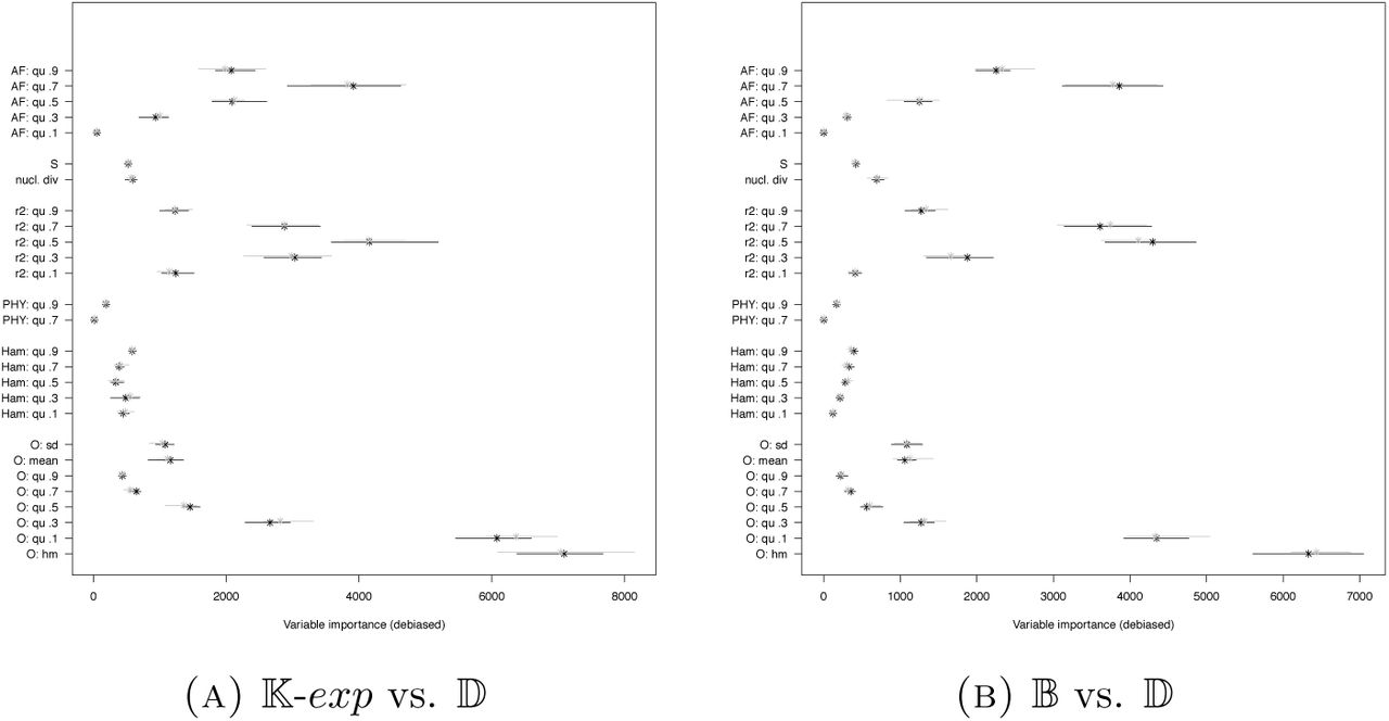
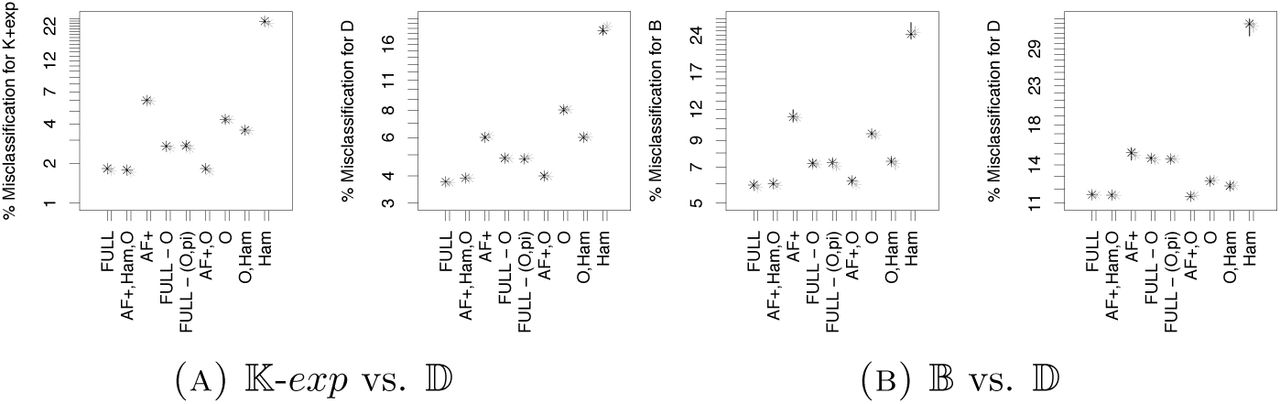
If we compare with the (pairwise) model selection between 𝕂-exp and 𝔹 (Figure 3), we see that adding 𝔻 leads to more frequent misidentification of 𝔹, but not of K-exp. The model class 𝔻 is easier to identify than the other two classes, having a far smaller misidentification probability. When we further add 𝔻-exp, we see that misidentification between 𝔻-exp and 𝔻 is quite common, while misidentification of 𝕂-exp and 𝔹 is essentially unchanged. Again, the variable with highest importance is the harmonic mean of the minimal observable clade sizes. How do model selection errors and variable importances change if we consider other pairwise model selections? We additionally performed model selection for 𝕂-exp vs. 𝔻 and for 𝔹 vs. 𝔻. The results are shown in Figures 14 and 15. The variable importances again are qualitatively similar, again the harmonic mean from O is the statistic with highest importance, followed by a group of statistics consisting of the quantiles of r2 (.5 and .7), AF (.7) and O (.1). As already known from earlier works, e.g. [EBBF15], the Dirac coalescent is easy to distinguish both from 𝕂-exp and 𝔹, reflected by the low misclassification rates compared to the model selection between 𝕂-exp and 𝔹.

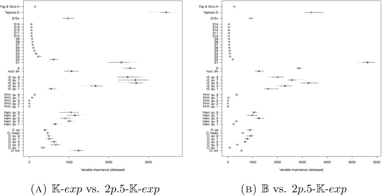
On the other hand, if we instead add Ξ-𝔹 as a model in Scenario 2, we see a strong increase in misclassification rates, see Figure 16. The high chance of misclassifying 𝔹 as Ξ-𝔹 stands out, see the results of the pairwise model selection approach in Figure 17. While for the three-fold comparison, the most important statistic still is the harmonic mean from O, followed by statistics from r2 and AF, this changes if one looks at the pairwise comparisons. There, O only plays an important, yet diminished role for distinguishing Ξ-𝔹 from 𝕂-exp, it seems to play much less of a role for distinguishing Ξ-𝔹 from 𝔹 (Figure 18). This is not entirely mirrored by the error rate changes between different sets of summary statistics, see Figure 17, but the differences between most sets of statistics for these scenarios are small to begin with.


Our results imply that the distribution of diversity statistics within different (parametric) subclasses of Ξ-n-coalescents can both be rather similar or very different. This also raises the question whether misspecifying the exact multiple merger model as a different multiple merger model increases model selection errors. We analyse this effect when the used reference model is 𝔹: We build a random forest from simulations of 𝔹 and 𝕂-exp, but perform model selection for simulations from the other multiple merger classes 𝔻and Ξ-B as described in Section A.2. The results are shown in Table 7. They highlight that multiple merger n-coalescents do not generally differ in the same way from 𝕂-exp. While 𝔻gets nearly always identified as 𝔹 instead of 𝕂-exp, this is not symmetric: 𝔹 gets slightly more often identified as 𝕂-exp. Unsurprisingly, given the high classification errors between 𝔹 and Ξ-𝔹, both models get more often identified as the other multiple merger model in contrast to as being identified as 𝕂-exp with chance slightly above 0.7. This means that if we use 𝔹 as a proxy model for Ξ-𝔹 and have to allocate a true realisation of Ξ-𝔹 to either 𝔹 or 𝕂-exp, this leads to considerably higher classification errors (though they should still be manageable) than for performing the model selection with the correct model Ξ-𝔹, see Figure 17. However, in this case only considering simulations that can be allocated to a model class with high posterior probability lowers errors, but at the cost of being unable to allocate a high proportion of observed data. To a degree, one can try to balance cost and benefit here, e.g. retaining only simulations from Ξ-𝔹 with posterior > 0.69 for either 𝔹 or 𝕂-exp, which is fulfilled by a proportion of 0.59 of simulations, leading to a decreased identification chance as 𝕂-exp of 0.18, which is comparable to the misidentification rate in the model selection using the correct model Ξ-𝔹.
→ B, → C: Proportion of simulations from model class allocated to two other model classes B,C in Scenarios 2 and 4. In parentheses: same proportion only among high posterior allocations. High posterior allocations are those with posterior probability > 0 9, the column ‘high posterior’ shows their proportion among all simulations from A. Random forest based on r2, PHY, Ham, Om AF+ for the first four rows r2, PHY, SFSl*, O and Ham for rows 5,6. Results are rounded to two digits.
2.3The influence of exponential growth
We further consider Scenario 5, focusing only on comparisons between scenarios with growth and without, see Figure 19. Even for 𝕂 vs. 𝕂-exp and high mutation counts, the model with growth is relatively often misidentified, which partly comes from our focus on low to medium growth rates, compared e.g. to [EBBF15]. For instance, subsetting for only growth rates above 20 (and drawing the same number of simulations from 𝕂) leads to a probability of < 1% to misidentify for both comparisons. Additionally, the larger error for identifying 𝕂-exp is also affected by the prior: we have only a relatively small number of simulations from models close to 𝕂 (i.e. with very small growth rates) which are very hard to distinguish from 𝕂. Such simulations, if left out of a bootstrap sample, then get easily sorted into a leaf associated to the more numerous simulations from 𝕂.

A fundamental change to the scenario of distinguishing multiple mergers from exponential growth is that the importance of statistics is changed. Here, r2 and the allelic spectrum are among the most important statistics, while the observable clade sizes and the Hamming distances score relatively low.
If one looks at distinguishing 𝔻 from 𝔻-exp, now again with the lower mutation rates of Scenario 2, we see increased error probabilities. While 𝔻 could be well distinguished from 𝔹 and 𝕂-exp, see Figure 14, it is much more similar in its summary statistics to 𝔻-exp. Again, O is not useful to distinguish 𝔻 from 𝔻-exp, the two most important statistics come from the set r2.

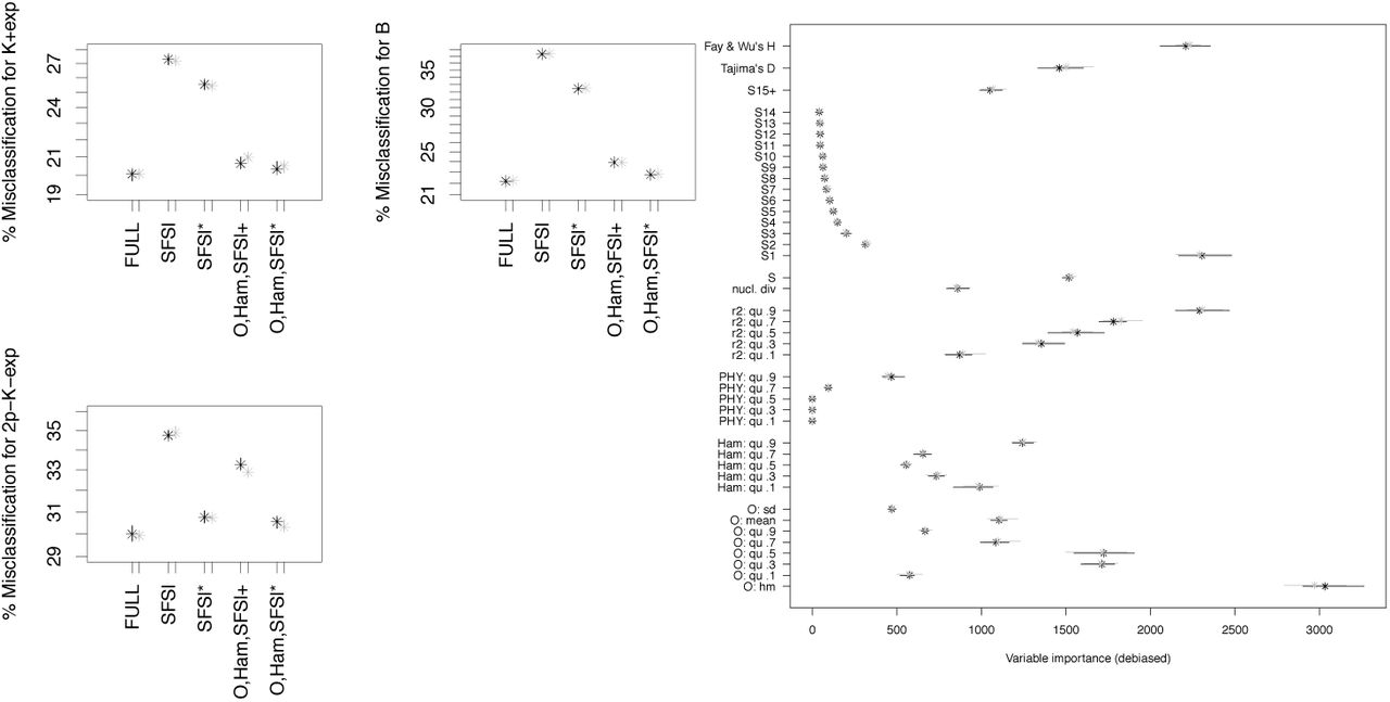
2.4 The influence of population structure
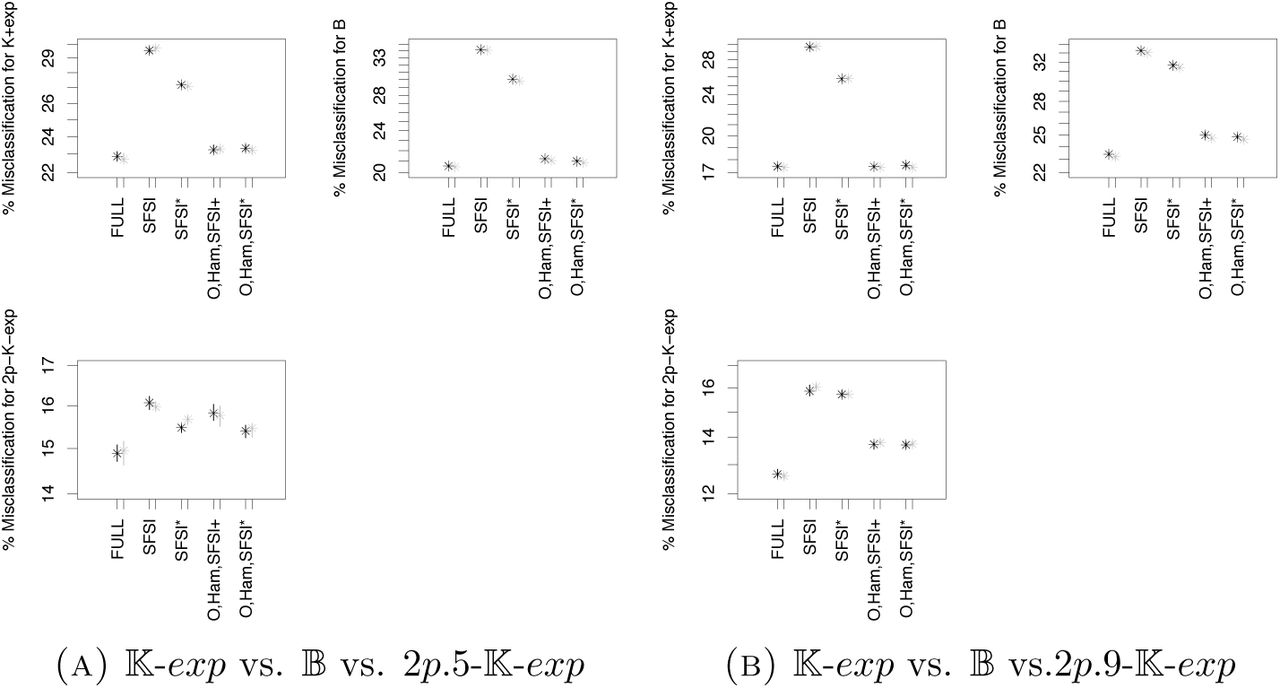
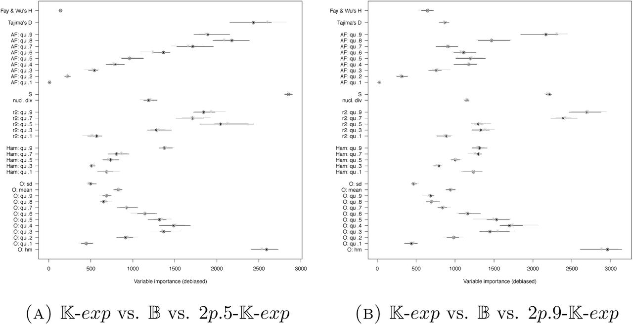
For two very simplistic scenarios with two subpopulations and low symmetric migration rates, where either equal samples or skewed samples are taken from the subpopulations, we find that model classes 𝕂-exp, 𝔹 and 2p5/2p9-𝕂-exp with population structure can be distinguished quite well compared to other sets of models. As statistics, we use the SFS lumped at a mutant allele count of 15, π, S, Tajima’s D, Fay and Wu’s H, the (.1, .3, .5, .7, .9) quantiles of O, Ham, PHY and r2 (D, H were added due to their known potential to distinguish demography from population structure). Again, adding non-SFS based statistics is rather beneficial. For the three-wise model comparison, see Figure 21, already adding the further SFS-based statistics π, S, Tajima’s D and Fay and Wu’s H decreases errors (reduction of mean out-of-bag error of ≈2%), while adding O and Ham reduces this even more strongly (further mean out-of-bag error reduction ≥4%, ≥5.5% for the model selection with class 2p5– 𝕂-exp, 2p9-𝕂-exp). Further adding of PHY and r2 as summary statistics does not decrease the errors strongly (between .5-1% reduction). This is also partly reflected in the variable importance scores, see Figure 22. While the singleton signal S1 and the harmonic mean of O are always among the most important statistics, and some quantiles of r2 have comparably high importance, for equal subsample sizes Tajima’s D is highly relevant only in the case of equal sampling from the subpopulations. While the error rates strongly drop for pairwise comparisons between model classes (Figures 23,A10), at least for the misidentification probabilities the qualitative picture remains: an error drop-off when adding Ham and O, while further adding PHY and r2 leads to a further decrease (the second decrease appears to be somewhat stronger relative to the first then in the three-wise model selection). However, there is a slightly surprising change when looking at variable importances (Figures 24, A11): no statistic of O is under the most important statistics, while the count S1 of singleton mutations and Tajima’s D are among the statistics with high importance (the latter only for equally sized subsamples).
Classification errors in Scenario 4, n = 100. See Table 6 for the legend. Full set of statistics includes r2, PHY, SFSI*, O and Ham.

Variable importances in Scenario 4, n = 100. See Table 6 for the legend.

Classification errors for model selection in Scenario 4, n = 100. See Table 6 for the legend. Full set of statistics includes r2, PHY, SFSI*, O and Ham.

Variable importances in Scenario 4, n = 100. See Table 6 for the legend.
Another facet of this inference problem is whether lumping the SFS increases error rates due to mixing intermediate and high mutant allele frequencies. We analyzed this by replacing the lumped SFS as summary statistics with a fine mesh of quantiles of the unlumped SFS. The results are shown in Figures A8 and A9. They show that no lumping indeed leads to a slight reduction in error, most notably when sampling 90% of the sample from a single subpopulation (mean out-of-bag error decrease of ≈1% for equal-size sampling when using quantiles of the SFS instead of the lumped SFS, while always adding standard SFS-related statistics D, H, S, π). This effect gets further weakened if we use summary statistics beyond the site frequency spectrum. The slight reduction is also reflected by the variable importances shown in Figure A9: high quantiles of the allele frequencies show intermediate to large importance scores, relative to the other statistics.
While the simple scenario of strong population structure and two subpopulations can be quite well distinguished from 𝕂-exp and 𝔹, this only works when population structure is known a priori. Indeed, if we allocate simulations from 2p.5-𝕂-exp to 𝕂-exp or 𝔹, i.e. perform model selection between the latter two models based on data that truly follows 2p.5-𝕂-exp, Table 7 reveals that these simulations are just randomly assigned to one of the model classes. To be allowed to ignore population structure for inference, such simulations should be sorted into 𝕂-exp with high probability, which is clearly not the case. Even worse, if we just focus on those simulations that are allocated to one model class with high posterior probability, there is a higher chance to be falsely associated with a multiple merger model. This bias towards identifying population structure as multiple mergers shows both for all allocated simulations or only those allocated with high confidence if we consider Scenario 4 when sampling the majority of individuals from one subpopulation.
3. Discussion
Our results highlight that the information not contained in the site frequency spectrum is still valuable for distinguishing between different classes of n-coalescents, e.g. between exponential growth and multiple merger coalescents. In addition to scenarios with fixed mutation rate ranges across models as in [KVS+17], this also holds true for scenarios where mutation rates are chosen so that, on average, each model produces the same number of mutations. The benefit of including statistics not based on the SFS is especially relevant for species with small genomes and few unlinked loci, e.g. for many bacterial species, but also likely for some selfing plants and clonally propagating fungi. Giving high enough mutation rates and reasonable sample sizes, as in our Scenario 3, one can distinguish exponential growth from multiple mergers with ease. We emphasize that seeing hundreds of mutations at a single locus in a species with low recombination rates is not unrealistic (though clearly not always the case), we based our setting on real data sets in Mycobacterium tuberculosis. While model misidentification becomes less of an issue if the genome consists of many unlinked loci, see [Kos18], this may still be relevant if further evolutionary processes are acting, as discussed in [KWB19].
The computational burden of obtaining statistics can be considerable. Usually, one has many more SNPs than individuals, thus punishing more strongly statistics that scale with the number of mutations, most notably r2. We thus focused on assessing the effect of adding the two most computationally expensive sets of statistics, r2 and PHY, to all other statistics. This effect is beneficial but very small if the SFS is summarized by AF apart from the threefold model comparison between Kingman’s n-coalescent with exponential growth, the same model with strong population structure and Beta-coalescents. Additionally, the information within the SFS (and within the Hamming distances and minimal observable clade sizes) to distinguish the model classes seems to be already contained in a coarse summary of its shape if it is combined with other statistics, i.e. already 5 quantiles of the allele frequencies allow model selection with comparable errors as a finer mesh of quantiles. Using the full SFS also may increase error rates or at least increase variability between ABC runs, likely due to the inclusion of many more weakly informative summary statistics. Thus, our results suggest that using a statistical approach based on quantiles (.1, .3, .5, .7, .9) of the allele frequency spectrum, standard diversity measures S and π as well as the same quantiles of the Hamming distances and of the minimal observable clade sizes are a reasonable compromise of extracting as much information from the data as necessary for low misidentification rates, but maintaining feasible computation times. However, the computational burden of statistical approaches strongly depend on the implementation of the approaches and its significance on the resources at hand. Nevertheless, our results can be seen as emphasizing the importance of finding statistical methods based on extracting only relevant features of the data for distinguishing between genealogy models, e.g. as done in [PVC+19], to decrease computational costs. While we have included a wide range of non-SFS-based statistics of genetic diversity, further interesting statistics to add to the SFS are available, most notably including linkage information via the two-site frequency spectrum as in [RND18].
Compared with the results in [KVS+17], our results show highly increased error rates. This is likely not a consequence of our ABC approach, but of our focus on distinguishing Beta(2 – α,α)-n-coalescents for α ∈ [1, 2) from Kingman’s n-coalescent with growth, while [KVS+17] also add further Beta coalescents that are easier to distinguish from the bifurcating genealogies. Nevertheless, this specific set of Beta(2 – α,α)-n-coalescents is chosen in this study because it arises as limit genealogies of mathematical evolutionary models [Sch03].
As reported in [KWB19], considering Kingman’s n-coalescent with both exponential growth and population structure often causes dramatic misidentification of whether multiple merger coalescents are the correct genealogy models or not. Our results confirm that this is not only a consequence of the use of the singletons and the tail of the site frequency spectrum. Even when adding non SFS-based statistics, non-accounted population structure makes correct inference of multiple merger genealogies essentially impossible. For data sets containing many unlinked loci, assessing population structure may be, at least approximately, possible with standard model-free methods like DAPC [JDB10] or principal component analysis. On the plus side, both our results and the results from [KWB19] show that the genetic diversity between model classes with and without population structure (and multiple mergers) is different enough so that additional population structure should be detectable, the open question is how to do it. One potential avenue based on the ABC with random forest approach would be to not estimate population structure at all, but instead to include a further model class that combines Kingman’s n-coalescent with exponential growth and not one specific model of population structure but the complete range of reasonable populations structure setups. We did this in very limited fashion for populations with two subpopulations of equal size, variable migration rates and subsample sizes, see Section A.5. At least in this scenario, Table A2 shows that Kingman’s n-coalescent with exponential growth, Beta-n-coalescents or Kingman’s n-coalescent with exponential growth and specific models of population structure can be allocated to the true model class with much lower error rates than when just allocating to the models without accounting for population structure. This works both for adding population structure with parameters already featuring in the model class used for training the random forest or not, and does not need a precise a priori knowledge or independent estimation of the population structure.
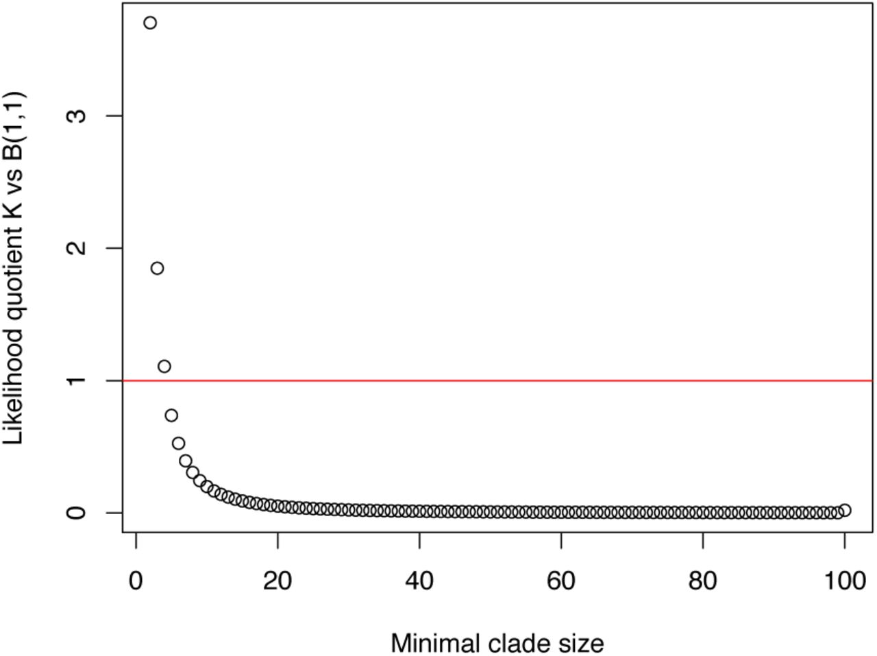
We introduced a new statistic, the minimal observable clade size, defined in Equation (1). This statistic, for a non-recombining locus, gives the clade size of the smallest genealogical clade each individual is a member of, and that can be distinguished from data, see Section A.1. It is not very costly to compute, its computational cost scales well with both population size and mutation rate (see Table A1) and, for most scenarios, decreases error rates considerably if (and only if) coupled with other summary statistics. While it needs polarized data, i.e. one needs to be able to tell apart ancestral and derived states of segregating sites, it is not taking into account any single-ton mutations, which makes it relatively robust towards sequencing errors, see [Ach08]. Intuitively, the statistic should be suited well for distinguishing between multiple merger genealogies and Kingman’s n-coalescent with population size since it is an upper bound of the size of the minimal clade, i.e. the size of the clade spanned by the most recent ancestor node in the genealogy of each individual. For high enough mutation rates, the minimal observable clade size should equal it or be close to it. The minimal clade is known to be typically small for Kingman’s n-coalescent, while larger for Beta-n-coalescents, see [BF05], [FSJ14] and [SJY16] and Figure A1 for an example. Additionally, it is by definition invariant under population size changes which result in just a rescaling of coalescent times. That the latter translates to a weak effect of population size changes on the observable minimal clade sizes is suggested by our results. The harmonic mean of all minimal observable clade sizes often shows one of the highest variable importance among all statistics. A heuristic argument for this is that some of the minimal observable clades may be also minimal clades (i.e. if there is a mutation on the branch adjacent to the ancestor of the minimal clade on its path to the root of the genealogy), thus inheriting the potential of the minimal clade to distinguish between coalescent models. Additionally, not only the information about small clades is included, which may prove beneficial, since the minimal observable clade, at least for large n and θ, should for many models be 2. For Kingman’s n-coalescent, this is clear from [DK15] and for Beta coalescents from [BBL14, Thm. 8].
FF was funded by DFG grant FR 3633/2-1 through Priority Program 1590: Probabilistic Structures in Evolution. The authors acknowledge support by the state of Baden-Württemberg through bwHPC.
Appendix A. Supplementary information
A.1 The minimal observable clade [FSJ19]
Consider any (genealogical) tree with n leaves with s mutations on its branches interpreted under the infinite sites model. A clade of the genealogy is a set of leaves that have a common ancestor. Consider all clades that include i. In a tree, these need to be nested. Any mutation describes a clade in the tree, the set of all sequences sharing this mutation. A clade can only be distinguished from the SNP matrix if there is a mutation directly on the branch connecting the ancestor of the clade to the rest of the tree in direction towards the root. Implicitly, this requires that we can distinguish the mutation from the ancestral type. Each non-private mutation of individual i, i.e. which appears in i and at least one other individual, which has the minimal allele count among all mutations of i, defines the same clade, the minimal observable clade of i. Since the minimal clade of i is the smallest clade containing i, it has to be nested within the minimal observable clade of i. Thus, the size M (i) of the minimal clade satisfies M (i) ≤ O(i). The minimal observable clade is the minimal clade (M (i) = O(i)) if and only if there is one or more mutations on the branch connecting the ancestor of the minimal clade to the root of the genealogy. The minimal clade does only depend on the tree topolgy, not on the branch lengths, so it is invariant for any population size changes that only lead to a time-change of the genealogical tree, see e.g. [Fre19] for a discussion. The minimal clade is only observable in the data if it equals the observable clade.

Likelihood ratios for the minimal clade size between Kingman’s 100-coalescent and the Bolthausen-Sznitman 100-coalescent
The distribution of the minimal clade size of an individual i is known for fixed sample size n for both Kingman’s n-coalescent [BF05] and the Bolthausen-Sznitman n-coalescent 𝔹 with parameter α = 1 [FSJ14]. Thus, we can compute exact likelihood ratios, which we show for n = 100 in Figure A1.
A.2 Model selection for observed/pseudo-observed data
Given a random forest trained to distinguish between model classes, the approach from [PME+15] performs model selection for a set of observed summary statistics by a majority vote: The model that the data is allocated to by the decision trees in the (simple) majority of cases is the selected one. A second approach from [PME+15] also allows to give an estimate of the posterior probability for this choice of model M : First, for each simulation, the (out-of-bag) misclassifier  from the majority vote all trees built without them, i.e. 0 if the majority vote is model M and 1 otherwise, is recorded. Then, a second random forest from the same simulations is trained to perform a regression of these values
  on the summary statistics, i.e. to predict
  using a random forest of decision trees on the summary statistics (the trees are built slightly different as for model selection, see [PME+15] for details), the estimate is then the average over the forest. Then, for the actual observed summary statistic, the posterior probability of classifying as M is reported as the average estimate of
  over the second random forest.
We apply this approach in sets of simulations from three model classes. The simulations from one model class are treated as (pseudo-)observed data: For each simulation, the best fitting model class from the remaining model classes is recorded (so the winner of the majority vote), alongside its posterior probability. In this case, we build all random forests from the full set of statistics in the scenario.
A.3 Computation times for summary statistics
We measured the time necessary to compute 1,000 simulations for 𝕂-exp and B in 3 scenarios (with ten replications): Scenario 2, Scenario 3 with mutation rate θ fixed as the generalized Watterson estimate for each model parameter choice and a new scenarion which is as Scenario 3, but with increased sample size n = 500 and increased mutation rates given by the Watterson estimate based on s = 500 mutations assumed to be observed. This scenario is referred to as Scenario 3+. The computation times are given for our implementation of the statistics (code currently available on request, but will be soon put in a public repository). Times were measured via the R commmand system.time and the total elapsed time is reported. For all sets, quantiles (.1, .3, .5, .7, .9) were used. Due to long running times, we employed parallelisation when computing r2.
Range [min max] of computation times for 1000 simulations in seconds for different sets of summary statistics across 10 replications
A.4 Simulations of robust statistics
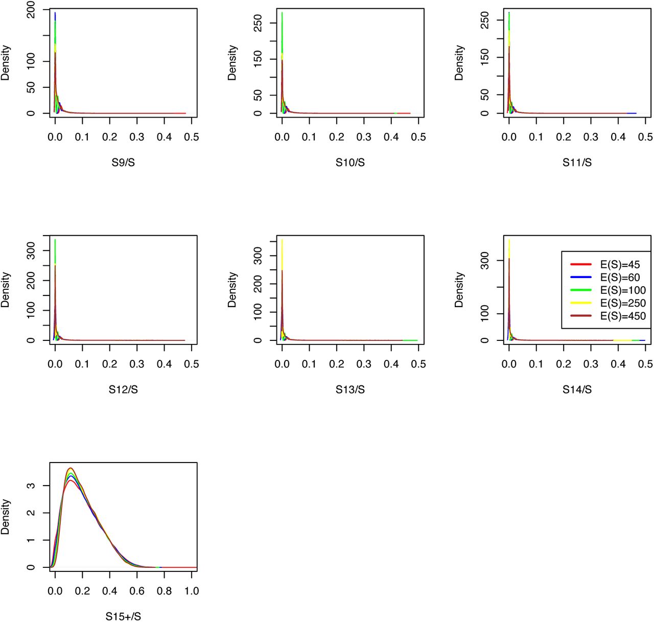
We used the simulation scheme for Scenario 3 for model classes 𝕂-exp and for 350,000 simulations, apart from setting the mutation rates to the Watterson estimator on assumed counts of s ∈ {45, 60, 100, 250, 450} mutations in the sample, endowed with an uniform prior. We simulated the sets nSFS, nHam and nO of statistics. Figures A2 to A7 show kernel density estimates of their distributions.
A.5 Using a priori arbitrary structured populations to assess multiple mergers vs. exponential growth in structured populations
Assume Scenario 4 with n = 100, but replace the fixed migration rate as well as the fixed subsample sizes with scaled migration rates m picked uniformly from {0.1, 0.6, … ., 2.1} and subsample sizes picked uniformly from {(10, 90), (20, 80), (30, 70), (60, 40), (50, 50)}. We used the same summary statistics as in the analysis for Scenario 4 in Section 2.4. We generated 175,000 simulations under each scenario twice. Figure A12 shows the result of the three-fold model selection in this scenario, where we denote the model class with population structure and growth by 2p-𝕂-exp. We then took the random forest trained on the first 175,000 simulations and allocated the set of simulations for model classes 2p.5-𝕂-exp and 2p.9-𝕂-exp using ABC based on the constructed random forest and recorded the proportion of misclassification for all simulations and for the ones allocated with high posterior probability as described in Secyion A.2. We then generated a third set of simulations, where we changed migration rates to be uniformly picked from {0.5, 1} and subsample sizes from (5, 95), (25, 75), (45, 55). For these simulations, we denote the model class with population structure and growth by 2p*-𝕂-exp. We used the random forest constructed above, allocated also these simulations and recorded the errors as for the second set of simulations. Results are summarized in Table A2.

Distributions of statistics nO and nHam in a modified Scenario 3 for𝕂-exp

Distributions of statistics nHam and nSFS in a modified Scenario 3 for 𝕂-exp
A.6 Comparison with other ABC approaches
For Scenario 1 and for Scenario 2 with n = 100 and model classes 𝕂-exp, 𝔹 and 𝔻, we performed ABC model selection. We used O, Ham, PHY, r2, AF+ as summary statistics with quantiles (.1, .3, …, .9). We compared the ABC with random forest as described in the main manuscript with three standard ABC approaches as implemented in the R package abc: the simple rejection method (REJ), using multinomial logistic regression (MNL) and the neural net approach (NN). For the latter three methods, we used a strict tolerance level of 0.002. All four methods were based on 175,000 simulations per model class as described in the main manuscript.
To assess errors, we then performed model selection for an independent test set of 500 simulations per model class that then was allocated to the three model classes. For the random forest approach, we proceeded as described in Section A.2, for the other methods we set the model selected to the model with the highest posterior probability. Misclassification is reported in Table A3. In Scenario 2, there seems to be a criterion shift for ABC methods NN and MNL, leading to a decrease of misclassification for 𝔹 and an increase of error for 𝕂-exp. However, the average error is considerably higher than for RF (even when ignoring 𝔻).

→, →: Proportion of simulations from model class A allocated to two other model classes B,C in Scenarios 2 and 4. In parentheses: same proportion only among high posterior allocations. HP: High posterior allocations are those with posterior probability > 0:9, the column ‘high posterior’ shows their proportion among all simulations from A. Random forest based on summary statistics r2, PHY, SFSl*, O and Ham Results are rounded to two digits.


Misclassification frequencies of 500 simulations/model based on 175,000 simulations per model class. ABCs based on MNL=multinomial logistic regression, NN=Neural net, REJ = rejection, RF = random forests.

Classification errors for model selection in Scenario 4, = 100. See Table 6 for the legend. Full set of statistics includes r2, PHY, AF*, O and Ham


Classification errors for model selection in Scenario 4, = 100. See Table 6 for the legend. Full set of statistics includes r2, PHY, SFSl*, O and Ham.

Classification errors and variable importances for model selection 𝕂-exp vs. 𝔹 vs. 2 -𝕂-exp (variable migration rates and subsample sizes) in Scenario 4 (n = 100). See Table 6 for the legend. Full set of statistics includes r2, PHY, SFSl*, O and Ham.

Variable importances for model selection 𝕂-exp vs. 𝔹 in Scenario 2 (n = 100). See Table 6 for the legend.
References
- [Ach08].↵
- [BBL14].↵
- [BCEH16].↵
- [BF05].↵
- [BLS18].↵
- [CB17].↵
- [Che11].↵
- [DK15].↵
- [DS05].↵
- [DWF13].↵
- [EBBF15].↵
- [EW06].↵
- [Fre19].↵
- [FSJ14].↵
- [FSJ19].↵
- [FW00].↵
- [GCMPSJ19].↵
- [GT94].↵
- [HSJB19].↵
- [ILM+16].↵
- [JDB10].↵
- [KJ18].↵
- [Kos18].↵
- [KVS+17].↵
- [KWB19].↵
- [LRP+15].↵
- [MHAJ18].↵
- [Möh98].↵
- [Möh06].
- [MS01].↵
- [NH13].↵
- [NNY16].↵
- [Pit99].↵
- [PME+15].↵
- [PVC+19].↵
- [RND18].↵
- [SBB13].↵
- [SBZH07].↵
- [Sch00].↵
- [Sch03].↵
- [Sch17].↵
- [SJY16].↵
- [Ste09].↵
- [SZ08].↵
- [Taj89].↵
- [TL14].↵
- [WH98].↵
- [WZ17].↵


