

Abstract
Many biotic and abiotic factors that influence the distribution, abundance, and diversification of species can simultaneously affect multiple evolutionary lineages within or across communities. These include environmental changes and inter-specific ecological interactions that cause ranges of multiple, co-distributed species to contract, expand, or become fragmented. Such processes predict temporally clustered patterns of evolutionary events across species, such as synchronous population divergences and/or changes in population size. This has generated interest in developing statistical methods that infer such patterns from genetic data. There have been a number of methods developed to infer shared divergences or changes in effective population size, but not both, and the latter has been limited to approximate Bayesian computation (ABC). We introduce a general, full-likelihood Bayesian method that can estimate temporal clustering of an arbitrary mix of population divergences and population-size changes across taxa. We use this method to assess how well we can infer temporal patterns of shared population-size changes compared to divergences when using all the information in genomic data. We find that estimating the timing and sharing of demographic changes is much more challenging than divergences. Even under favorable simulation conditions, the ability to infer shared demographic events is quite limited and very sensitive to prior assumptions, which is in sharp contrast to accurate, precise, and robust estimates of shared divergence times. Our results also suggest that previous estimates of co-expansion among five Alaskan populations of threespine sticklebacks (Gasterosteus aculeatus) were likely spurious, and driven by a combination of mispecified prior assumptions and the lack of information about the timing of demographic changes when invariant charcters are ignored. We conclude by discussing potential avenues to improve the estimation of synchronous demographic changes across populations.
1 Introduction
A primary goal of ecology and evolutionary biology is to understand the processes influencing the distribution, abundance, and diversification of species. Many biotic and abiotic factors that shape the distribution of biodiversity across a landscape are expected to affect multiple species. Abiotic mechanisms include changes to the environment that can cause co-distributed species to contract or expand their ranges and/or become fragmented (Wegener, 1966; Avise et al., 1987; Knowles and Maddison, 2002). Biotic factors include inter-specific ecological interactions such as the range expansion of a species causing the expansion of its symbionts and the range contraction and/or fragmentation of its competitors (Lotka, 1920; Volterra, 1926). Such processes predict that evolutionary events, such as population divergences or demographic changes, will be temporally clustered across multiple species. As a result, statistical methods that infer such patterns from genetic data allow ecologists and evolutionary biologists to test hypotheses about such processes operating at or above the scale of communities of species.
Recent research has developed methods to infer patterns of temporally clustered (or “shared”) evolutionary events, including shared divergence times among pairs of populations (Hickerson et al., 2006, 2007; Huang et al., 2011; Oaks, 2014, 2019) and shared demographic changes in effective population size across populations (Chan et al., 2014; Xue and Hickerson, 2015; Burbrink et al., 2016; Xue and Hickerson, 2017; Gehara et al., 2017) from comparative genetic data. To date, no method has allowed the joint inference of both shared divergences and demographic changes. Given overlap among processes that can potentially cause divergence and demographic changes of populations across multiple species, such a method would be useful for testing hypotheses about community-scale processes that shape biodiversity across landscapes. Here, we introduce a general, full-likelihood Bayesian method that can estimate shared times among an arbitrary mix of population divergences and population size changes (Figure 1).
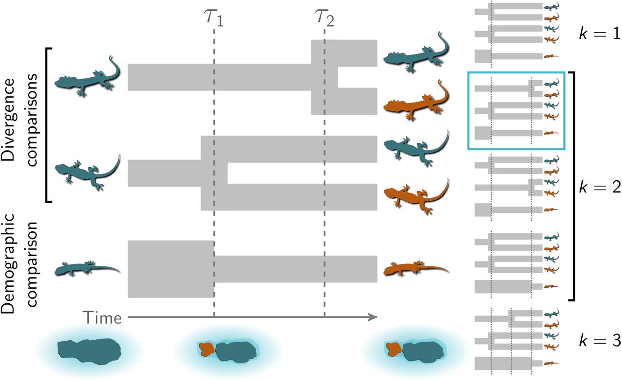
An illustration of the general phylogeographic model using three insular lizard taxa. The top two comparisons are pairs of populations for which we are interested in comparing their time of divergence (“divergence comparisons”). The bottom comparison is a single population for which we are interested in comparing the time of population-size change (“demographic comparison”). In this scenario, three species of lizards co-occured on an island that was fragmented by a rise in sea levels at time τ1. Due to the fragmentation, the second lineage (from the top) diverged into two descendant populations while the population size of the third lineage was reduced. The first lineage diverged later at τ2 due to another mechanism, such as over-water dispersal. The five possible event models are shown to the right, with the correct model indicated. The lizard silhouette for the middle pair is from pixabay.com, and the other two are from phylopic.org; all were licensed under the Creative Commons (CC0) 1.0 Universal Public Domain Dedication. Modified from Oaks (2019).
Whereas the theory and performance of methods that estimate shared divergence times has been relatively well-investigated (e.g., Oaks et al., 2013; Hickerson et al., 2014; Oaks et al., 2014; Oaks, 2014; Overcast et al., 2017; Oaks, 2019), exploration into the estimation of shared demographic changes has been much more limited. There are theoretical reasons to suspect that estimating shared demographic changes is more difficult than divergence times. The parameter of interest (timing of a demographic change) is informed by differing rates at which sampled copies of a gene “find” their common ancestors going backward in time (coalescence) before and after the change in population size, and this can become unidentifiable in three ways. First, as the magnitude of a change in population becomes smaller, it becomes more difficult to estimate. Second, as the age of the demographic change gets older, fewer of the genetic coalescent events occur prior to the change, resulting in less information about the timing and magnitude of the change. Third, as the age of the demographic change approaches zero, fewer coalescent events occur after the change, again limiting information about the timing and magnitude of the change. Thus, we take advantage of our full-likelihood method to assess how well we can infer shared demographic changes among populations when using all the information in genomic data. We apply our method to restriction-site-associated DNA sequence (RADseq) data from five populations of three-spine stickleback ((Gasterosteus aculeatus); Hohenlohe et al., 2010) that were previously estimated to have co-expanded with an approximate Bayesian computation (ABC) approach (Xue and Hickerson, 2015).
2 Materials & Methods
2.1 The model
We extended the software package, ecoevolity, to accommodate two types of temporal comparisons:
A population that experienced a change from effective population size
 to effective size at time t in the past. We will refer to this as a demographic comparison (Figure 1), and refer to the population before and after the change in population size as “ancestral” and “descendant”, respectively.
A population that diverged at time t in the past into two descendant populations, each with unique effective population sizes. We will refer to this as a divergence comparison (Figure 1).


This allowed us to infer shared times of divergence and/or demographic change across an arbitrary mix of demographic and divergence comparisons in a full-likelihood, Bayesian frame-work. During an “event” at time τ, one or more demographic changes and/or divergences can occur. We estimate the number and timing of events and the assignment of comparisons to those events under a Dirichlet-process (Ferguson, 1973; Antoniak, 1974) prior model. The a priori tendency for comparisons to share events is controlled by the concentration parameter (α) of the Dirichlet process. We use Markov chain Monte Carlo (MCMC) algorithms (Metropolis et al., 1953; Hastings, 1970; Neal, 2000) to sample from the joint posterior of the model. See Appendix A for a full description of the model, and Table 1 for a key to the notation we use throughout this paper.
2.2 Software implementation
The C++ source code for ecoevolity is freely available from https://github.com/phyletica/ecoevolity and includes an extensive test suite. Documentation for how to install and use the software is available at http://phyletica.org/ecoevolity/. We have incorporated help in pre-processing data and post-processing posterior samples collected by ecoevolity in the Python package pycoevolity, which is available at https://github.com/phyletica/pycoevolity. We used Version 0.3.1 (Commit 9284417) of the ecoevolity software package for all of our analyses. A detailed history of this project, including all of the data and scripts needed to produce our results, is available at https://github.com/phyletica/ecoevolity-demog-experiments.
2.3 Analyses of simulated data
2.3.1 Assessing ability to estimate timing and sharing of demographic changes
We used the simcoevolity and ecoevolity tools within the ecoevolity software package to simulate and analyze data sets, respectively, under a variety of conditions. Each simulated data set comprised 500,000 characters collected from 10 diploid individuals (20 genomes) sampled per population from each of three demographic comparisons. We specified the concentration parameter of the Dirichlet process so that the mean number of events was 2 (α = 1.414216). We assumed the mutation rate of all three populations was equal and 1, such that time and effective population sizes were scaled by the mutation rate. When analyzing each simulated data set, we ran four MCMC chains run for 75,000 generations with a sample taken every 50 generations; we combined and summarized the last 1000 samples of each of the four chains (the first 501 samples discarded from each chain).
Initial simulation conditions
We initially simulated data under distributions we hoped comprised a mix of conditions that were favorable and challenging for estimating the timing and sharing of demographic changes. For these initial conditions, we simulated data sets with three populations that underwent a demographic change, under five different distributions on the relative effective size of the ancestral population ( ; see left column of Figures 2 and 3):

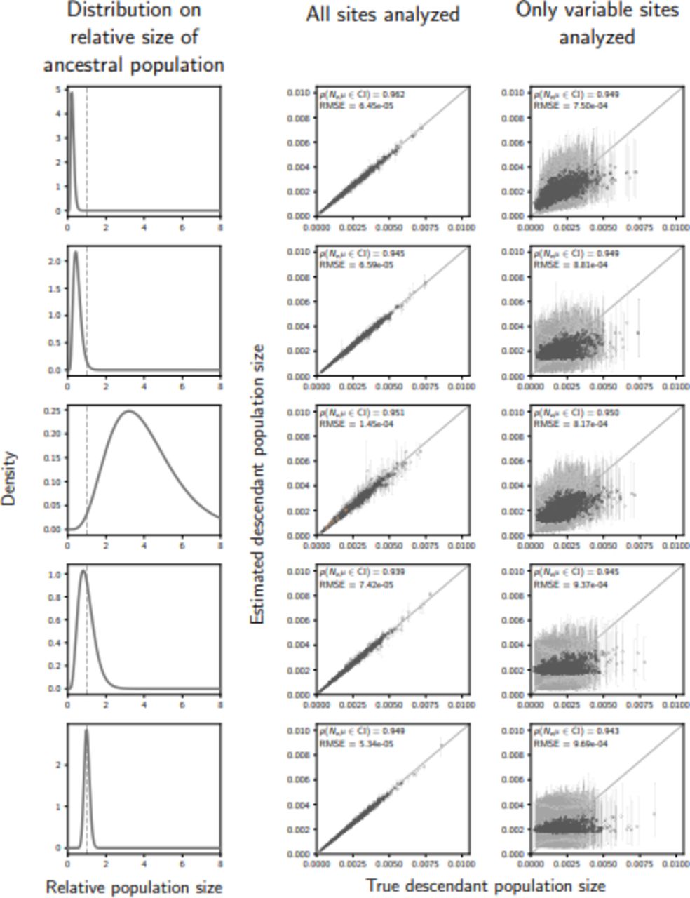
The accuracy and precision of demographic event time estimates (in units of expected subsitutions per site) when data are simulated and analyzed under the same model (i.e., no model misspecification), and event times are exponentially distributed with a mean of 0.01 (1.25 units of 4Ne generations). The left column of plots shows the gamma distribution from which the relative size of the ancestral population was drawn; this was also used as the prior when each simulated data set was analyzed. The center and right column of plots show true versus estimated values when using all characters (center) or only variable characters (right). Each plotted circle and associated error bars represent the posterior mean and 95% credible interval. Estimates for which the potential-scale reduction factor was greater than 1.2 (Brooks and Gelman, 1998) are highlighted in orange. Each plot consists of 1500 estimates—500 simulated data sets, each with three taxa. For each plot, the root-mean-square error (RMSE) and the proportion of estimates for which the 95% credible interval contained the true value—p(t ∈ CI)—is given. We generated the plot using matplotlib Version 2.0.0 (Hunter, 2007).

The performance of estimating the model of demographic changes when data are simulated and analyzed under the same model (i.e., no model misspecification), and event times are exponentially distributed with a mean of 0.01 (1.25 units of 4Ne generations). The left column of plots shows the gamma distribution from which the relative size of the ancestral population was drawn; this was also used as the prior when each simulated data set was analyzed. The center and right column of plots show true versus estimated values when using all characters (center) or only variable characters (right). Each plot shows the results of the analyses of 500 simulated data sets, each with three taxa; the number of data sets that fall within each possible cell of true versus estimated model is shown, and cells with more data sets are shaded darker. Each model is represented along the plot axes by three integers that indicate the divergence category of each pair of populations (e.g., 011 represents the model in which the second and third pair diverge at the same time, but separately from the first). The estimates are based on the model with the maximum a posteriori probability (MAP). For each plot, the proportion of data sets for which the model with the largest posterior probability matched the true model—  —is shown in the upper left corner, and the median posterior probability of the correct model across all data sets—
 —is shown in the upper right corner. We generated the plot using matplotlib Version 2.0.0 (Hunter, 2007).
A.1 Gamma(shape = 10, mean = 0.25) (4-fold population increase)
A.2 Gamma(shape = 10, mean = 0.5) (2-fold population increase)
A.3 Gamma(shape = 10, mean = 2) (2-fold population decrease)
A.4 Gamma(shape = 10, mean = 1) (no change on average, but a fair amount of variance)
A.5 Gamma(shape = 100, mean = 1) (no change on average, little variance)
The last distribution was chosen to represent a “worst-case” scenario where there was almost no demographic change in the history of the populations. For the mutation-scaled effective size of the descendant populations ( µ; i.e., the population size after the demographic change), we used a gamma distribution with a shape of 5 and mean of 0.002. The timing of the demographic events was exponentially distributed with a mean of 0.01 expected substitutions per site; given the mean of our distribution on the effective size of the descendant populations, this puts the expectation of demographic-change times in units of 4Ne generations at 1.25. This distribution on times was chosen to span times of demographic change from very recent (i.e., most gene lineages coalesce before the change) to old (i.e., most gene lineages coalesce after the change). The assignment of the three simulated populations to 1− −3 demographic events was controlled by a Dirichlet process with a mean number of 2.0 demographic events across the three populations. We generated 500 data sets under each of these five simulation conditions, all of which were analyzed using the same simulated distributions as priors.
Simulation conditions chosen to improve performance
Estimates of the timing and sharing of demographic events were quite poor across all the initial simulation conditions (see results). In an effort to find conditions under which the timing and sharing of demographic changes could be better estimated, and avoid combinations of parameter values that caused identifiability problems, we next explored simulations under distributions on times and population sizes offset from zero, but with much more recent demographic event times. For the mutation-scaled effective size of the descendant population  , we used an offset gamma distribution with a shape of 4, offset of 0.0001, and mean of 0.0021 (accounting for the offset). For the distribution of event times, we used a gamma distribution with a shape of 4, offset of 0.0001, and a mean of 0.002 (accounting for the offset; 0.25 units of 4Ne generations, on average). Again, we used five different distributions on the relative effective size of the ancestral population (see left column of Figures 4 and 5):

The accuracy and precision of demographic event time estimates (in units of expected subsitutions per site) when data are simulated and analyzed under the same model (i.e., no model misspecification), and event times are gamma-distributed with a shape of 4, offset of 0.0001, and mean of 0.002 (0.25 units of 4Ne generations). The left column of plots shows the gamma distribution from which the relative size of the ancestral population was drawn; this was also used as the prior when each simulated data set was analyzed. The center and right column of plots show true versus estimated values when using all characters (center) or only variable characters (right). Each plotted circle and associated error bars represent the posterior mean and 95% credible interval. Estimates for which the potential-scale reduction factor was greater than 1.2 (Brooks and Gelman, 1998) are highlighted in orange. Each plot consists of 1500 estimates—500 simulated data sets, each with three taxa. For each plot, the root-mean-square error (RMSE) and the proportion of estimates for which the 95% credible interval contained the true value—p(t ∈n CI)—is given. We generated the plot using matplotlib Version 2.0.0 (Hunter, 2007).

The performance of estimating the model of demographic changes when data are simulated and analyzed under the same model (i.e., no model misspecification), and event times are gamma-distributed with a shape of 4, offset of 0.0001, and mean of 0.002 (0.25 units of 4Ne generations). The left column of plots shows the gamma distribution from which the relative size of the ancestral population was drawn; this was also used as the prior when each simulated data set was analyzed. The center and right column of plots show true versus estimated values when using all characters (center) or only variable characters (right). Each plot shows the results of the analyses of 500 simulated data sets, each with three taxa; the number of data sets that fall within each possible cell of true versus estimated model is shown, and cells with more data sets are shaded darker. Each model is represented along the plot axes by three integers that indicate the divergence category of each pair of populations (e.g., 011 represents the model in which the second and third pair diverge at the same time, but separately from the first). The estimates are based on the model with the maximum a posteriori probability (MAP). For each plot, the proportion of data sets for which the model with the largest posterior probability matched the true model—  —is shown in the upper left corner, and the median posterior probability of the correct model across all data sets—
 —is shown in the upper right corner. We generated the plot using matplotlib Version 2.0.0 (Hunter, 2007).
B.1 Gamma(shape = 5, offset = 0.05, mean = 0.25) (4-fold population increase)
B.2 Gamma(shape = 5, offset = 0.05, mean = 0.5) (2-fold population increase)
B.3 Gamma(shape = 5, offset = 0.05, mean = 4) (4-fold population decrease)
B.4 Gamma(shape = 5, offset = 0.05, mean = 1) (no change on average, but a fair amount of variation)
B.5 Gamma(shape = 50, offset = 0, mean = 1) (no change on average, little variance)
We generated 500 data sets under each of these five distributions, all of which were analyzed under priors that matched the generating distributions.
2.3.2 Simulations to assess sensitivity to prior assumptions
Next, we simulated an additional 500 data sets under Condition B.1 above. We then analyzed each of these data sets under “diffuse” prior distributions:
τ ∼ Exponential(mean = 0.005)
- ∼ Exponential(mean = 2)
- ∼ Gamma(shape = 2, mean = 0.002)


These distributions were chosen to reflect realistic amounts of prior uncertainty about the timing of demographic changes and past and present effective population sizes when analyzing empirical data. For comparison, we also performed the same simulations and analyses under diffuse priors for three divergence comparisons For these divergence comparisons, we simulated 10 sampled genomes per population to match the same total number of samples per comparison (20) as the demographic simulations.
2.3.3 Simulating a mix of divergence and demographic comparisons
To explore how well our method can infer a mix of shared demographic changes and divergence times, we simulated 500 data sets comprised of 6 comparisons: 3 demographic comparisons and 3 divergence comparisons. 20 genomes (10 diploid individuals) were sampled from each comparison; for divergence comparisons, 10 genomes were sampled from each of the two populations. We used the same simulation conditions described above for B.2. All simulated data sets were analyzed under priors that matched the generating distributions.
2.3.4 Simulating linked sites
To assess the effect of linked sites on the inference of the timing and sharing of demographic changes, we simulated data sets comprising 5000 100-base-pair loci (500,000 total characters). The distributions on parameters were the same as the conditions described for B.1 above. These same distributions were used as priors when analyzing the simulated data sets.
2.4 Empirical application to stickleback data
2.4.1 Assembly of loci
We assembled the publicly available RADseq data collected by Hohenlohe et al. (2010) from five populations of threespine sticklebacks (Gasterosteus aculeatus) from south-central Alaska. After downloading the reads mapped to the stickleback genome by Hohenlohe et al. (2010) from Dryad (doi:10.5061/dryad.b6vh6), We assembled reference guided alignments of loci in Stacks v1.48 Catchen et al. (2013) with a minimum read depth of 3 identical reads per locus within each individual and the bounded single-nucleotide polymorphism (SNP) model with error bounds between 0.001 and 0.01. To maximize the number of loci and minimize paralogy, we assembled each population separately; because ecoevolity models each population separately (Figure 1), the characters do not need to be orthologous across populations, only within them.
2.4.2 Inferring shared demographic changes with ecoevolity
We used a value for the concentration parameter of the Dirichlet process that corresponds to a mean number of events of three (α = 2.22543). We used the following prior distributions on the timing of events and effective sizes of populations:
τ ∼ Exponential(mean = 0.001)
- ∼ Exponential(mean = 1)
- ∼ Gamma(shape = 2, mean = 0.002)


To assess the sensitivity of the results to these prior assumptions, we also analyzed the data under two additional priors on the concentration parameter, event times, and relative effective population size of the ancestral population:
α = 13 (half of prior probability on 5 events)
α = 0.3725 (half of prior probability on 1 event)
τ ∼ Exponential(mean = 0.0005)
τ ∼ Exponential(mean = 0.01)
- ∼ Exponential(mean = 0.5)
- ∼ Exponential(mean = 0.1)


For each prior setting, we ran 10 MCMC chains for 150,000 generations, sampling every 100 generations; we did this using all the sites in the assembled stickleback loci and only SNPs. To assess convergence and mixing of the chains, we calculated the potential scale reduction factor (PSRF; the square root of Equation 1.1 in Brooks and Gelman, 1998) and effective sample size (Gong and Flegal, 2016) of all continuous parameters and the log likelihood using the pyco-sumchains tool of pycoevolity (Version 0.1.2 Commit 89d90a1). We also visually inspected the sampled log likelihood and parameters values over generations with the program Tracer Version 1.6 (Rambaut et al., 2014). The MCMC chains for all analyses converged almost immediatley; we conservatively removed the first 101 samples from each chain, resulting in 14,000 samples from the posterior (1400 samples from 10 chains) for each analysis.
3 Results & Discussion
3.1 Analyses of simulated data
3.1.1 Estimating timing and sharing of demographic changes
Despite our attempt to capture a mix of favorable and challenging parameter values, estimates of the timing (Figure 2) and sharing (Figure 3) of demographic events were quite poor across all the simulation conditions we initially explored. Under the “worst-case” scenario of very little population-size change (bottom row of Figures 2 and 3), our method is unable to identify the timing or model of demographic change. As expected, our method returns the prior on the timing of events (bottom row of Figure 2) and almost always prefers either a model with a single, shared demographic event (model “000”) or independent demographic changes (model “012”; bottom row of Figure 3). This is expected behavior, because there is essentially no information in the data about the timing of demographic changes, and a Dirichlet process with a mean of 2.0 demographic events, puts approximately 0.24 of the prior probability on the models with one and three events, and 0.515 prior probability on the three models with two events (approximately 0.17 each). Thus, with little information, the method samples from the prior distribution on the timing of events, and prefers one of the two models with larger prior probability.
Under considerable changes in population size, the method only fared moderately better at estimating the timing of demographic events (top three rows of Figure 2). The ability to identify the model improved under these conditions, but the frequency at which the correct model was preferred only exceeded 50% for the large population expansions (top three rows of Figure 3). The median posterior support for the correct model was very small (less than 0.58) under all conditions. Under all simulation conditions, estimates of the timing and sharing of demographic events are better when using all characters, rather than only variable characters (second versus third column of Figures 2 and 3). Likewise, we see better estimates of effective population sizes when using the invariant characters (Figures S1 and S2).

The accuracy and precision of estimates of the effective size (scaled by the mutation rate) of the population before a demographic change (“ancestral” population) when data are simulated and analyzed underthe same model (i.e., no model misspecification), and event times are exponentially distributed with a mean of 0.01 (1.25 units of 4Ne generations). The left column of plots shows the gamma distribution from which the relative size of the ancestral population was drawn; this was also used as the prior when each simulated data set was analyzed. The center and right column of plots show true versus estimated values when using all characters (center) or only variable characters (right). Each plotted circle and associated error bars represent the posterior mean and 95% credible interval. Estimates for which the potential-scale reduction factor was greater than 1.2 (Brooks and Gelman, 1998) are highlighted in orange. Each plot consists of 1500 estimates—500 simulated data sets, each with three taxa. For each plot, the root-mean-square error (RMSE) and the proportion of estimates for which the 95% credible interval contained the true value—p(Neµ ∈ CI)—is given. We generated the plot using matplotlib Version 2.0.0 (Hunter, 2007)

The accuracy and precision of estimates of the effective size (scaled by the mutation rate) of the population after a demographic change (“descendant” population) when data are simulated and analyzed underthe same model (i.e., no model misspecification), and event times are exponentially distributed with a mean of 0.01 (1.25 units of 4Ne generations). The left column of plots shows the gamma distribution from which the relative size of the ancestral population was drawn; this was also used as the prior when each simulated data set was analyzed. The center and right column of plots show true versus estimated values when using all characters (center) or only variable characters (right). Each plotted circle and associated error bars represent the posterior mean and 95% credible interval. Estimates for which the potential-scale reduction factor was greater than 1.2 (Brooks and Gelman, 1998) are highlighted in orange. Each plot consists of 1500 estimates—500 simulated data sets, each with three taxa. For each plot, the root-mean-square error (RMSE) and the proportion of estimates for which the 95% credible interval contained the true value—p(Neµ ∈ CI)—is given. We generated the plot using matplotlib Version 2.0.0 (Hunter, 2007)
We observed numerical problems when the time of the demographic change was either very recent or old relative to the effective size of the population following the change ( ; the descendant population). In such cases, either very few or almost all of the sampled gene copies coalesce after the demographic change, providing almost no information about the magnitude or timing of the population-size change. In these cases, the data are well-explained by a constant population size, which can be achieved by the model in three ways: (1) an expansion time of zero and an ancestral population size that matched the true population size, (2) an old expansion and a descendant population size that matched the true population size, or (3) an intermediate expansion time and both the ancestral and descendant sizes matched the true size. The true population size being matched in these modelling conditions is that of the descendant or ancestral population if the expansion was old or recent, respectively. This caused MCMC chains to converge to different regions of parameter space (highlighted in orange in Figure 2).
Even after we tried selecting simulation conditions that are more favorable for identifying the event times, estimates of the timing and sharing of demographic events remain quite poor (Figures 4 and 5). Under the recent (but not too recent) 4-fold population-size increase (on average) scenario, we do see better estimates of the times of the demographic change (top row of Figure 4), but the ability to identify the correct number of events and the assignment of the populations to those events remains quite poor; the correct model is preferred only 57% of the time, and the median posterior probability of the correct model is only 0.42 (top row of Figure 5). Under the most extreme population retraction scenario (4-fold, on average), the correct model is preferred only 40% of the time, and the median posterior probability of the correct model is only 0.26 (middle row of Figure 5). Estimates are especially poor when using only variable characters, so we focus on the results using all characters (second versus third column of Figures 2 and 3); we also see worse estimates of population sizes when excluding invariant characters (Figures S3 and S4).

The accuracy and precision of estimates of the effective size (scaled by the mutation rate) of the population before a demographic change (“ancestral” population) when data are simulated and analyzed underthe same model (i.e., no model misspecification), and event times are gamma-distributed with a shape of 4, offset of 0.0001, and mean of 0.002 (0.25 units of 4Ne generations). The left column of plots shows the gamma distribution from which the relative size of the ancestral population was drawn; this was also used as the prior when each simulated data set was analyzed. The center and right column of plots show true versus estimated values when using all characters (center) or only variable characters (right). Each plotted circle and associated error bars represent the posterior mean and 95% credible interval. Estimates for which the potential-scale reduction factor was greater than 1.2 (Brooks and Gelman, 1998) are highlighted in orange. Each plot consists of 1500 estimates—500 simulated data sets, each with three taxa. For each plot, the root-mean-square error (RMSE) and the proportion of estimates for which the 95% credible interval contained the true value—p(Neµ ∈ CI)—is given. We generated the plot using matplotlib Version 2.0.0 (Hunter, 2007)

The accuracy and precision of estimates of the effective size (scaled by the mutation rate) of the population after a demographic change (“descendant” population) when data are simulated and analyzed underthe same model (i.e., no model misspecification), and event times are gamma-distributed with a shape of 4, offset of 0.0001, and mean of 0.002 (0.25 units of 4Ne generations). The left column of plots shows the gamma distribution from which the relative size of the ancestral population was drawn; this was also used as the prior when each simulated data set was analyzed. The center and right column of plots show true versus estimated values when using all characters (center) or only variable characters (right). Each plotted circle and associated error bars represent the posterior mean and 95% credible interval. Estimates for which the potential-scale reduction factor was greater than 1.2 (Brooks and Gelman, 1998) are highlighted in orange. Each plot consists of 1500 estimates—500 simulated data sets, each with three taxa. For each plot, the root-mean-square error (RMSE) and the proportion of estimates for which the 95% credible interval contained the true value—p(Neµ ∈ CI)—is given. We generated the plot using matplotlib Version 2.0.0 (Hunter, 2007).
3.1.2 Sensitivity to prior assumptions
Above, we observe the best estimates of the timing and sharing of demographic events under narrow distributions on the relative effective size of the ancestral population (top row of Figures 2–5), which were used to both simulate the data and as the prior when those data were analyzed. These distributions are unrealistically informative priors for empirical studies, for which there is usually little a priori information about past population sizes. Our results show that the better performance under these distributions was at least partially caused by greater prior information, and that inference of shared demographic events is much more sensitive to prior assumptions than shared divergences (Figures 6 and 7).

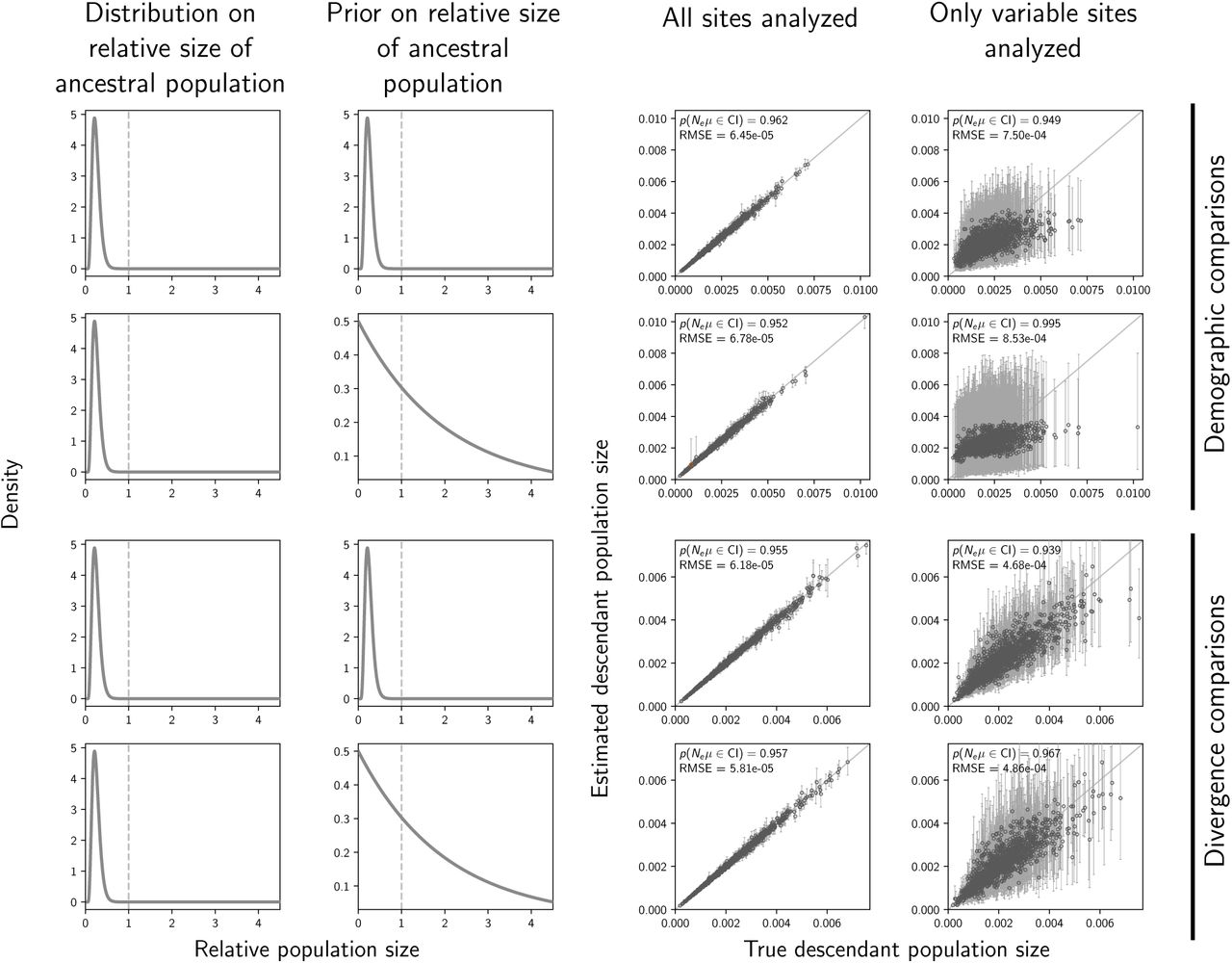
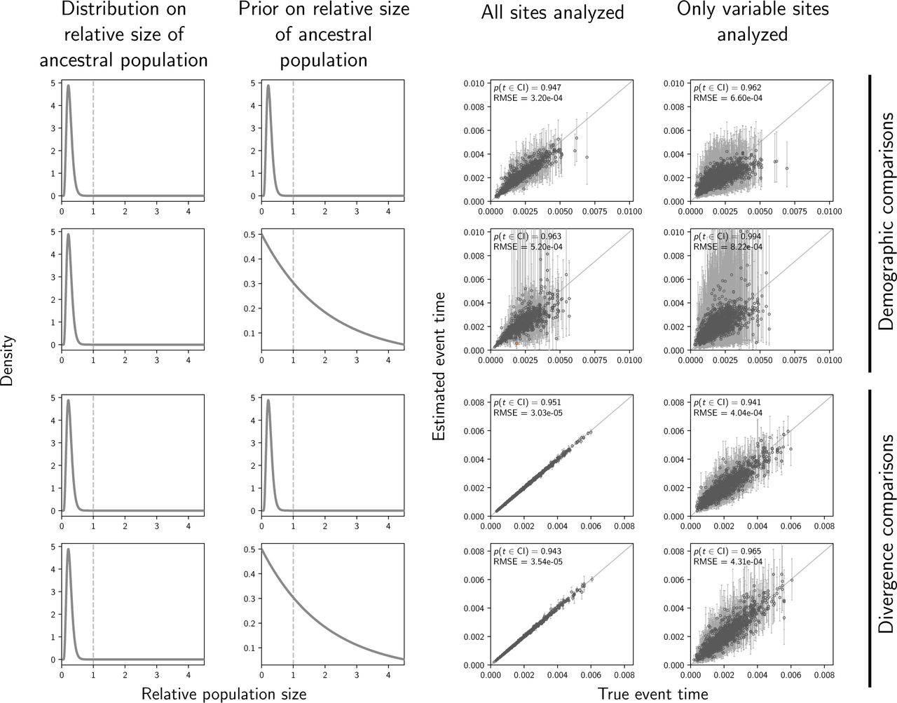
The accuracy and precision of time estimates of demographic changes (top two rows) versus divergences (bottom two rows) when the priors are correct (first and third rows) versus when the priors are diffuse (second and fourth rows). Time is measured in units of expected subsitutions per site. The first and second columns of plots show the distribution on the relative effective size of the ancestral population for simulating the data (first column) and for the prior when analyzing the simulated data (second column). The third and fourth columns of plots show true versus estimated values when using all characters (center) or only variable characters (right). Each plotted circle and associated error bars represent the posterior mean and 95% credible interval. Estimates for which the potential-scale reduction factor was greater than 1.2 (Brooks and Gelman, 1998) are highlighted in orange. Each plot consists of 1500 estimates—500 simulated data sets, each with three taxa. For each plot, the root-mean-square error (RMSE) and the proportion of estimates for which the 95% credible interval contained the true value— p(t ∈ CI)—is given. The first row of plots are repeated from Figure 4 for comparison. We generated the plot using matplotlib Version 2.0.0 (Hunter, 2007).

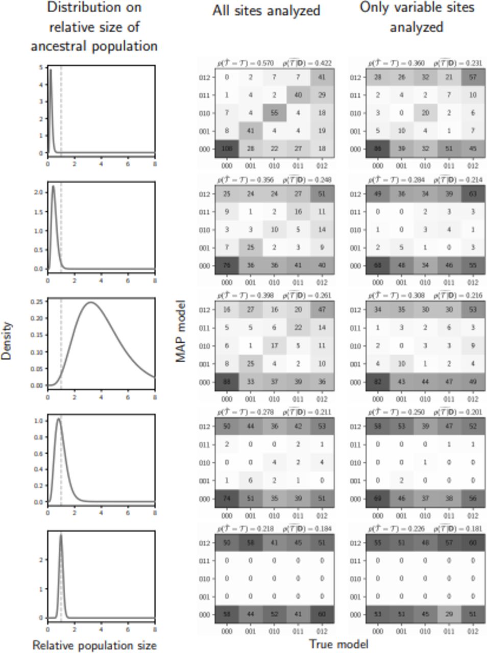
The performance of estimating the model of demographic changes (top two rows) versus model of divergences (bottom two rows) when the priors are correct (first and third rows) versus when the priors are diffuse (second and fourth rows). The first and second columns of plots show the distribution on the relative effective size of the ancestral population for simulating the data (first column) and for the prior when analyzing the simulated data (second column). The third and fourth columns of plots show true versus estimated values when using all characters (center) or only variable characters (right). Each plot shows the results of the analyses of 500 simulated data sets, each with three taxa; the number of data sets that fall within each possible cell of true versus estimated model is shown, and cells with more data sets are shaded darker. Each model is represented along the plot axes by three integers that indicate the divergence category of each pair of populations (e.g., 011 represents the model in which the second and third pair diverge at the same time, but separately from the first). The estimates are based on the model with the maximum a posteriori probability (MAP). For each plot, the proportion of data sets for which the model with the largest posterior probability matched the true model— —is shown in the upper left corner, and the median posterior probability of the correct model across all data sets—
 —is shown in the upper right corner. The first row of plots are repeated from Figure 5 for comparison. We generated the plot using matplotlib Version 2.0.0 (Hunter, 2007).
The precision of time estimates of demographic changes decreases substantially under the diffuse priors (top two rows of Figure 6), whereas the precision of the divergence-time estimates is high and largely unchanged under the diffuse priors (bottom two rows of Figure 6). We see the same patterns in the estimates of population sizes (Figures S5 and S6)

The accuracy and precision of estimates of the effective size (scaled by the mutation rate) of the ancestral population of demographic comparisons (top two rows) versus divergence comparisons (bottom two rows) when the priors are correct (first and third rows) versus when the priors are diffuse (second and fourth rows). The first and second columns of plots show the distribution on the relative effective size of the ancestral population for simulating the data (first column) and for the prior when analyzing the simulated data (second column). The third and fourth columns of plots show true versus estimated values when using all characters (center) or only variable characters (right). Each plotted circle and associated error bars represent the posterior mean and 95% credible interval. Estimates for which the potential-scale reduction factor was greater than 1.2 (Brooks and Gelman, 1998) are highlighted in orange. Each plot comprises 500 simulated data sets, each with three taxa. For each plot, the root-mean-square error (RMSE) and the proportion of estimates for which the 95% credible interval contained the true value—p(Neµ ∈ CI)—is given. The first row of plots are repeated from Figure S3 for comparison. We generated the plot using matplotlib Version 2.0.0 (Hunter, 2007).
The accuracy and precision of estimates of the effective size (scaled by the mutation rate) of the descendant population(s) of demographic comparisons (top two rows) versus divergence comparisons (bottom two rows) when the priors are correct (first and third rows) versus when the priors are diffuse (second and fourth rows). The first and second columns of plots show the distribution on the relative effective size of the ancestral population for simulating the data (first column) and for the prior when analyzing the simulated data (second column). The third and fourth columns of plots show true versus estimated values when using all characters (center) or only variable characters (right). Each plotted circle and associated error bars represent the posterior mean and 95% credible interval. Estimates for which the potential-scale reduction factor was greater than 1.2 (Brooks and Gelman, 1998) are highlighted in orange. Each plot comprises 500 simulated data sets, each with three taxa. For each plot, the root-mean-square error (RMSE) and the proportion of estimates for which the 95% credible interval contained the true value—p(Neµ ∈ CI)—is given. The first row of plots are repeated from Figure S4 for comparison. We generated the plot using matplotlib Version 2.0.0 (Hunter, 2007).
Under more realistic, diffuse priors, the probability of inferring the correct model of demographic events decreases from 0.57 to 0.434 when all characters are used, and from 0.36 to 0.284 when only variable characters are used (top two rows of Figure 7). The median posterior probability of the correct model also decreases from 0.422 to 0.292 when all characters are used, and from 0.231 to 0.178 when only variable characters are used (top two rows of Figure 7). Most importantly, we see a strong bias toward underestimating the number of events under the more realistic diffuse priors (top two rows of Figure 7). In comparison, the inference of shared divergences is much more accurate and precise than shared demographic changes, and is much more robust to the diffuse priors (bottom two rows of Figure 7). When all characters are used, under both the correct and diffuse priors, the correct divergence model is preferred over 91% of the time, and the median posterior probability of the correct model is over 0.93.
3.2 Inferring a mix of shared divergences and demographic changes
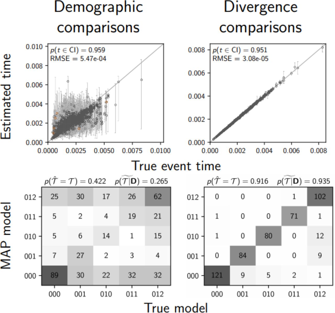
When demographic and divergence comparisons are analyzed separately, the performance of estimating the timing and sharing of demographic changes and divergences is dramatically different, with the latter being much more accurate and precise than the former (e.g., see Figures 7 and 6). One might hope that if we analyze a mix of demographic and divergence comparisons, the informativeness of the divergence times can help “anchor” and improve the estimates of shared demographic changes. However, our results from simulating data sets comprising a mix of three demographic and three divergence comparisons rule out this possibility.
When analyzing a mix of demographic and divergence comparisons, the ability to infer the timing and sharing of demographic changes remains poor, whereas estimates of shared divergences remain accurate and precise (Figure 8). The estimates of the timing and sharing of demographic events are very similar to when we simulated and analyzed only three demographic comparisons under the same distributions on event times and population sizes (compare left column of Figure 8 to the second row of Figures 4 and 5). The same is true for the estimates of population sizes (Figure S7). Thus, there does not appear to be any mechanism by which the more informative divergence-time estimates “rescue” the estimates of the timing and sharing of the demographic changes.

Analyses of six taxa comprising a mix of three populations that experienced a demogrpahic change and three pairs of populations that diverged. The performance of estimating the timing of events (Row 1), sharing of events (Rows 2–3), ancestral population size (Row 4), and descendant population size (Row 5) are shown separately for the three populations that experienced a demographic change (Columns 1 and 2) and the three pairs of populations that diverged (Columns 3 and 4). The plots of the demographic comparisons (Columns 1 and 2) are comparable to the second column of Figures 4, 5, S4, and S3; the same priors on event times and ancestral population size were used. Estimates for which the potential-scale reduction factor was greater than 1.2 (Brooks and Gelman, 1998) are highlighted in orange. Each plot shows the results from 500 simulated data sets, each with six taxa. We generated the plot using matplotlib Version 2.0.0 (Hunter, 2007).

Analyses of six taxa comprising a mix of three populations that experienced a demogrpahic change and three pairs of populations that diverged. The performance of estimating the timing (top row) and sharing (bottom row) of events are shown separately for the three populations that experienced a demographic change (left column) and the three pairs of populations that diverged (right column). The plots of the demographic comparisons (left column) are comparable to the second column of Figures 4 and 5; the same priors on event times and ancestral population size were used. Time estimates for which the potential-scale reduction factor was greater than 1.2 (Brooks and Gelman, 1998) are highlighted in orange. Each plot shows the results from 500 simulated data sets, each with six taxa. We generated the plot using matplotlib Version 2.0.0 (Hunter, 2007).
3.3 The effect of linked sites
Most reduced-representation genomic datasets are comprised of loci of contiguous, linked nucleotides. Thus, when using the method presented here that assumes each character is effectively unlinked (i.e., evolved along a gene tree that is independent from other characters, conditional on the population history), one either has to violate this assumption, or discard all but (at most) one site per locus. Given that all the results above indicate better estimates when all characters are used (compared to using only variable characters), we simulated linked sites to determine which strategy is better: analyzing all linked sites and violating the assumption of unlinked characters, or discarding all but (at most) one variable character per locus.
The results are almost identical to when all the sites were unlinked (compare first row of Figures 4 and 5 to Figure 9, and the first row of Figures S3 and S4 to the bottom two rows of Figure S8). Thus, violating the assumption of unlinked sites has little affect on the estimation of the timing and sharing of demographic changes; this is also true for estimates of population sizes (Figure S8). This is consistent with the findings of Oaks (2019) and Oaks et al. (2019) that the violation of linked sites had little affect on the estimation of shared divergence times. These results suggest that analyzing all of the sites in loci assembled from reduced-representation genomic libraries (e.g., sequence-capture or RADseq loci) is a better strategy than excluding sites to avoid violating the assumption of unlinked characters.

Results of analyses of simulated data sets with 5000 100-base-pair loci when using all characters (left column) or only unlinked variable characters (right column). The plots are comparable to the first row of Figures 4, 5, S4, and S3; the models were identical, the only difference is the linkage of characters into loci. Estimates for which the potential-scale reduction factor was greater than 1.2 (Brooks and Gelman, 1998) are highlighted in orange. Each plot shows the results from 500 simulated data sets, each with six taxa. We generated the plot using matplotlib Version 2.0.0 (Hunter, 2007).

Results of analyses of simulated data sets with 5000 100-base-pair loci when using all characters (left column) or only unlinked variable characters (right column). The plots are comparable to the first row of Figures 4 and 5; the models were identical, the only difference is the linkage of characters into loci. Time estimates for which the potential-scale reduction factor was greater than 1.2 (Brooks and Gelman, 1998) are highlighted in orange. Each plot shows the results from 500 simulated data sets, each with six taxa. We generated the plot using matplotlib Version 2.0.0 (Hunter, 2007).
3.4 Reassessing the co-expansion of stickleback populations
Using an ABC analog to the model of shared demographic changes developed here, Xue and Hickerson (2015) found very strong support (0.99 posterior probability) that five populations of threespine sticklebacks (Gasterosteus aculeatus) from south central Alaska recently co-expanded. This inference was based on the publicly available RADseq data collected by Hohenlohe et al. (2010) (https://trace.ncbi.nlm.nih.gov/Traces/sra/?study=SRP001747; NCBI Short Read Archive accession numbers SRX015871–SRX015877). We re-assembled and analyzed these data under our full-likelihood Bayesian framework, both using all sites from assembled loci and only SNPs.
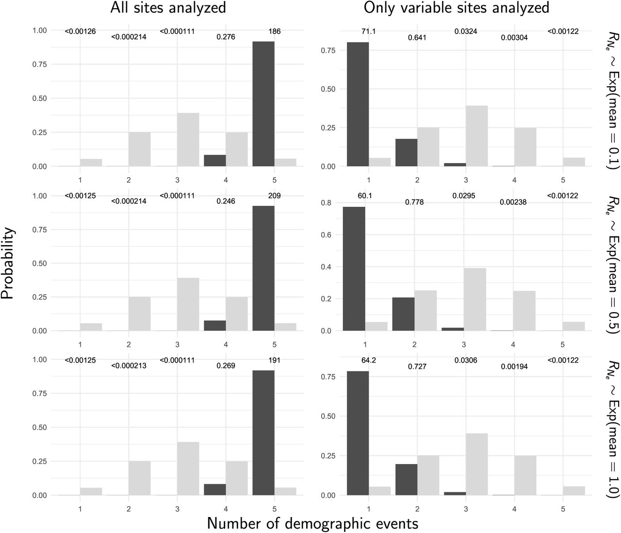
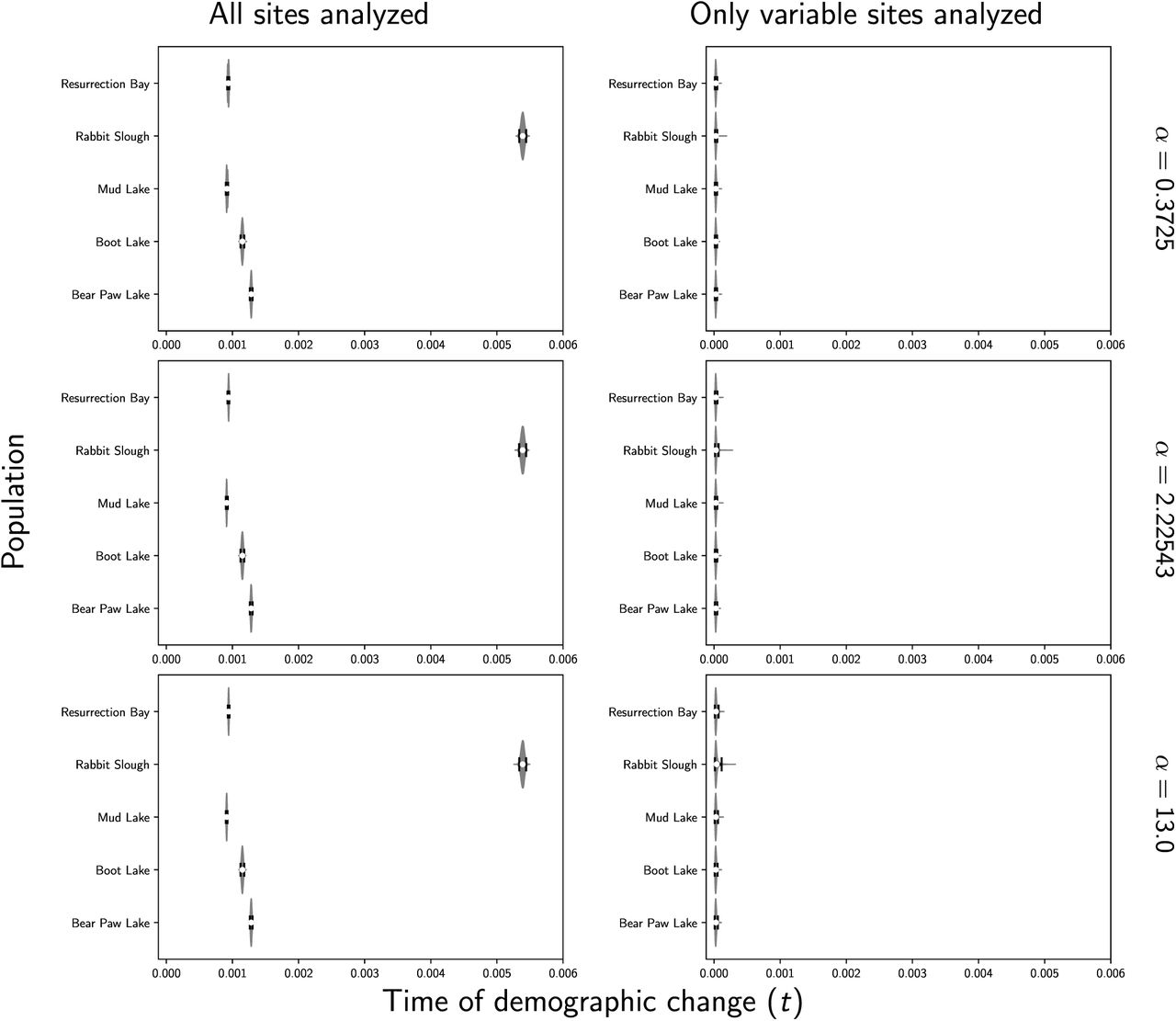
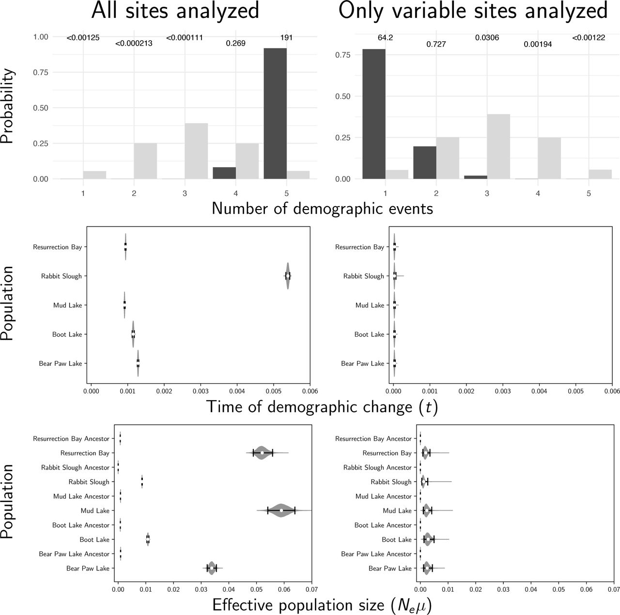
Stacks produced a concatenated alignment of all loci with 2,115,588, 2,166,215, 2,081,863, 2,059,650, and 2,237,438 total sites and 118,462, 89,968, 97,557, 139,058, and 103,271 variable sites for the Bear, Boot, Mud, Rabbit, and Resurrection stickleback populations respectively. When analyzing all sites from the assembled stickleback RADseq data, we find strong support for five independent population expansions (no shared demographic events; Figure 10). In sharp contrast, when analyzing only SNPs, we find support for a single, shared, extremely recent population expansion (Figure 10). The support for a single, shared event is consistent with the results from our simulations using diffuse priors and only including SNPs, which showed consistent, spurious support for a single event (Row 2 of Figure 7). These results are relatively robust to a broad range of prior assumptions (Figures S9–17).

The prior (light bars) and posterior (dark bars) probabilities of the number of demographic events across five stickleback populations when all of the sites (left column) or only variable sites (right column) of the RADseq alignments are analyzed. Each row shows results under a different prior on the concentration parameter of the dirichlet process. We generated the plots with ggplot2 Version 2.2.1 (Wickham, 2009).

Estimates of the time of a change in population size across five stickleback populations when all of the sites (left column) or only variable sites (right column) of the RADseq alignments are analyzed. Each row shows results under a different prior on the concentration parameter of the dirichlet process. We generated the plot using matplotlib Version 2.0.0 (Hunter, 2007).

Estimates of the effective population size before (“ancestor”) and after a demographic change across five stickleback populations when all of the sites (left column) or only variable sites (right column) of the RADseq alignments are analyzed. Each row shows results under a different prior on the concentration parameter of the dirichlet process. We generated the plot using matplotlib Version 2.0.0 (Hunter, 2007).

The prior (light bars) and posterior (dark bars) probabilities of the number of demographic events across five stickleback populations when all of the sites (left column) or only variable sites (right column) of the RADseq alignments are analyzed. Each row shows results under a different prior on the timing of the change in population size. We generated the plots with ggplot2 Version 2.2.1 (Wickham, 2009).

Estimates of the time of a change in population size across five stickleback populations when all of the sites (left column) or only variable sites (right column) of the RADseq alignments are analyzed. Each row shows results under a different prior on the timing of the change in population size. We generated the plot using matplotlib Version 2.0.0 (Hunter, 2007).

Estimates of the effective population size before (“ancestor”) and after a demographic change across five stickleback populations when all of the sites (left column) or only variable sites (right column) of the RADseq alignments are analyzed. Each row shows results under a different prior on the timing of the change in population size. We generated the plot using matplotlib Version 2.0.0 (Hunter, 2007).
The prior (light bars) and posterior (dark bars) probabilities of the number of demographic events across five stickleback populations when all of the sites (left column) or only variable sites (right column) of the RADseq alignments are analyzed. Each row shows results under a different prior on the relative effective size of the ancestral population. We generated the plots with ggplot2 Version 2.2.1 (Wickham, 2009).

Estimates of the time of a change in population size across five stickleback populations when all of the sites (left column) or only variable sites (right column) of the RADseq alignments are analyzed. Each row shows results under a different prior on the relative effective size of the ancestral population. We generated the plot using matplotlib Version 2.0.0 (Hunter, 2007).

Estimates of the effective population size before (“ancestor”) and after a demographic change across five stickleback populations when all of the sites (left column) or only variable sites (right column) of the RADseq alignments are analyzed. Each row shows results under a different prior on the relative effective size of the ancestral population. We generated the plot using matplotlib Version 2.0.0 (Hunter, 2007).

Estimates of the number (Row 1), timing (Row 2), and magnitude (Row 3) of demographic events across five stickleback populations, when using all sites (left column) or only variable sites (right column). We used an exponentially distributed prior with a mean of 0.001 on event times, an exponentially distributed prior with a mean of 1 on the relative ancestral effective population size, and a gamma-distributed prior (shape = 2, mean = 0.002) on the descendant population sizes. For the number of events (Row 1), the light and dark bars represent the prior and posterior probabilities, respectively. Time (Row 2) is in units of expected subsitutions per site. For the violin plots, each plotted circle and associated error bars represent the posterior mean and 95% credible interval. Bar graphs were generated with ggplot2 Version 2.2.1 (Wickham, 2009); violin plots were generated with matplotlib Version 2.0.0 (Hunter, 2007).
When using only SNPs, estimates of the timing of the single, shared demographic event are essentially at the minimum of zero, suggesting that there is little information about the timing of any demographic changes in the SNP data alone. This is consistent with results of Xue and Hickerson (2015) where the single, shared event was also estimated to have occurred at the minimum (1000 generations) of their uniform prior on the timing of demographic changes. Their and our results based solely on SNPs seem to be an artifact of the lack of information in the SNP-only data. Based on our simulation results, our estimates using all of the sites in the stickleback RADseq loci should be the most accurate. However, the unifying theme of our simulation results is that all estimates of shared demographic events tend to be poor and should be treated with a lot of skepticism.
4 Conclusions
There is a narrow temporal window within which we can reasonably estimate the time of a demographic change. The width of this window is determined by how deep in the past the change occurred relative to the effective size of the population (i.e., in coalescent units). If too old or recent, there are too few coalescence events before or after the demographic change, respectively, to provide information about the effective size of the population. When we are careful to simulate data within this window, and the change in population size is large enough, we can estimate the time of the demographic changes reasonably well (e.g., see the top row of Figure 4). However, even under these condtions, the ability to correctly infer the number of demographic events, and the assignment of populations to those events is quite limited (Figure 5). When only variable characters are analyzed (i.e., SNPs), estimates of the timing and sharing of demographic changes are consistently bad; we see this across all the conditions we simulated. Most alarmingly, when the priors are more diffuse than the distributions that generated the data, as will be true in most empirical applications, there is a strong bias toward estimating too few demographic events (i.e., over-clustering comparisons to demographic events; Row 2 of Figure 7), especially when only variable characters are analyzed. These results help explain the stark contrast we see in our results from the stickleback RADseq data when including versus excluding constant sites (Figure 10). These findings are in sharp contrast to estimating shared divergence times, which is much more accurate, precise, and robust to prior assumptions (Figures 6–8 Oaks, 2019; Oaks et al., 2019).
Given the poor estimates of co-demographic changes, even when all the information in the data are leveraged by a full-likelihood method, any inference of shared demographic changes should be treated with caution. However, there are potential ways that estimates of shared demographic events could be improved. For example, modelling loci of contiguous, linked sites could help extract more information about past demographic changes. Longer loci can contain much more information about the lengths of branches in the gene tree, which are critically informative about the size of the population through time. This is evidenced by the extensive literature on powerful “skyline plot” and “phylodynamic” methods (Pybus et al., 2000; Strimmer and Pybus, 2001; Opgen-Rhein et al., 2005; Drummond et al., 2005; Heled and Drummond, 2008; Minin et al., 2008; Ho and Shapiro, 2011; Palacios and Minin, 2013, 2012; Stadler et al., 2013; Gill et al., 2013; Palacios et al., 2014; Lan et al., 2015; Karcher et al., 2016, 2017; Faulkner et al., 2018; Karcher et al., 2019). With loci from across the genome, each with more information about the gene tree they evolved along, perhaps more information can be captured about temporally clustered changes in the rate of coalescence across populations. Another potential source of information could be captured by modelling recombination along large regions of chromosomes. By approximating the full coalescent process, many methods have been developed to model recombination in a computationally feasible manner (McVean and Cardin, 2005; Marjoram and Wall, 2006; Chen et al., 2009; Li and Durbin, 2011; Sheehan et al., 2013; Schiffels and Durbin, 2014; Rasmussen et al., 2014; Palacios et al., 2015). This could potentially leverage additional information from genomic data about the linkage patterns among sites along chromosomes. Both of the these avenues are worth pursuing given the myriad historical processes that predict patterns of temporally clustered changes in population sizes across populations.
5 Acknowledgments
We thank the members of the Phyletica Lab (the phyleticians) for helpful feedback on multiple drafts of this paper. This work was supported by funding provided to JRO from the National Science Foundation (NSF grant number DEB 1656004). NL was supported for a summer REU from NSF grant DEB 1656004 to JRO; NL also benefitted from an NSF REU award to Dr. Leslie Goertzen (grant number DBI 1560115). The computational work was made possible by the Auburn University (AU) Hopper Cluster supported by the AU Office of Information Technology and a grant of high-performance computing resources and technical support from the Alabama Supercomputer Authority. This paper is contribution number 899 of the Auburn University Museum of Natural History.
Appendix A The full model
A.1 The data
As described by Oaks (2019), we assume we have orthologous, biallelic genetic characters collected from taxa we wish to compare. By biallelic, we mean that each character has at most two states, which we refer to as “red” and “green” following Bryant et al. (2012). For each taxon, we either have these data from one or more individuals from a single population, in which case we infer the timing and extent of a population size change, or one or more individuals from two populations or species, in which case we infer the time when they diverged (Figure 1).
For each population and for each character we genotype n copies of the locus, r of which are copies of the red allele and the remaining n − r are copies of the green allele. Thus, for each population of a pair, and for each locus, we have a count of the total sampled gene copies and how many of those are the red allele.
Following the notation of Oaks (2019) we will use n and r to denote allele counts for a locus from either one population if we are modeling population-size change or both populations of a pair if we are modeling a divergence; i.e., n, r = (n, r) or n, r = (n1, r1), (n2, r2) (Figure 1 and Table 1). For convenience will use Di to denote these allele counts across all the loci from taxon i, which can be a single population or a pair of populations. Finally, we use D to represent the data across all the taxa for which we wish to compare times of either divergence or population-size change. Note, because the population of each compared taxon is modeled separately (Figure 1), characters do not have to be orthologous across taxa, only within them.
A key to some of the notation used in the text.
A.1.1 The evolution of markers
We assume each character evolved along a gene tree (g) according to a finite-sites, continuous-time Markov chain (CTMC) model. We assume the gene tree of each character is independent of the others, conditional on the population history (i.e., the characters are effectively unlinked). As the marker evolves along the gene tree, forward in time, there is a relative rate u of mutating from the red state to the green state, and a corresponding relative rate v of mutation from green to red (Bryant et al., 2012; Oaks, 2019). The stationary frequency of the green state is then π = u/(u + v). We will use µ to denote the overall rate of mutation. Evolutionary change is the product of µ and time. Thus, if µ = 1, time is measured in units of expected substitutions per site. Alternatively, if a mutation rate per site per unit time is given, then time is absolute.
A.1.2 The evolution of gene trees
We assume that the gene tree of each locus evolved within a simple “species” tree with one ancestral root population, which either left one or two descendant branches with different effective population sizes at time t (Figure 1). We will use ℕe to denote all the effective population sizes of a species tree;  and
and  when modeling a population-size change, and
  and
and  when modeling a divergence. Following Oaks (2019), we use S as shorthand for the species tree, which comprises the population sizes and divergence time of a pair (ℕe and t).
A.1.3 The likelihood
As in Oaks (2019), we use the work of Bryant et al. (2012) to analytically integrate over all possible gene trees and character substitution histories to compute the likelihood of the species tree directly from a biallelic character pattern under a coalescent model; p(n, r |S, µ, π). The only difference that is necessary is for population-size-change models that have a species tree with only one descendant population. Equation 19 of Bryant et al. (2012) shows how to obtain the partial likelihoods at the bottom of an ancestral branch from the partial likelihoods at the top of its two descendant branches. When there is only one descendant branch, this is simplified, and the partial likelihoods at the bottom of the ancestral branch are equal to the partial likelihoods at the top of its sole descendant branch. Other than this small change, the probability of a biallelic character pattern given the species tree, mutation rate, and equilibrium state frequencies (p(n, r | S, µ, π)) is calculated the same as in Bryant et al. (2012) and Oaks (2019).
For a given taxon, we can calculate the probability of all m loci from which we have data given the species tree and other parameters by assuming independence among loci (conditional on the species tree) and taking the product over them,
 We assume we biallelic data from 𝒩 taxa, which can be an arbitrary mix of (1) two populations or species for which t represents the time they diverged, or (2) one population for which t represents the time of a change in population size. The likelihood across all 𝒩 taxa is simply the product of the likelihood of each taxon,
 where D = D1, D2, …, D𝒩, S = S1, S2, …, S𝒩, µ = µ1, µ2, …, µ𝒩, and π = π1, π2, …, π𝒩. As described in Oaks (2019), if constant characters are not sampled for a taxon, we condition the likelihood for that taxon on only having sampled variable characters.
A.2 Bayesian inference
As described by Oaks (2019), we treat the number of events (population-size changes and/or divergences) and the assignment of taxa to those events as random variables under a Dirichlet process (Ferguson, 1973; Antoniak, 1974). We use 𝒯 to represent the partitioning of taxa to events, which we will also refer to as the “event model.” The concentration parameter, α, controls how clustered the Dirichlet process is, and determines the probability of all possible 𝒯 (i.e., all possible set partitions of taxa to 1, 2, …,𝒩 events). We use τ to represent the times of the unique events in 𝒯 Using this notation, the posterior distribution of our Dirichlet-process model is
 where Ne is the collection of the effective population sizes (ℕe) across all of the pairs.
A.2.1 Priors
Prior on the concentration parameter
Our implementation allows for a hierarchical approach to accommodeate uncertainty in the concentration parameter of the Dirichlet process by specifying a gamma distribution as a hyperprior on α (Escobar and West, 1995; Heath et al., 2011). Alternatively, α can also be fixed to a particular value, which is likely sufficient when the number of pairs is small.
Prior on the divergence times
Given the partitioning of taxa to events, we use a gamma distribution for the prior on the time of each event, τ|𝒯 ∼ Gamma(·, ·).
Prior on the effective population sizes
We use a gamma distribution as the prior on the the effective size of each descendant population of each taxon. Following Oaks (2019), we use a gamma distribution on the effective size of the ancestral population relative to the size of the descendant population(s), which we denote as  For a taxon with two descendant population (i.e., a divergence comparison), the ancestral population size is relative to the mean of the descendant populations. For a taxon with only one descendant population (i.e., a demographic comparison), the ancestral populations is relative to the size of that descendant.
Prior on mutation rates
We follow the same approach explained by Oaks (2019) to model mutation rates across taxa. The decision about how to model mutation rates is extremely important for any comparative phylogeographic approach that models taxa as disconnected species trees (Figure 1; e.g., Hickerson et al., 2006, 2007; Huang et al., 2011; Chan et al., 2014; Oaks, 2014; Xue and Hickerson, 2015; Burbrink et al., 2016; Xue and Hickerson, 2017; Gehara et al., 2017; Oaks, 2019). Time (τ) and mutation rate (µ) are inextricably linked, and because the comparisons are modeled as disconnected species trees, the data cannot inform the model about relative or absolute differences in µ among the comparisons. We provide flexibility to the investigator to fix or place prior probability distributions on the relative or absolute rate of mutation for each comparison. However, if one chooses to accommodate uncertainty in the mutation rate of one or more comparisons, the priors should be strongly informative. Because of the inextricable link between rate and time, placing a weakly informative prior on a comparison’s mutation rate prevents estimation of the time of its demographic change or divergence, which is the primary goal.
Prior on the equilibrium-state frequency
Recoding four-state nucleotides to two states requires some arbitrary decisions, and whenever π ≠ 0.5, these decisions can affect the likelihood of the model (Oaks, 2019). Because DNA is the dominant character type for genomic data, we assume that π = 0.5 in this paper. This makes the CTMC model of character-state substitution a two-state analog of the “JC69” model (Jukes and Cantor, 1969). However, if the genetic markers collected for one or more taxa are naturally biallelic, the frequencies of the two states can be meaningfully estimated, and our implementation allows for a beta prior on π in such cases. This makes the CTMC model of character-state substitution a two-state general time-reversible model (Tavaré, 1986).
A.2.2 Approximating the posterior with MCMC
We use Markov chain Monte Carlo (MCMC) algorithms to sample from the joint posterior in Equation 3. To sample across event models (𝒯) during the MCMC chain, we use the Gibbs sampling algorithm (Algorithm 8) of Neal (2000). We also use univariate and multivariate Metropolis-Hastings algorithms (Metropolis et al., 1953; Hastings, 1970) to update the model, the latter of which are detailed in Oaks (2019).
References


