

Abstract
A wide variety of human and non-human behavior is computationally well accounted for by probabilistic generative models, formalized consistently in a Bayesian framework. Recently, it has been suggested that another family of adaptive systems, namely, those governed by Darwinian evolutionary dynamics, are capable of implementing building blocks of Bayesian computations. These algorithmic similarities rely on the analogous competition dynamics of generative models and of Darwinian replicators to fit possibly high-dimensional and stochastic environments. Identified computational building blocks include Bayesian update over a single variable and replicator dynamics, transition between hidden states and mutation, and Bayesian inference in hierarchical models and multilevel selection. Here we provide a coherent mathematical discussion of these observations in terms of Bayesian graphical models and a step-by-step introduction to their evolutionary interpretation. We also extend existing results by adding two missing components: a correspondence between likelihood optimization and phenotypic adaptation, and between expectation-maximization-like dynamics in mixture models and ecological competition. These correspondences suggest a deeper algorithmic analogy between evolutionary dynamics and statistical learning, pointing towards a unified computational understanding of mechanisms Nature invented to adapt to high-dimensional and uncertain environments.
1 Introduction
The Bayesian framework of performing consistent computations about probabilistic beliefs has become a fundamental language to describe and understand adaptation in the presence of uncertainty [1, 2, 3]. Two factors have recently driven the theoretical development of this machinery: i) the machine learning revolution building on the boom of available data and computational power [4, 5] and ii) the possibility to perform large-scale (human and non-human) cognitive experiments that necessitates a modeling framework accounting for trial-to-trial and inter-individual variability in a probabilistic manner [6]. A Bayesian approach, building on the concept of belief update driven by external evidence, seems to provide a modeling framework that possess just the appropriate amount of richness to make it extremely useful in building adaptive machines by either human designers or by the “blind” processes of inheritance and natural selection [7]. One major advantage of Bayesian models is that they naturally translate between a generative process that predicts data given the current model and the reverse process of inference that updates the model given new data. This allows for online learning, naturally accounting for the optimal level of uncertainty on-the-fly given the amount of data that is available [8].
The fact that many efficient adaptive mechanisms that leverage stochastic information about the external world seemingly converge on the same basic set of Bayesian computations points at the importance of understanding the possible ways of implementing such computations. Within neuroscience, advances have been made in formulating possible implementations of Bayesian computations that are consistent with the constraints given by neural substrates, including locality of both information processing and learning and also the spiking nature of neural computations [9].
In this work, we explore how different flavors of Bayesian computations can be implemented on a fundamentally different substrate: the substrate of Darwinian replicators. The common overarching theme of such implementations is that abundances of types (ribozymes, genes, cells, organisms, etc. in a familiar biological setting) represent probabilities of hypotheses. Analogously to how probabilities of these hypotheses are updated based on their ability of predicting current data, abundances of types are updated based on a similar kind of environmental feedback: fitness in the current environment. This analogy can be formalized by the equivalence of the discrete-time replicator equation and Bayesian update [10, 11]. Bayesian update quantifies how the prior probability P (hi) of hypothesis hi is updated to its posterior probability P (hi|x), given data x and the probability P (x|hi) of x being generated (or predicted) by hi called the likelihood of hi, as

The discrete-time replicator equation has the equivalent algebraic form: the relative abundance of type i, denoted by pi is updated from time t to t + 1 according to its fitness fi(x) in the current environment x as

Identifying relative abundances with probabilities and fitness with likelihood shows that these two forms of update are indeed equivalent.
The goal of this paper is to point out how any evolutionary dynamics, natural or engineered, biological or non-biological, fits in a general Bayesian computational framework. Two potential benefits of this approach are i) it might help understanding (macro)evolutionary processes in high-dimensional stochastic environments in normative/computational terms and ii) it can hint at possible ways to combine evolutionary and Bayesian computations, leveraging the advantages of both in a common computational framework [12, 13].
Thanks to recent efforts, many fundamental Darwinian phenomena can now be translated to the language of Bayesian computations, including selection [10, 11], mutation [14] and multilevel evolutionary processes [15]. Here we complement this list with the Bayesian interpretation of phenotypic adaptation and of evolutionary-ecological dynamics.
More importantly, we discuss elementary building blocks of evolutionary and probabilistic models in a coherent narrative, provided by the language of graphical models [3], which, similarly to Feynman diagrams in particle physics, provide an easy-to-manipulate visual representation of relevant aspects of computations, while, just as importantly, hides less relevant ones.
We also believe that one of the most important contributions any theoretical approach can provide is the clear articulation of assumptions behind any argumentation. We therefore attempt to provide exact mathematical formulations wherever possible.
2 Results
In the following, we build up a series of correspondences between simple models of evolutionary dynamics, including that of selection, adaptation, mutation, evolutionary-ecological dynamics and multilevel selection, and Bayesian generative models in a step-by-step manner, highlighting the assumptions we make at each step. Importantly, we also point out what aspects of modeling are not constrained by this theoretical framework.
First and foremost, one of the most unconstrained aspects of this correspondence is the interpretation of environment x(t) at time t. The environment can comprise any number of data points at each time step, and can be governed by any (unknown) generative process. Among others, two possible interpretations are the following: x(t) might correspond to one single data point summarizing the actual environment without further specification, or, x(t) might correspond to a set of points, whose local density stands for the probability/weight of the environment being at that given state. This includes the interpretation of the density of points corresponding to the density of finite resources, one that is assumed when ecological competition is modeled.
Another cornerstone connection between evolutionary and Bayesian models is the interpretation of likelihood as fitness. The likelihood function P (x|hi), telling us the probability of x being generated by hypothesis hi, accounts naturally for an important constraint: adaptation always unfolds under some trade-offs that prohibit unlimited mastery of all possible environments; instead, both generative models and replicator types must give up adeptness in one environment to be more adapted to others. This is formalized in simple mathematical terms as), the likelihood function being normalized over possible environments, ∑xP(x|hi) = 1, corresponding to ∑xfi(x) = 1 for any hypothesis/type. The evolutionary interpretation of the likelihood function in a simple case is shown in Figure 1.

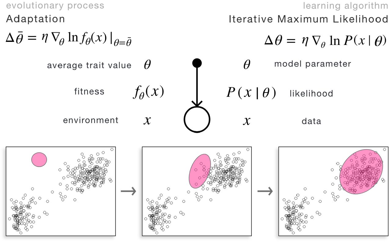
Left: on a microevolutionary timescale, replicator types are assumed to be fixed and their abundance is updated based on their fitness in the current environment. This is mapped to updating the probabilities of hypotheses based on how well they predict current data (i.e., their likelihood). Right: on a macroevolutionary timescale (right), mean phenotype of a population climbs the fitness surface, as a result of selection acting upon generated variation. This is mapped to gradient ascent on the likelihood surface. In both cases, the key ingredient is the identification of fitness of types over current environment with the likelihood of hypotheses over current data, depicted here as Gaussians.
Given the statistical structure of the environment and the constraint on possible fitness functions described above, replicator types compete to fit the environment in a manner analogous to the competition between hypotheses to predict the statistical structure of the data. Depending on the possible modes and timescales of adaptive mechanisms, minimal dynamical models of evolutionary processes map to different Bayesian models and inference procedures. In particular, two relevant timescales of evolution are i) microevolutionary timescale, where the change in abundance distribution over replicator types is explicitly modeled, ii) macroevolutionary timescale, where only the evolution of phenotypic population average is modeled. These are two complementary building block models of evolutionary dynamics, upon which additional ingredients, such as explicit mutation, ecological competition or multilevel selection, can be added. For simplicity, we refer to the former as selection and the latter as adaptation. Figure 1 illustrates these two elementary dynamics.
Selection, mutation, and adaptation
Selection by itself does not account for how variation is generated; instead, it assumes that replicator types are fixed and only their relative abundances pi(t) that change over time. Indeed, as described above, the abundance of those replicator types that fit the current environment x better increases at a higher rate according to the discrete-time replicator equation; equivalently, the posterior probability of those hypotheses that predict the current data better increase at a higher rate, described by Bayesian update. The corresponding graphical model is depicted in Figure 2. Whatever type/hypothesis had nonzero relative abundance/prior probability initially, only those types/hypotheses compete; no new types emerge. This dynamics is the simplest building block that models selection on a microevolutionary timescale.

Top: the graphical model corresponding to the replicator equation, describing selection over fixed types favoring types that are more fit in the current environment; and to Bayesian update, describing the change of probabilities of hypotheses, favoring hypotheses that predict current data better (i.e., have higher likelihood). Variables are illustrated by circles; (conditional) dependencies between them are symbolized by arrows. Bottom: Illustration of the process in a two-dimensional environment/data and Gaussian fitness/likelihood, depicted by ellipses. The phenotypes/hypotheses, characterized by the location, size, and orientation of the Gaussians, are fixed; their abundance/probability, signaled by the opacity of the ellipses, change according to how fit they are/how well they predict data.
Variation, generated by mutations, can be introduced into the selection-only model on two different timescales. The first approach extends the replicator equation by explicitly characterizing the number of mutation events, modeled by mutation rates µi←j from type j to type i. The evolutionary dynamics is therefore determined by the overall effect of two forces acting on the same timescale: selection and mutation. Mathematically, this simultaneous dynamics can be accounted for by the replicator-mutator equation (cf. eq. (2)),
 where µi←j determines the mutation probability (in unit time) from type j to type i and therefore is normalized as ∑iµi←j = 1, and the factor ∑kfk(xt)pk(t) is the average fitness of the population, responsible for keeping the distribution pi normalized at all times. Eq. (3) describes how fitness fi(xt) in the current environment, together with the mutation probabilities µi←j, update the abundance distribution pi. Similarly to the simple replicator equation, information about the environment is transferred to the abundance distribution over time; here, however, this information is filtered through the mutation probabilities, including the diagonal elements µi←i that specify the fidelity of replication. As observed by [14], this model of replication and mutation is equivalent to updating the probability distribution over latent hypotheses hi in hidden Markov models (HMMs). HMMs extend Bayesian update by introducing probabilistic transitions between hidden states (i.e. hypotheses) hi, and they infer the joint distribution {P (hi, t = 1), P (hi, t = 2), …, P (hi, t = T)} over the hidden states over time given data history {x1, x2 … xT}. In order to achieve this, HMMs need two quantities to be pre-determined: hypothesis hi’s likelihood of data, P (x|hi), just like in the case of simple Bayesian update, and the transition probabilities from hj to hi, denoted by P (hi|hj). This joint probability distribution over hypotheses at all times, {P (hi, t = 1), P (hi, t = 2), …, P(hi, t= T)}, can be reduced, however, to distributions of interest; if this distribution of interest is the one corresponding to the last timestep, P (hi, t), dynamically inferring this last distribution given data history is called the filtering problem in HMMs, and it is obtained through the dynamics
 that is indeed equivalent to eq. (3), with the identifications depicted in Figure 3. Importantly, HMMs can also be cast as Bayesian graphical models, illustrated also in Figure X. Note that this dynamics computes the predictive distribution at time t, corresponding to taking into account data until time t − 1 and transitions until time t; if data in the last timestep t is also integrated, eq. (4) needs a slight modification, corresponding to a less frequently used evolutionary counterpart.
The other approach of introducing the effect of mutations, that we refer to as adaptation, corresponds to modeling evolutionary dynamics at a qualitatively longer, macroevolutionary timescale. It does not explicitly account for mutations, instead, it assumes that a cloud of mutants in the (pheno)type space is always available upon which selection can act, irrespectively of what the generative mechanism of this variation is. It also shift the attention from tracking the abundance distribution of all types over time to simply following the population average of some relevant phenotypic traits. As an effect, in simple adaptive scenarios (with the explicit assumptions delineated below), the population average of relevant traits, denoted by  , evolves according to a gradient ascent on the (log) fitness landscape:
 where
where  is the change in the population average trait value (that can be a vector of any dimensionality), fθ(x) is the fitness of individuals with trait value θ given environmental state x, and η is the rate of adaptation. Indeed, the Price equation [16], in its simplest form (assuming no intergenerational transmission bias), relates the change in population average
  and the covariance between fitness and trait value cov(θ, f) as
  , where
  is the average fitness in the population. Assuming a deterministic fitness function fθ once the environment x is fixed, an isotropic cloud of mutants in the phenotype space, and that the variance in trait values is small enough to approximate the fitness linearly around the population average by
  , the Price equation implies (see Appendix) the dynamics given by eq. (5) with rate of adaptation being equal to the variance of trait values projected to the direction of fitness gradient, η = var(θ||).

Top: the graphical model corresponding to the replicator-mutator equation, describing the effect of selection and mutation among fixed types; and to hidden Markov models, describing the effect of Bayesian update in light of new data and transitions between fixed hypotheses. Bottom: the phenotypes/hypotheses are fixed, shown here by the fixed location, size, and orientation of the ellipses; their abundance/probability is driven by how fit they are/how well they predict data and by the mutation/transition probabilities between them.
This dynamics, assuming the above mentioned normalization constraint on fitness ∑xfθ(x) = 1, is equivalent to the gradient optimization of the (log) likelihood function,
 with learning rate η. The corresponding graphical model is shown in figure 4. Crucially, the connection between the two descriptions is given by the identification of fitness and likelihood again. In this model of macroevolutionary adaptation, new types can and do arise; however, it is only the phenotypic population average that this description accounts for. Furthermore, the rate of adaptation η is given by the phenotypic population variance that i) might change over time, and ii) is not modeled here, in accordance with the dynamical insufficiency of the Price equation [17].
Ecological competition
As we shall see, selection and adaptation, as well as the combination of the two, that is necessary to describe evolutionary-ecological interaction of species, form the basis of relating more complex evolutionary scenarios to their counterpart model within learning theories. One additional phenomenon relevant to life across all scales is competition for finite resources. Competition takes place at two timescales: on the ecological timescale, species abundances change according to their current ability to access the resources; on the evolutionary timescale, species themselves (i.e., their phenotypic average) become more adapted to the distribution of environmental resources in niche space. Ecological competition therefore serves as an important and, as we will see, the simplest nontrivial example in which combining dynamics at both timescales, referred to as selection and adaptation, is necessary. We model evolutionary-ecological dynamics as follows. Multiple species compete to access environmental resources; the amount of resources individuals of a species extract from the environment determines the abundance of the species. Mean phenotypic trait values of species and their abundances co-evolve. What makes the unfolding of these two dynamics non-trivial is that they are coupled: species adapt to the resources available to them, however, available resources are determined by the trait values of other species as well as their abundances. Abundances, set by the amount of resources species access, change according to the evolution of trait values of all species.

Top: the graphical model corresponding to macroevolutionary adaptation, i.e., the change in mean phenotype of a (quasi)species upwards in the fitness landscape, as a result of selection acting upon generated variation, neither of them is modeled explicitly here. It also describes how the parameters corresponding to a single hypothesis climb the likelihood surface to provide a better and better fit of data. Nodes (such as θ here) represent parameter(s), whereas circles represent variables. Bottom: adaptation of mean phenotype, depicted by the location, size, and orientation of the Gaussian, to the current environment. Equivalently, iterative optimization of the likelihood function to fit data.
Mathematically, we model the environment as a set of data points x1, …, xm, each of them corresponding to one unit of resource in resource space at their corresponding location within the niche space. Species i’s ability to access resource xj, depending on its trait value θi, is denoted by u(θi, xj). We refer to u as utilization. It is these trait values θ that species evolve, and therefore the adaptive trade-off any species face is imposed on their utilization function, ∑xu(θi, x) = 1, instead of on their fitness. Utilization determines how resources are divided: the share each individual of any species with mean phenotype θ receives out of resource j is proportional to its utilization at xj, u(θ, xj). Consequently, species i’s share of resource j, γij, is proportional to the product of its utilization u(θi, xj) and its relative abundance πi

The relative abundance πi of species i is, in turn, given by the total amount of resources its members access,

Relative abundances π and trait values θ co-evolve: relative abundances are updated given more adaptive trait values, whereas trait values evolve given the updated relative abundances. It is worthwhile to investigate how this model relates to a well-known model of ecological competition: the game-dynamical replicator equation. The continuous time game-dynamical replicator equation, describing ecological competition through abundance-dependent selection reads as  , where πi and fi is the relative abundance and fitness of type i, respectively, and
  is the average fitness. Importantly, in our model, quasi-equilibrium dynamics is assumed: trait values evolve on a timescale slow enough so that abundances are always in equilibrium given the current trait values. The equilibrium abundance distribution in the game-dynamical replicator equation (if exists), corresponds to all fitnesses being equal to the average fitness,
  for all types i. This can be satisfied by interpreting fitnesses as excess utilization values summed over environmental resources:
 where
where  . Indeed,
  for all i.
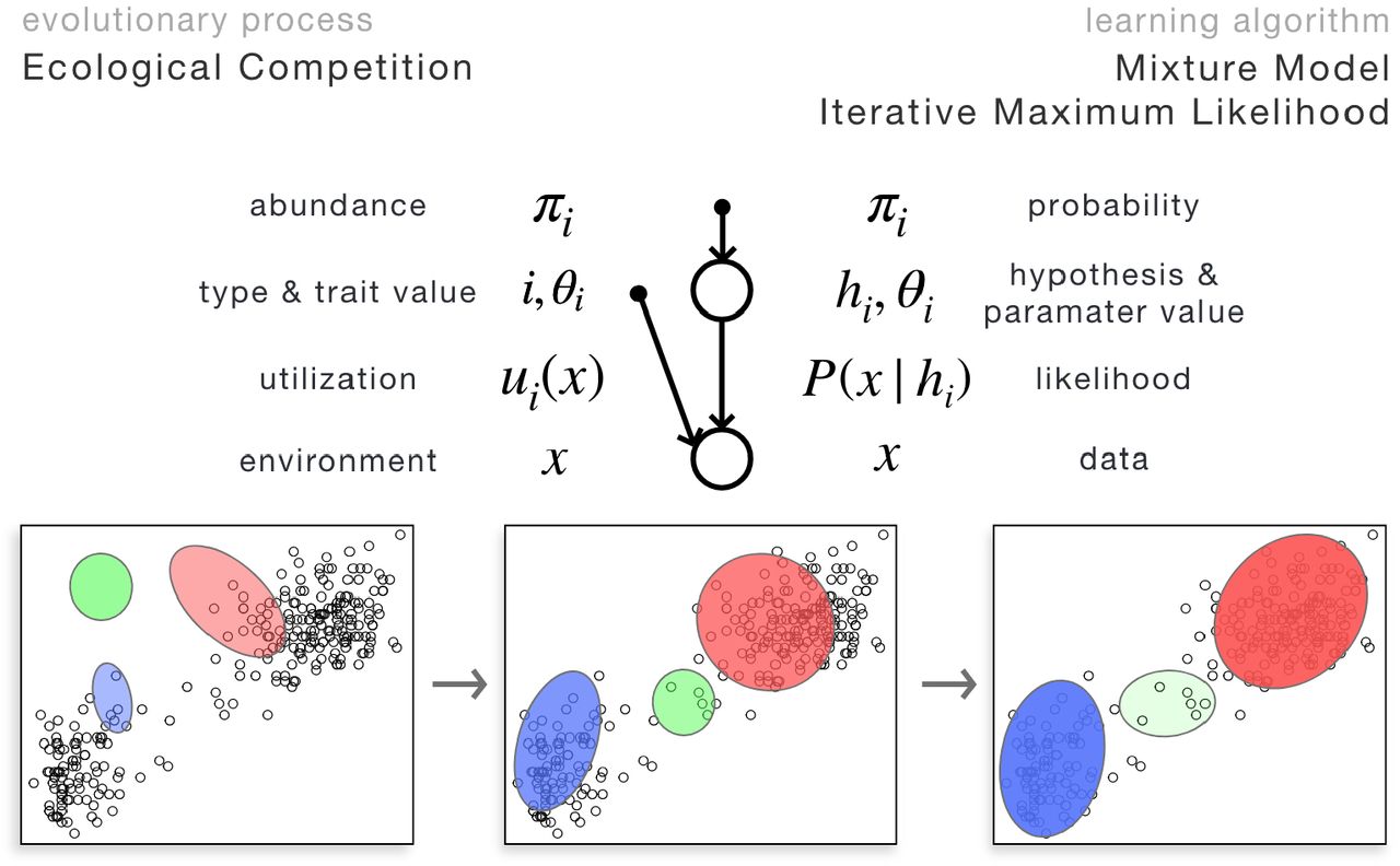
Interestingly, an equivalent formulation of this simple model of evolutionary-ecological dynamics, plays a central role in machine learning and Bayesian statistics: maximum likelihood estimation in mixture models via the expectation-maximization (EM) algorithm. Mixture models fit a weighted sum of distributions P (x) = ∑iP(x|{θi}, hi)πi to the data such that both the parameters of each component distribution {θi} and their relative weights {πi} are optimized in parallel improve on the likelihood of the whole model generating the actual data x. Since there is no known general closed-form formula for finding the global maximum of the likelihood function, in practice, mixture models are usually fitted iteratively using a variant of the expectation-maximization algorithm: parameters θi are improved given fixed weights πi, whereas weights πi are improved given fixed parameters θi; these two steps alternate until the parameters converge (assuming the data x does not change). Importantly, both the model framework (mixture models) and the dynamics (EM) are equivalent to the evolutionary-ecological dynamical model described above, with the following translation between the two interpretations: 1. species evolve their trait values θi to improve on their utilization function u(θi, x) and therefore extract more resources, corresponding to component distributions P (x|{θi}, hi) improving on their parameter θi to increase the overall likelihood of the model; 2. relative abundances πi are updated given the amount of resources that is accessible to a species, corresponding to updating the relative weights of the component distribution such that it increases the likelihood of the whole model.
One important message of this equivalence is that even though it is composed of competing agents, evolutionary-ecological dynamics, in this simple model, optimizes a global cost function, given by the likelihood of the counterpart probabilistic model. More generally, as many learning algorithm is based on iteratively optimizing a global cost function, finding such functions that are emergently optimized by evolutionary systems composed of competing agents is an important gateway towards a more unified discussion of evolution and learning. Finding a Lyapunov function (i.e., a scalar-valued function over the space of parameters on which the learning/evolutionary dynamics always follows a downwards path) is not always easy, finding one out of many possible ones that contributes meaningfully to a learning-theory based interpretation of emergent computations is even harder. In evolutionary theory, this line of thought goes back to Fisher’s fundamental theorem of natural selection, stating that a scalar function over (phenotypic) parameters, namely, average fitness, always increases if selection is not frequency-dependent [18]. It is perhaps less well known that a Lyapunov function always exists in frequency-dependent scenarios as well, now interpretable in the language of information theory: it is the Kullback-Leibler divergence (or relative entropy) between the current relative abundance distribution over types and the one at equilibrium that always decreases over time [19, 10, 20]. Following a similar path to find learning theoretically relevant Lyapunov/potential/cost functions in case of more complex dynamics of competing structures that are capable of representing patterns in high-dimensional data is a potentially important step towards a more unified theory of adaptation, incorporating both evolutionary systems composed of competing representations of the environment and learning systems that learn to represent data, many cases distributed over myriads of elementary computing units interacting only locally.
Another message the equivalence of this simple model of evolutionary-ecological dynamics and expectationmaximization in mixture models suggest is that it might be possible to engineer meta-level rules in synthetic evolutionary systems such that they learn as a whole to represent complex patterns in high-dimensional data. A further step towards designing creative artificial systems would be to build such an evolutionary system on complex-enough building blocks so that the complexification of representation can follow millions of diverging paths, impossible to list or foresee all of them by any existing technique, therefore rendering them unexpected and possibly creative.
Multilevel selection
When the replication of different replicator types are partially but not fully synchronized and groups of replicators inherit information regarding the identity of the group, an effective description of the system is provided by multilevel selection theory (MLS) [21]. MLS decomposes the full effect of selection hierarchically to selection acting between and within groups. Partially synchronized replicators form a necessary intermediate step towards new emerging units of evolution, i.e., transitions in individuality, that is, in turn, a main mechanism responsible for increasing complexity in evolutionary systems. Understanding MLS is therefore of crucial importance regarding any, natural or engineered, open-ended Darwinian system.
MLS acts on a hierarchical population of replicators: types of individuals hi are grouped into types of collectives zj. A complete static description of the population is given by the abundance and composition of collectives (for further details, see [15]). The composition of collective zj, denoted by  , normalized as
  , quantifies the relative abundance of individual level replicators within collectives of type zj. The total abundance of collective zj, measured as the total abundance of individual-level replicators within collectives of type zj, is denoted by pj and normalized as
  . These two sets of relative abundances, the compositions of collectives
  and their abundance, pj, describe the the composition of the hierarchical (two-level) population completely. From these two quantities, a third one, the total abundance of individuallevel replicators of type hi being part of collective zj, denoted by
  , can be calculated as
  . This quantity connects the two population levels in a sense that the abundance distribution of any level can be computed by summing over the other level: at the level of collectives, the abundance distribution, as we have seen, is given by
  ; at the level of individuals, the abundance of type hi, pi, is obtained by adding up the abundances of type hi being in any collective,
  .
.

Top: A simple model of evolutionary-ecological dynamics, including intra-species adaptation and inter-species competition for finite resources. Equivalently, this model also corresponds to fitting data with multiple component distributions through optimizing a global likelihood function. This model exemplifies evolutionary systems possessing a global cost (or energy) function that is interpretable in the language of learning algorithms. Bottom: Evolutionary-ecological dynamics of three species, or equivalently, iterative maximum likelihood (e.g., Expectation-Maximization) optimization of a model involving three component distributions. Each datapoint here corresponds to one unit of resources that is shared between species based on their utilization ability. This resource competition drives species to occupy separate niches, or equivalently, component distributions to avoid overlap. Species abundances (opacity) and their mean phenotype (location, size, and orientation of the Gaussian) co-evolve, driven by the amount of resources they access; equivalently, parameters of component distributions and their weights are iteratively optimized such that the global likelihood of the model is improved.
These quantities above describe the composition of the population at one time instance. How does selection change this hierarchical population over time? According to the discrete-time replicator dynamics, abundances change proportionally to their fitness. Here, however, the fitness of an individual-level type hi might very well depend on the collective zj it is part of; we denote this fitness by  . We also allow this fitness to depend on the environment x. The replicator dynamics, tracking the abundance of individuals of type hi being part of collectives zj, then reads as
 where the average fitness,
  , is calculated as
  . Tracking the abundance distribution at any level is then possible by summing over the other level, as discussed above. This, however, does not mean that the dynamics at the two levels are decoupled, for example, at the level of individuals,
  .
.
Crucially, fitnesses and abundances are assigned to types that connect the two levels, namely, to individuals of type hi that are part of collective zj. The replicator equation acts on these quantities, evolving the multilevel population in time. This conceptualization of MLS allows for relating multilevel evolutionary dynamics to hierarchical Bayesian computations over multivariate distributions: these two hierarchical dynamics are structurally equivalent, with the identified quantities listed in Figure 6. Note that this analogy can be extended to arbitrary number of levels, see [15] for details.

Bayesian inference in hierarchical models is equivalent to a model of multilevel selection. This identification relies on the possibility of representing multivariate probability distributions by hierarchical populations, combined with the equivalence of Bayesian update and discrete replicator equation.
An important aspect of multivariate Bayesian models is that it is possible to identify a parametrizationindependent backbone of the model in terms of conditional independence relations between variables. This allows for distinguishing between model structure (topology) and parameters, a necessary step towards modeling causality [22]. As discussed in [15], conditional independence relations imposed on the evolutionary implementation of the corresponding Bayesian model have a well-defined intuitive meaning, too: it corresponds to freezing compositions at various levels of the hierarchical population.
Another fundamental feature of hierarchical models is their complexity. Finding the probabilistic model with optimal complexity given data is a non-trivial task that can be approached from many directions. The Bayesian approach is to gauge the model’s performance averaged over all possible parameter settings of hidden variables [23]. When comparing two models, possibly having different number of variables and different number of hierarchical levels, one has to favor the one that predict data better on average. Interestingly, this Bayesian agenda translates to a general and simple evolutionary interpretation: if the average fitness of a collection of replicators is higher when they are grouped together in a collective compared to the case when they are “free”, a new level emerges. Although this model of evolutionary transition of individuality [24, 25] is rather simplistic in terms of dynamics, it is not in terms of structure, and we believe that this similarity is quite remarkable, having the potential to be refined later on to understand and design complexifying evolutionary systems.
3 Discussion
Bayesian models provide the recipe of performing i) consistent probabilistic computations such that ii) the system extracts the maximum amount of information from the environment given clearly specified model constraints. They therefore form a unique cornerstone of any adaptive dynamics in uncertain environments. Their power lies in their generality: the algorithmic and implementational details constrained by the given physical/informational substrate is not specified. Here we show that it is possible to implement many of the most relevant types of Bayesian computations by simple replicator-based systems. On top of the basic ingredients that include Bayesian update over one hidden variable and iterative optimization of cost surfaces (e.g., maximum likelihood, maximum a posteriori estimation at any level of the Bayesian hierarchical model), we attempt to provide guidance for replicator-based implementation of some fundamental building blocks of the full Bayesian apparatus, such as inference in mixture models, hidden Markov models and hierarchical models. What makes such a translation table especially appealing is the simplicity of such implementations on the evolutionary side: they do not require introducing fundamental conceptual novelties, instead they correspond to well-known dynamics such as models of ecological competition, mutation and multilevel selection. This observation hints at a more unified picture of evolutionary dynamics and probabilistic learning; but it might also provide a ground for transferring more advanced computational techniques from one field to the other. These, we believe, might include leveraging the parallel accumulation of rare subsolutions and of sex, the possibilities of maintained search for (more and more complex) novelties given by an open-ended replicator system, or, from the side of probabilistic computations, finding an emergent global cost function that is improved upon by the dynamics of competing replicating agents, explaining the seemingly paradoxical adaptive potential of evolutionary systems as wholes.
We envisage three aspects of human inquiry that potentially benefit from this correspondence between evolutionary and probabilistic computations.
First, to explain the adaptive potential of any Darwinian dynamics in Nature, both those that we already have plenty of observations and understanding about (Darwinian processes on a genetic basis), but also those that have not yet been fully acknowledged, and the usefulness of replicator-based modeling is questionable at this point, such as memetics [26, 27], Darwinian neurodynamics [28, 29] or quantum Darwinism [30]. Such explanations would mostly be based on either i) finding global cost functions that evolutionary system emergently optimize or ii) relating the computations performed by the system to probabilistic computations that optimally extract information from external data.
Second, many aspects of animal (including human) cognition is efficiently modeled by the framework of Bayesian inference and generative models. This is in line with selective pressures favoring optimal extraction of information about the environment that in turn enables to select action that leads to maximum survival and reproduction probability. The possible implementations of Bayesian computations on neural substrates, however, is not fully explored. Here we hint at one possible implementation, based on copying and evaluation of any neural information. We do not posit that all Bayesian computations are implemented this way, instead, we point at the possibility that the effective information extraction provided by Bayesian computations might be efficiently combined with the open-ended novelty generation evolutionary systems are capable of.
This leads to our third point: the possibility of leveraging the combination of evolutionary and Bayesian computations in designing future AI systems to generate creative yet optimally informed solutions/actions in any probabilistic environment. This direction would, in the very first place, need a more thorough understanding of the relation between evolutionary dynamics and learning theories, possible unified in the same mathematical language.
Appendix
Showing that the rate of adaptation η equals to the phenotypic population variance in the direction of fitness gradient, (θ||). In the following, cov, var, corr and std denotes covariance, variance, correlation and standard deviation, respectively. We assume for simplicity that the variance in trait values is small enough to approximate the fitness linearly around the population average by  , and we also assume for simplicity that the mutant cloud in the phenotype space is isotropic around the population average. Furthermore, it is also assumed throughout the paper that the mapping fθ(x) from trait values θ and environment x to fitness f is deterministic, implying that corr(f, θ) = 1. Since selection acts in the direction of the (log) fitness gradient ∇θ ln fθ(x), we project the trait vector θ into that direction, denoted by θ||. Applying the one dimensional Price equation to θ|| and using the identity |∇θfθ(x)|std(θ||) = std(f) and
  validated by the linear approximation of the fitness landscape, we obtain
  .
.


