

Abstract
Estimating effective population size, given a coalescent genealogy reconstructed from sequences that are longitudinally sampled from that population, is an important problem in epidemiology and macroevolution. Here the population represents infected individuals across a viral epidemic or historical abundances of a species of interest. The coalescent and sample times delineate the branches and tips of the reconstructed genealogy. Popular skyline estimators use these coalescent times to infer population size, but presume that sample times are predetermined and uninformative. We question this assumption, and formulate a new skyline method, termed the epoch sampling skyline plot (ESP), to rigorously incorporate sample time information. Our method uses an epochal sampling model in which the longitudinal sampling rate has a piecewise-constant, proportional dependence on population size, with constants of proportionality known as sampling intensities. We prove that the ESP can at least double the best precision achievable by standard skylines, while still fitting practical and flexible sampling scenarios. These include widely used density and frequency dependent protocols, which feature fixed sampling intensities, or constant sample counts. We show that sampling intensities, and population sizes can be jointly estimated, and that our estimates are markedly improved in periods where standard skyline methods are biased by long coalescent branches. We benchmark the ESP against existing approaches using simulated and empirical datasets, and provide efficient Bayesian (BEAST2) and maximum-likelihood implementations. Ignoring the sampling process disregards a rich source of information that could become increasingly important as data collection improves and intensifies.
I. Introduction
The coalescent process describes how fluctuations in effective population size influence the genealogical patterns of sequences sampled from that population (Kingman, 1982). In molecular epidemiology and macroevolution, where the coalescent process is widely used as a null model for diversity, the population usually represents the infected caseload in a viral epidemic or the abundance of an animal species. Sequences are sampled longitudinally (in time) across that epidemic (Pybus and Rambaut, 2009) or obtained from ancient DNA (e.g. fossils) that span the history of that species (Shapiro and Hofreiter, 2014). Estimating the effective population size from a coalescent genealogy that is reconstructed from those temporally sampled sequences (also known as a heterochronous tree), is an important and common problem.
The skyline family of inference methods (Strimmer and Pybus, 2001; Drummond et al., 2005; Minin et al., 2008; Gill et al., 2012), which are extensions of the classic skyline plot (Pybus et al., 2000), present popular, and prevailing solutions to this problem. These methods estimate a piecewise-constant population size profile using only the coalescent event times, which form the branching points of the reconstructed tree, and are inversely proportional to population size (Kingman, 1982). Sequence sampling times, which compose the tips of this tree, are thought to be preset by extrinsic factors such as historical surveillance programmes or operational capacities (Ho and Shapiro, 2011). As a result, skyline methods presume that sampling times are uninformative, and independent of population size (Drummond et al., 2005; Parag and Pybus, 2019).
Recent work has started to challenge this assumption, and assess its consequences. In Volz and Frost (2014), it was shown, for a coalescent process with exponentially growing population size, that including sampling time information could notably improve the precision of parameter estimates, provided that the sampling time process was correctly specified. This work recommended augmenting the coalescent process with a sampling time model, and defined a proportional sampling process, in which the sample rate at any time was linearly dependent on the population size at that time. This augmented model was generalised by Karcher et al. (2016) to include non-linear dependence, which they termed preferential sampling, and to allow for piecewise-constant population sizes. This study cautioned that misleading inferences could be obtained if preferential sampling, when present, is ignored, and is currently being extended to incorporate covariate models (Karcher et al., 2019).
While these works make noteworthy progress in evaluating and using sampling time information, their conclusions are based entirely on simulations and empirical observations. Consequently, they cannot provide provable or precisely quantifiable insights. Further, they do not explicitly consider the types of protocols likely to be practically implemented by collection centres, monitoring stations or surveillance programmes. Instead, they treat the sampling process as an additional, parametric model that is appended onto the coalescent process (Karcher et al., 2016). Here we attempt to resolve these issues by developing a new integrated sampling aware coalescent skyline model, which we term the epoch sampling skyline plot (ESP). The ESP presents a methodologically different approach. It reformulates the classic skyline plot to directly include a flexible epochal sampling model that can simulate practical scenarios.
This assumes that sampling occurs in epochs, which could approximate weekly or monthly surveillance cycles, epidemic half-seasons or specific fossil collection periods, among others. The boundaries of each epoch are delineated by the actual sample times of the reconstructed tree. This guarantees model identifiability and guards against unsupported inferences. For example, we cannot expect to estimate weekly sample rate changes from a tree with monthly tips. Within an epoch, sample times depend proportionally on population size, with a constant of proportionality that we call the sampling intensity. This intensity measures the average sampling effort over the epoch, with larger values corresponding to faster rates of sample accumulation. We allow the sampling intensity to change discontinuously between epochs. This results in a piecewise-constant sampling process that can flexibly fit many sampling protocols.
If we define a single persistent epoch, then we model density dependent sampling, in which the rate of collecting samples directly correlates with the effective population size. This is a common protocol, which posits that the availability of sequences depends on the size of the population to be sampled (Karcher et al., 2016). Density dependent protocols result in a fixed proportion of the population being sequenced per time period. If instead, we define many epochs uniformly across time, and adjust the sampling intensity within each epoch to produce an approximately equal number of samples per epoch, then we obtain a frequency dependent sampling strategy. This strategy models practical, extrinsic limitations to sampling effort, such as surveillance capacity (Ho and Shapiro, 2011), and results in a fixed number of sequences being sampled per time period, irrespective of population size. This protocol gives a snapshot of the genetic diversity within the population during each epoch, and is used, for example, to monitor various strains of an infectious disease.
We develop the epoch sampling skyline plot in New Approaches, and then demonstrate how to jointly estimate population size and the epochal sampling intensities in Results, within both maximum likelihood and Bayesian frameworks. There we also benchmark the ESP against existing skyline techniques using both simulated and empirical epidemic data (seasonal influenza in New York state and steppe bison in Beringia). In particular, we model and infer under practical density, and frequency dependent sampling protocols, to illustrate the efficacy of the ESP. We show that the counteracting proportional and inverse dependencies in our skyline especially improves estimates in periods where standard skylines are biased by long coalescent branches. We quantify and guarantee these improvements by proving that the information available for estimating population size (and hence the best precision of these estimates) can more than double by including the epochal model. In Materials and Methods we examine further theoretical properties of our skyline and detail its maximum-likelihood and Bayesian implementations. The former is available on GitHub, while the latter is provided as an integrated package in the popular software BEAST2 (Bouckaert et al., 2019).
II. New Approaches
Consider a coalescent tree reconstructed from sequences sampled longitudinally along an epidemic or from fossils spanning a period of interest. Let the effective population size underlying this process at time t, into the past, be N(t). Standard coalescent skyline approaches to estimating N(t) assume that sequence sample times are uninformative (Drummond et al., 2005), and so draw all of their inferential power from the reconstructed coalescent time series. These methods approximate N(t) with a p segment piecewise-constant function:  , with tj – tj−1 as the duration of jth segment and 1𝔸(x) as an indicator variable, which is 1 if x ∈ 𝔸 and 0 otherwise, for some set 𝔸. Here t0 = 0 is the present. Fig. 1 illustrates a coalescent sub-tree spanning the jth segment, with population size Nj. Two epochs with intensities β1 and β2, occur within this segment. Observe that coalescent event times (grey) form the branching points of this tree, while sampling events (cyan) control when new tips are introduced.

Schematic of epoch sampling skyline. A temporally sampled (heterochronous) tree consists of sampled tips and coalescing branches. A portion of this tree over the jth segment where effective population size is assumed to be fixed at Nj is shown (top). Our epoch model assumes a piecewise constant sample intensity function comprising two epochs over this tree segment (middle). The sampling times (cyan), inform on these epoch intensities (and determine the epoch boundaries) while the coalescent event times (grey) allow inference of Nj (bottom) (and control the segment changes). See New Approaches for definitions of the mathematical notation used.
We use Δi to measure the duration of the ith inter-event period or interval within this segment, and define the lineage count in this interval a. If there are k intervals in the jth segment then  . We use the sets 𝕊 and ℂ to indicate whether an interval ends with a sampling coalescent event respectively. Then
  and
and  count the number of sampling and coalescent events in this segment, and k = s + c. Note that s, c and k are not fixed, and can have different values for all p segments. Events which occur at a change-point belong to the interval that precedes that change-point (hence the sampling events 1𝕤 (2) and 1𝕤 (3) belong to the first epoch, and the starting two lineages are included in the likelihood of the (j – 1)th segment).
Coalescent events falling within this segment follow a Poisson process with rate  with
with  , and Nj, as the un-known population size parameter (Kingman, 1982). As a result,
  describes the key informative relationship in coalescent processes. Standard skyline methods capitalise on this dependence, but assume that intervals that end in sampling events are uninformative. These are the {Δi: i ∈ 𝕊}. Under this assumption the maximum Fisher information, about Nj, that can be extracted by these methods is
  (Parag and Pybus, 2017).
Our approach instead posits that the sample times within the ith interval of the jth segment derive from a Poisson process of rate βiNj. Here βi is the sampling intensity governing the sampling effort made across Δi. This encodes the extra informative relationship: βi Δi ∼ exp(Nj), and is the most complex sampling model that can be included within the skyline framework. We remove unnecessary complexity from this model by defining epochs as consecutive sets of intervals (which may span different segments) over which the sampling intensity is constant. Thus, within an epoch all βi take the same value (in Fig. 1 βi for i ≤ 3 are all set to β1). Epoch change times are assumed to coincide with sample times, and the sampling intensity is set to 0 beyond the last sample, where the ESP reduces to a standard skyline model. Our description ensures that each skyline segment, and epoch has at least one coalescent, and sampling event, respectively. This guarantees that the ESP is maximally flexible, yet statistically identifiable (Parag and Pybus, 2019).
Our epochal model, unlike previous attempts at incorporating sample times (Volz and Frost, 2014; Karcher et al., 2016), accounts for the discreteness of practical sampling protocols (sampling often occurs in bursts with discontinuous sampling effort changes between collection periods), and does not assume any long-term parametric relationship between sampling and the infected population (epochal sampling intensities are independent of one another). Using this framework we construct the ESP log-likelihood for the jth segment, ℒj = log P(𝒯 | Nj), as in Eq. (1), with 𝒯 as the reconstructed tree.

The complete log-likelihood is then  . The waiting time until the end of any interval contributes
  , while sampling and coalescent events introduce the 1𝕤 (i) log(βiNj) and
  terms, respectively. Eq. (1) is related to the augmented log-likelihood from Karcher et al. (2016), but differs in both the population size and sampling models used. If we define p′ epochs over 𝒯, then there are p + p′ unknown parameters in our log-likelihood (the set of Nj and distinct, non-zero βi).
The epoch sampling skyline is obtained from Eq. (1) by com-puting the grouped maximum likelihood estimate (MLE),  . It involves solving a pair of quadratic equations that depend on the relative number of sampling and coalescent events in that segment, s – c (see Material and Methods). Defining
  and
and  , we obtain Eq. (2), from the roots of these quadratics.

Eq. (2) forms our main result. In practice, since the MLE of each  , is jointly estimated, we usually replace b with
  . If s = c, both parts of Eq. (2) converge to the simple square root estimator,
  . Grouping over k adjacent intervals in our skyline leads to improved population size estimates that are quick to compute and easy to generalise. Note that if s = 0, and c = 1 then Eq. (2) recovers the classic skyline plot (Pybus et al., 2000).
The ESP has several important and desirable properties. Its counteracting proportional and inverse dependencies mean that it has more informative intervals in regions where long coalescent branches would generally hinder standard skyline inference. This spreads the information more uniformly across the time period of investigation. Moreover, it provably improves overall estimate precision (see Results). The Fisher information the ESP extracts from the same reconstructed tree is now at least  , for the jth segment. Thus, whenever the number of sampling and coalescent events are roughly equal, our best attainable asymptotic precision (which is the inverse of the variance), at minimum, doubles.
III. Results
A. Simulated Performance
We start by comparing the solution of Eq. (2) to the classic skyline plot from Pybus et al. (2000), which ignores sampling dependencies, and is the basis for all popular standard skyline methods. We keep the number of piecewise-constant segments inferred (model dimensionality) roughly the same by fixing k = 2 in the ESP. Here we assume a single, known sampling intensity for clarity, and only examine the period until the last observed sample time (into the past). Beyond this point, the sampling model is inactive. We demonstrate the relative ability of both methods to recover different population size dynamics in Fig. 2a–Fig. 2c. In these plots the top panel is the classic skyline, the middle panel is the ESP at k = 2 (for the same, fixed sampled tree), and the bottom panel gives the distribution of sampling (cyan) and coalescent (grey) events.

ESP performance. Panels (a)-(c) compare the classic skyline (top) to the ESP at k = 2 (middle) for exponential growth, cyclical logistic growth and steep periodic dynamics. Here the skylines are in cyan and the true demographic function (to be inferred) in dashed black. The classic skyline fails when the population size is large (a), or when there are notable fluctuations between large and small populations (b-c). This results from the uneven clustering of coalescent events (grey in bottom). The sampling events (cyan in bottom sub-panels) are inversely distributed to the coalescent ones and so the ESP has more evenly spread information throughout these demographic functions. Consequently it achieves better tracking, for the same number of population size segments. Panel (d) shows how increasing the grouping, k, can improve the smoothing of the ESP for a bottleneck demographic function. All trees were simulated using the phylodyn R package (Karcher et al., 2017) with approximately 300 coalescent and sample events.
The ESP significantly improves inference. It provides much better estimation in periods of large population size (Fig. 2a), and can handle sharp changes (Fig. 2c). Standard skyline approaches are known to fail in these cases because coalescent branches are too long, making their estimates unreliable or inflexible. Further, coalescent events usually cluster around bottlenecks (Fig. 2b), causing standard methods to lose fidelity across cyclic epidemics. Epochal sampling events, however, fall in periods of sparse coalescence, thus allowing the ESP to circumvent these classically problematic conditions.
Due to the noisy nature of the classic skyline plot, the generalised skyline was introduced in Strimmer and Pybus (2001). It grouped intervals to achieve a bias-variance trade-off that led to smoother estimates. This grouping is at the core of some popular skyline approaches (Drummond et al., 2005). We can achieve a similar effect in our skyline by increasing the grouping parameter, k (see Fig. 2d). This extends the generalised skyline to include knowledge of the individual events within a group, and to allow for sampling.
Having clarified the attributes of our skyline we now examine more practical examples, where the sampling intensities are unknown. We assume that the times corresponding to all sampling events are avail-able. In this work we consider two realistic, and widely used sampling protocols, which we respectively refer to as density dependent, and frequency dependent. Density dependent sampling models a direct correlation between the time-varying effective population size and the sampling rate. It features a single sampling intensity over an epoch that persists throughout the complete sampling period, and is the simplest model described within our epochal framework.
In practice, health bodies or treatment centres may provide a relatively fixed number of samples over some recurrent, longitudinal interval of an epidemic (e.g. seasonal case counts). This number could be constrained by extrinsic factors such as surveillance or sequencing capacity. Similar constraints may control the availability of ancient DNA sequences in macroevolutionary studies, though these are likely to be more random in time. In these cases, due to underlying changes in the demographic function, the sampling intensity is also effectively time-varying. The frequency dependent sampling protocol models this scenario, which explores the full complexity of our epochal model. Given its extra complexity, we only examine frequency dependent sampling under our fixed tree maximum-likelihood approach as a proof of concept. Later, we will provide detailed analyses of both schemes (with comparisons to popular skyline approaches) using our Bayesian package in BEAST2, which samples across group sizes and accounts for genealogical uncertainty (see Materials and Methods).
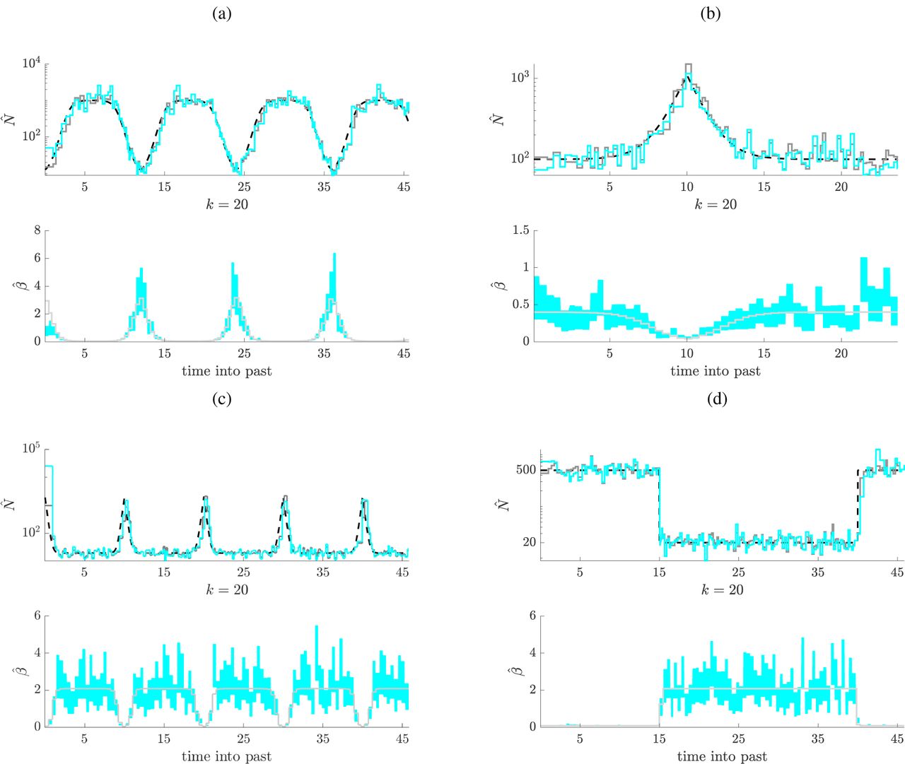
We define our sampling protocol as having p′ epochs. Hence there are p′ unknown sets of βi values to infer (within each epoch all βi take the same value). We use β to represent this vector of unknowns, and let its MLE be  . Note that epoch and population size change-points do not need to be synchronised, and we are jointly estimating a total of p + p′ parameters. Fig. 3a–Fig. 3d present our joint estimates of N and β at k = 20 for several test epidemic scenarios with frequency dependent sampling at p′ = 100 (Fig. 3a and Fig. 3c) or p′ = 50 (Fig. 3b and Fig. 3d). Since sampling is uniform across epochs, β takes a complimentary form to the population size fluctuations. In the
  plots (top panels) the dark grey represents the ESP with known β and the cyan is the jointly estimated ESP under the MLE
  (see Eq. (2)). In the
  plots (bottom panels) the true β is in grey while the estimated 95% Fisher information based confidence intervals
  , see Materials and Methods) are in cyan. We faithfully reproduce changes in both the population size and sampling intensity, demonstrating the power of the ESP.

Joint population size and sampling intensity inference. Panels (a)-(d) examine ESP population size (top) and sampling intensity (bottom) estimates under frequency dependent sampling for cyclical logistic, boom-bust, steep periodic and bottleneck dynamics. Simulations (a) and (c) use 2000 samples over 4 cycles with p’ = 100 and k = 20, while (b) and (d) use 1000 samples with p’ = 50. In the top sub-panels the joint ESP population size estimates (cyan) are compared to the true demographic function (dashed) and the ESP with known sampling intensity. The bottom sub-panels show the ESP intensity estimates (cyan) with their 95% Fisher information confidence intervals against the true sampling intensity (grey).
B. Bayesian Simulation Study
Having explored the performance of our maximum likelihood ESP, we now investigate and validate our Bayesian implementation, which we call the BESP. The BESP incorporates the ESP log-likelihood within the powerful computational framework of BEAST2 (see Materials and Methods). Here we benchmark the ability of the BESP to recover accurate and unbiased parameter estimates. We simulated 100 replicate coalescent genealogies (using the phylodyn R package (Karcher et al., 2017)) under (1) constant-size, (2) bottle-neck, (3) boom-bust, (4) cyclical boom-bust and (5) logistic growth and decline population size trajectories (N (t)). In all simulations we used frequency dependent sampling with roughly equal numbers of samples split over 24 equidistant sampling epochs. We used fixed trees to avoid confounding noise from genealogical uncertainty due to substitution model parameter and tree topology estimates, and jointly inferred N and β from each replicate fixed tree via the BESP.
In all inferences we grouped coalescent and sampling events into p = 100 equally informed population size segments (i.e. k is equal for all segments) to estimate N and used p′ = 24 roughly equidistant sampling epochs for β. We assessed the BESP by computing the relative bias, relative highest posterior density (HPD) interval width and coverage, averaged across its inferred N or β between the most recent and oldest samples. Together, these statistics allow us to quantify the bias and precision of the BESP estimator. Further details on the simulations, inferences and summary statistics can be found in the supplementary material. The results of our simulation study are given in Fig. 4. Example replicate trees and inferred trajectories are provided in Fig S1-S5.

Standard boxplots and stripcharts for the mean relative bias, mean relative HPD interval and mean coverage for the population size (N) and sampling intensity (β) estimates inferred from 100 replicate simulations across 5 scenarios. Statistics were averaged across parameter estimates from the most recent to the oldest samples.
Both N and β are slightly overestimated, with a somewhat larger bias in the β estimates. Nonetheless, the boxplots for the mean relative bias intersect 0 for all 5 simulation scenarios, verifying good tracking accuracy. The mean relative HPD interval widths of the population size estimates are below 2 (the width under a Gaussian approximation with standard deviation equal to the absolute value of the parameter is approximately 3.92) for all replicate cases, with only a few outliers under the logistic and boom-bust scenario. The boom-bust case features β estimates with mean HPD interval widths greater than 2, but only for a few replicates. This is a consequence of the BESP not having enough power for precise estimates of β during the most recent sampling epoch under boom-bust dynamics (see Fig. S3). Relative HPD intervals smaller than 2 indicate that estimates are at least twice as precise as a standard Gaussian approximation. Lastly, the mean coverage is always close to 1, indicating that the true N and β are both included within the HPD intervals for the majority of the sampling period. In combination, these results validate the low bias and high precision of the BESP approach.
C. Case Study 1: Seasonal Influenza
Seasonal influenza causes yearly epidemics during winter in tem-perate regions. Strong selective pressures on receptor and antibody binding sites of the surface glycoprotein haemagglutinin (HA) drives antigenic drift, which results in the continuous replacement of circulating strains with new variants (Ferguson et al., 2003). This constant emergence of novel genetic strains able to re-infect hosts immune to earlier strains causes a significant public health burden (Heester-beek et al., 2015). Among circulating subtypes, influenza A/H3N2 dominates most years, causes the most synchronous outbreaks and is associated with the highest morbidity and mortality (Viboud et al., 2006). Rambaut et al. (2008) used 1,302 complete A/H3N2 and A/H1N1 viral genomes sampled from temperate regions to show that a source-sink model provides a plausible explanation for seasonal influenza dynamics.
In this model strains re-emerge annually from a tropical source population and then, through global aviation networks, seed winter epidemics in temperate sink regions. In virus genomes sampled from temperate regions the interplay between strong selection on surface antigens and global travel networks manifests as an exponential increase in genetic diversity at the start of each flu season, followed by a bottleneck at the end of that season. Rambaut et al. (2008) found that the Bayesian skyline plot (BSP), which ignores sam-pling information, can recover this pattern from A/H3N2 genomic sequences. Subsequently, Karcher et al. (2016) demonstrated, via a preferential sampling model, that these population size estimates could be improved by incorporating sampling time information.
We extend the analysis of seasonal influenza by using our BESP approach to investigate variations in the sampling intensity between seasons. Our dataset comprises 637 HA sequences of 1,698 bp from New York State that were previously examined in Rambaut et al. (2008). These sequences were originally extracted from the National Center for Biotechnology Influenza Virus Sequence Database and rep-resent 12 complete influenza seasons, from 1993/1994 to 2004/2005. We use the BESP with p = 40 population size segments and p′ = 12 sampling epochs, with each epoch roughly corresponding to the duration of one influenza season.
We compare our results to the BSP and an additional BESP with density dependent sampling i.e. a single, perennial sampling intensity. Note that while the population size parameter of the BESP, N, is proportional to the effective population size in the absence of natural selection (N = Neτ where τ is the average generation time), this does not hold for influenza, where strong directional selection exists. Instead, we interpret N as a measure of relative genetic diversity, as in Rambaut et al. (2008). Here we directly infer our estimates from the sequencing data, while incorporating phylogenetic uncertainty. All substitution and clock models we employ are in keeping with Rambaut et al. (2008). Further model details can be found in the supplementary material.
Fig. 5A shows that considerably fewer samples in the dataset originate from the 1995/1996, 2000/2001 and 2002/2003 influenza seasons. This is consistent with independent epidemiological surveillance data, which shows that none of these seasons were dominated by A/H3N2 (Goldstein et al., 2011; Ferguson et al., 2003). The inferred genetic diversity trajectory (Fig. 5B) is highly synchronous, with peaks at the midpoint of each season, except 2000/2001 and 2002/2003. The complete absence of a peak in 2000/2001 agrees with surveillance data, as almost no A/H3N2 cases were reported that season (Goldstein et al., 2011). On the other hand, the BESP infers a small, somewhat later peak for the 2002/2003 season. Surveillance data indicates that while 2002/2003 was very mild and dominated by a mixture of A/H1N1 and B, a substantial proportion of A/H3N2 cases were reported toward the end of that season (Goldstein et al., 2011). Finally, while the 1995/1996 season was predominantly A/H1N1, around 40% of influenza incidence was still attributed to A/H3N2 (Ferguson et al., 2003). This explains why the epidemic peak inferred for this season is as high as those with only A/H3N2 cases (see Fig. 5B).

(A) Sample density through time for the 637 HA sequences used in the example. Red shading shows the kernel density estimate, blue dots indicate stripcharts of individual samples for each season. The height of the strip chart for each season is proportional to the sample density. Grey shading indicate the approximate period of influenza observation in New York state during each season (MMWR week 40 to week 20 in the next year). Cross-hatched seasons indicate seasons when A/H3N2 was not the dominant subtype. (B) Median and 95% HPD intervals of the genetic diversity estimates (Neτ) through time with the BESP (blue) and BSP (red). (C) Median and 95% HPD intervals of the sampling intensities (β) estimated for each sampling epoch with the BESP.
Although the the bottleneck level varies in some years (notably it is higher during 2002 and lower during 1997), this variation is not substantial and is less visible in absolute size (see Fig. S6). It appears that the bottleneck level largely depends on the availability of data since, in the absence of coalescent and sampling events, the smoothing prior maintains a roughly constant population size estimate (Volz and Frost, 2014). The strong bottleneck at the tail of each season ensures that individual A/H3N2 HA sequences contain almost no information about the genetic diversity of previous seasons. Thus, the informative events during a given influenza season almost all stem from sequences sampled in that season. This results in a ladder-like genealogy and explains why the BESP reveals no information prior to 1993/1994.
In comparison to the BESP, the BSP does not infer epidemic peaks in the 1996/1997 and 2002/2003 seasons (Fig. 5B). It also infers substantially smaller peaks in several other seasons. As observed above, we expect peaks for 1995/1996 and 2002/2003. The remaining seasons with lower/no peaks were all dominated by A/H3N2 (Ferguson et al., 2003; Goldstein et al., 2011). In particular, the 2003/2004 epidemic was more severe than usual and exclusively composed of A/H3N2. Thus, we conclude that the BSP does not have sufficient power to infer all epidemic peaks. Moreover, the BSP does not show sharp decreases in genetic diversity at the end of influenza seasons. This agrees well with simulation results, since coalescent events tend to be sparse during periods of large population size (at the start of a bottleneck), but sampling events are plentiful (see Fig. 2b). Unlike the BESP, the BSP cannot exploit these informative sampling events and fails to detect bottlenecks at the end of influenza seasons.
The inferred β for each season is shown in Fig. 5C. Except for the 2000/2001 season (during which almost no A/H3N2 cases were sampled), the 95% HPD intervals of all other seasons intersect. There is some variation in the median estimates, with larger uncertainty associated with the estimates for these years. The genetic diversity trajectory inferred by a simpler model with density dependent sampling almost matches those of the 12-epoch model above (see Fig S7). Further, the estimated sampling intensity of this simpler model passes through the HPD intervals estimated for all epochs except the 2000/2001 season and is roughly equal to the average intensity estimated from the 12-epoch model. We conclude that modelling differences in the sampling intensity through time is inconsequential to genetic diversity estimates. This is therefore an example of density-dependent sampling.
D. Case Study 2: Steppe Bison
The demographic history of the steppe bison, which exhibits boom-bust dynamics, is often used to validate the fitting performance of skyline methods (Shapiro et al., 2004; Drummond et al., 2005; Gill et al., 2012). Before the extinctions of the Late Quaternary period, Beringia (eastern Siberia across the Bering land bridge to Alaska and northwestern Canada), supported a large diversity of megafauna with the biomass dominated by bison, horses and mammoths. The large and diverse population of bison, along with favourable climatic conditions for specimen preservation means bison fossils suitable for ancient DNA extraction are abundant across Beringia (Shapiro et al., 2004). Modern molecular methods and radiocarbon dating allow the isolation and sequencing of ancient DNA from these fossils and can date specimens up to 55,000 years old with high confidence (Shapiro and Hofreiter, 2014). These techniques permit the reconstruction of time-stamped genealogies, which offer high-resolution reconstructions of demographic history.
The dataset we use is the same as in Gill et al. (2012) and consists of mtDNA control region sequences from 135 ancient and 17 modern bison samples, with the oldest sample dated 55.182 thousand years before present (ka BP). We treat sampling dates as known and use the BESP to infer the effective population size trajectory and sampling intensity through time with p = 20 segments, and p′ = 12 epochs. Each epoch lasts approximately 5000 years, except for the most recent, which stretches from the present to 450 years ago. We compared our results to a BSP with 20 population size segments, and a simpler density dependent BESP with a single sampling intensity. We adopt an HKY substitution model and use a strict molecular clock. Further model details can be found in the supplementary material.
Fig. 6A shows that the sample density is roughly constant through time, except for the most recent sampling epoch (0–450 years BP), which contains the most samples, and a period between 17 ka BP and 22 ka BP, which contains only 3 samples. This period coincides with the last glacial maximum (LGM) and Shapiro et al. (2004) reports that fossils from this time period are sparse. This extrinsic constraint meant that DNA could only be amplified from a few samples. The N and β estimates through time are shown in Fig. 6B and C, respectively. For comparison, the estimates of N under the BSP are also presented in Fig. 6B. We observe a persistent and sustained growth until a population peak around 45 ka BP. A rapid decline to a population bottleneck around 12 ka BP then follows, with a slight recovery in the recent past.

(A) Sample density through time for the 152 bison mtDNA sequences used in the example. Red shading shows the kernel density estimate, blue dots indicate stripcharts of individual samples for each sampling epoch. The height of the strip charts are proportional to the sample density during an epoch. Grey shading indicate cool periods in the Earth’s climate, from the present, Younger Dryas and Marine Isotope Stages (MIS) 2 and 4. The two cross hatched areas indicate the time of the last glacial maximum (LGM, ≈26.5–19 ka BP) and the time of human settlement of the Americas (≈16–14 ka BP). (B) Median and 95% HPD intervals of the genetic diversity estimates (Neτ) through time with the BESP (blue) and BSP (red). (C) Median and 95% HPD intervals of the sampling intensities (β) estimated for each sampling epoch with the BESP.
Both methods result in similar N estimates, with largely overlap-ping HPD intervals. However, the BESP features a more complex and rapid decline. Further, the BESP recovers a period with stable effective population size, intersecting with the LGM, before the final crash to the population bottleneck. Estimates of β vary across 4 orders of magnitude between the most recent and oldest samples. In particular, there is an order of magnitude difference between the present (0–450 BP), the period from the population bottleneck to recovery (450– 14,753 BP) and the stable population size period from the LGM to the crash (14,753–24,762BP). Prior to the LGM β steadily decreases to a minimum around the time of the population peak. During this period, comprising the oldest 6 sampling epochs, the sampling regime is roughly frequency dependent and, as in Fig. 3, the β estimates mirror N.
Using a simpler BESP with density dependent sampling leads to N being overestimated by an order of magnitude after the LGM, as compared to the BSP and the frequency dependent BESP (see Fig S8B). This implies a sudden exponential growth in the bison population after the LGM, with the population at its largest at present. These results are an artefact of the inflexible β estimate under this model (Fig S8C). Here enforcing a constant sampling intensity results in a vast underestimation of sampling effort in the period following the LGM. This in turn engenders spuriously large effective population sizes. Thus, while the BESP with 12 epochs has enough flexibility to compensate for changes in the sampling intensity, the BESP with constant sampling intensity cannot, and infers biased estimates. Similarly, the BSP makes no assumptions about the sampling model and infers an unbiased result with slightly more uncertainty than the BESP with 12 sampling epochs. It is likely that phylogenetic uncertainty masks any dramatic gains in precision that infromative sampling could afford here.
E. The Information in Sample Timing
Having demonstrated the benefits of the ESP, we provide theoreti-cal justification for its improved performance. While sample times are known to provide a potentially rich source of additional information (Volz and Frost, 2014), this idea has never been exactly or explicitly quantified in the literature. Here we apply the Fisher information approach from Parag and Pybus (2019) to assess the ESP against all standard skyline estimators, and to evaluate the benefits of integrating sampling with coalescent events. As in New Approaches we consider the part of the reconstructed tree that spans the jth population size, Nj, and contains s sampling and c coalescent events. We use Fisher information because it delimits the maximum asymptotic precision attainable by any unbiased estimator of Nj, such as the MLE (Kay, 1993). This precision defines the inverse of the variance around that estimator. The Fisher information is computed as the expected second derivative of the log-likelihood function (see Materials and Methods).
Popular skyline inference methods such as the Bayesian skyline plot (BSP) (Drummond et al., 2005), the Skyride (Minin et al., 2008), and the Skygrid (Gill et al., 2012) are all based around the log-likelihood ℒj, c, given in Eq. (3).

This only considers the c coalescent events to be informative about Nj. The specific log-likelihoods of these skyline methods can be obtained from Eq. (3) by simply altering either its population size or interval grouping procedure. Standard skyline estimates are then the MLEs of Eq. (3) or some related Bayesian variant. This gives the left side of Eq. (4), which modifies the grouped generalised skyline estimates of Strimmer and Pybus (2001) to cases where individual event times (within that group) are known.

The Fisher information, Ic(Nj), under these various skyline approaches, however, is identical and given by the right side of Eq. (4) (Parag and Pybus, 2019). The maximum precision (minimum variance), around  , achievable by all of these methods, is then its reciprocal, Ic(Nj)−1 (Kay, 1993).
We define a sampling equivalent to these skyline approaches, which completely ignores the coalescent event information in Eq. (5).

This log-likelihood assumes that only the s epochal sampling events are informative. The MLE and Fisher information follow in Eq. (6).

Interestingly, the per event Fisher information in this sampling equivalent model is exactly the same as that from any standard skyline method. This result explains and quantifies the assertion from Volz and Frost (2014) that N (t) can sometimes be estimated using just the sample time information.
Having considered its component information sources, we now examine the ESP, which considers both s sampling and c coalescent events to be informative. Using Eq. (1) we compute the Fisher information of the jth segment, I(Nj). This gives the revealing expression in Eq. (7), with grouping factor  .
.

Intriguingly, I(Nj) ≥ Is(Nj) + Ic(Nj). This means that we gain additional precision by integrating both sampling and coalescent models (the per event information has increased). This extra information comes from the counteracting proportional and inverse dependencies. Further, any segment with equal numbers of sampling and coalescent events, can now be estimated with at least twice the precision of any standard skyline approach, for the same reconstructed tree 𝒯. Since n sampled sequences lead to n − 1 coalescent events, and the total Fisher information is  , then the overall asymptotic precision across 𝒯 is roughly, at minimum, doubled.
This justifies and underpins the marked improvements in population size inference that the ESP achieved. However, this effect can sometimes be clouded by other sources of uncertainty such as genealogical error and disappears when the sampling times actually contain no information about population size (where the ESP converges to a standard skyline). An important consequence of this analysis is the explicit dependence of estimate precision on the number of events informing that estimate i.e. c for standard skylines, s for their sampling equivalent and s + c for the ESP. This suggests that whenever the number of informing events in a skyline segment is small, estimates of that segment should be disregarded (when this number is 0 the skyline is unidentifiable). We recommend identifying and excluding such regions from population size estimates as a precaution against misleading and overconfident inference.
The log-likelihood of Eq. (1) also provides power for inferring the sampling intensities across time (the βi parameters). The MLE and Fisher information provided by 𝒯 about βi over the duration of the jth population segment are given in Eq. (8).

The MLE depends on Nj, and thus has to be jointly estimated. The algorithms used to solve this problem are described in Materials and Methods. The Fisher information shows that only intervals ending with sampling events offer the power to estimate a sampling intensity parameter. This corresponds to the most flexible sampling model possible. Our epochs group across the βi so that the power for estimating an epochal sampling intensity depends on the total number of sampling events within that epoch. Since by definition each epoch has at least one sampling event, statistical identifiability is guaranteed (Parag and Pybus, 2019). Observe that our ability to infer these unknown piecewise-constant sampling parameters is exactly analogous to that of standard skyline approaches with respect to population size. Similarly we recommend ignoring epochs featuring a small number of sampling events.
IV. Discussion
The epoch sampling skyline plot or ESP is a practically motivated, yet theoretically justified approach to demographic inference under temporally sampled, coalescent genealogies. By exploiting both proportional, and inverse-proportional piecewise-constant dependencies, it can potentially and provably double the best achievable precision of our effective population size estimates. Moreover, it facilitates the flexible inference of hidden, time-varying sampling intensities that modulate realistic data collection protocols. It presents a natural, and meaningful generalisation of standard skyline approaches to non-independent sampling processes.
The notable improvement in population size inference results from two factors. First, by treating sampling times within an epochal framework, we effectively double the number of data points we have for inference. The fact that each sampling data point, in isolation, contains exactly as much information as a coalescent event ensures that we at least double our best asymptotic precision. Second, the precision achievable by a skyline method is a function of the distribution of informative events (Parag and Pybus, 2019). Since, in standard skylines this distribution depends inversely on population size, then periods of large population size tend to have few coalescent events (long branches), while bottlenecks contain clusters of events. This skewed distribution usually leads to inconsistent estimation performance (Gattepaille et al., 2016).
The inclusion of sampling events, however, brings a second class of informative event, which clusters in a contrasting way to the coalescent events. This compensatory effect leads to a more uniform distribution of informative events over the entire skyline (as observed in Fig. 2). This not only improves precision, but helps to reduce bias, as demonstrated in the simulated and empirical examples that we analysed. In addition, distributing informative events more evenly across time leads to an increase in the temporal resolution of the model, which in turn increases the power to detect and recover changes in the population size over time.
The epochal sampling model that we developed was inspired by practical data collection protocols in infectious disease epidemics, which often recur over discrete periods of time (usually weeks or months). The proportional dependence assumed within an epoch reflects the idea that sampling is often based on availability, and hence likely to be correlated with the number of infected in an epidemic (Stack et al., 2010). However, across time (e.g. epidemic seasons), as resources improve, and surveillance becomes more systematic, we expect that the rate of sample collection will change discontinuously. Equally, throughout an epidemic, other external factors could dramatically change the sampling effort in some periods (e.g. ‘fog of war’ effects) (Viboud et al., 2018).
In macroevolution, an analogous situation exists for studies relying on ancient DNA sequenced from fossils dating from different geologic ages. Specimen preservation and the rate of DNA decay are both highly dependent on climatic conditions (Shapiro and Hofreiter, 2014). Thus, while the number of suitable specimens sampled from a short geologic time period is expected to be proportional to species abundance, the constant of proportionality is likely to vary discontinuously between geologic ages. By defining different sampling intensities within epochs we are able to characterise, and estimate these types of dramatic trends within a flexible, and powerful inference framework.
Our framework differs from earlier approaches, which often use parametric sampling models. In particular, Karcher et al. (2016) made important progress in merging coalescent and sample time information, using a parametric, non-linear sampling rate of form eγ0 N (t)γ1, with γ0 and γ1 as unknowns to be inferred. While this formulation works well, it does not allow for non-polynomial dependencies, discontinuous changes or periods with zero sampling effort. Further, its performance was neither theoretically examined nor guaranteed. Our epochal model resolves these issues, has maximum flexibility, and diverges from these approaches in the same way that skyline methods differ from parametric coalescent estimators (Parag and Pybus, 2017).
A central benefit of our epochal model is the power to infer unknown sampling intensity trends. But what do these trends mean for real protocols? The sampling intensity describes how quickly new sequences are being collected or reported relative to effective population size. It has units of [time−2]. Since effective population size has dimensionality of [time] (measured in generations) then our model directly infers changes in the rate of collecting samples per generation. Further, since these intensities modulate a Poisson process, then over an infinitesimal period they define a piecewise-constant sampling probability that may be the coalescent analogue to the sampling model used in phylogenetic birth-death skyline approaches (Stadler et al., 2013).
We focussed on two practical sampling models, which we termed as density and frequency dependent. The former defines a fixed sampling intensity, is equivalent to the Karcher et al. (2016) rate above with (γ0, γ1) = (0, 1), and is the least complex sampling model. The latter is vastly more flexible, featuring epochal intensities ({βi }) that adjust with population size to allow for a fixed number of samples per collection period. Over several simulated scenarios, we demonstrated the ability of the ESP to robustly infer changes in both the effective population size and sampling intensity. Then, using two empirical case studies, we verified that our approach can reliably distinguish between frequency and density dependent hypotheses, even when genealogical uncertainty is included. This extends and generalises the works of Karcher et al. (2016) and Volz and Frost (2014), which are limited to parametric, density dependent type sampling models. We ensure this extension is usable and available by providing a maximum likelihood ESP for quick fixed tree computations, and a more sophisticated Bayesian ESP (BESP) in BEAST2, which seamlessly integrates the ESP with various clock and substitution models for direct inference from sampled sequences. These packages can be found at: [URLs to be included].
The role of sampling in coalescent inference has generally been understudied and under-appreciated. Much debate still exists on what constitutes good rules for sampling, and on the relative benefits and pitfalls of different sampling protocols (Stack et al., 2010; Parag and Pybus, 2019; Hall et al., 2016). As surveillance intensifies, and more heterochronous data becomes available, the answers to these questions will only increase in importance (Ho and Shapiro, 2011). Continuing improvements in infectious disease monitoring and sequencing will result in richer and more diverse epidemiological data than ever before (Baele et al., 2017). Ongoing growth in the number of dedicated ancient DNA facilities and advances in methods for isolating and processing ancient DNA will lead to similarly strengthened macroevolutionary datasets. As a result, inference methods will need to be updated or generalised. The flexibility and demonstrable performance of the ESP position it well, not only to capitalise on this data trend, but also to help clarify the debate around sampling.
V. Materials and Methods
A. Deriving the Epoch Sampling Skyline Plot
Here we construct the log-likelihood for the ESP (Eq. (1)), derive its population size estimate (Eq. (2)), and its Fisher information (Eq. (7)). Let the jth piecewise-constant segment of a sampledcoalescent process have unknown population size Nj, and duration  . We assume that this segment consists of k ≥ 1 event intervals, the ith of which has duration Δi. If this interval ends in a sampling (coalescent) event then 1𝕤(i) = 1(0), and 1𝕔(i) = 0(1). The coalescent lineage factors, and sampling intensities, for the ith interval are respectively αi and βi. Fig. 1 clarifies this notation for a simple reconstructed coalescent genealogy (tree), 𝒯, over this segment.
Standard skyline approaches model coalescent events as the outputs of a Poisson process with rate  , but ignore sampling events. Our epochal method assumes that sampling events are also produced by a Poisson process, with rate
  The result is a piecewise-constant multi-type Poisson process, with a combined event rate of λ(t) as in Eq. (9).

We construct the Poisson log-likelihood for the jth segment, ℒj = log P(𝒯 |Nj, {βi}), as in Eq. (10) (Snyder and Miller, 1991; Parag and Pybus, 2018).

The total log-likelihood for a p segment coalescent model is then  .For convenience we drop explicit reference to the set of βi unknowns in this log-likelihood. We discuss our power to estimate {βi} in the following section. In Eq. (10), dut = 1 at event times, and 0 otherwise, so that the second integral is a sum over interval end-points. Eq. (1) is derived by splitting the integrals in Eq. (10) over the k intervals. Note that ℒ defines new population size parameters based on (irregular) event times. This contrasts Karcher et al. (2016), where population sizes change at regular, predefined times. A benefit of our formulation is that we always have at least one event informing on each population size parameter, which guarantees statistical identifiability (Parag and Pybus, 2019).
The skyline estimator that we propose is the grouped MLE of Eq. (1). This solves  when s ≥ c, and leads to the quadratic expression in Eq. (11).

Here ∇x is the first partial derivative with respect to x, while  , and
, and  count the total number of sampling and coalescent events falling in the jth segment of 𝒯. If c ≥ s then
  must be computed, and then inverted. This gives Eq. (12), which is a quadratic in
  .
.

This conditional MLE approach is needed to avoid singularities in cases when either s = 0, or c = 0, and to keep population sizes positive. The roots of these quadratics result in Eq. (2).
The Fisher information of our skyline, with respect to Nj is  , with
  as the second partial derivative (Kay, 1993). The expectation is taken across the inter-event times. Using this definition we directly obtain Eq. (13).

Note that we can replace ℒj in the above definition with ℒc, j or ℒs, j, to also recover Eq. (4) and Eq. (6), respectively. The expectation in Eq. (13) conditions on the type of event in each interval. We can expand  to get
  . Substituting this into Eq. (13) gives Eq. (7), and proves that, by combining compensatory proportional and inverse population size dependencies, the ESP can achieve Nj estimates that are, when s ≈ c, at least twice as precise as those obtained from standard approaches, which ignore sample timing.
Lastly, we comment on how the MLE of the ESP relates to those in Eq. (4) and Eq. (6). We group our skyline over the entire tree so that there is only a single population size to estimate, N1. This is equivalent to a Kingman coalescent assumption, and is the simplest model described within all skyline frameworks. Since the number of coalescent and sampling events are always roughly the same then we can use the s = c solution of Eq. (2), and the MLEs from Eq. (4) and Eq. (6) to derive  . If we think of the true population size, N (t), as being continuously time-varying, then standard skylines estimate its harmonic mean with
  (Pybus et al., 2000). Similarly,
  estimates the arithmetic mean of N (t). The ESP is then the geometric mean of these two mean estimators, and hence trades (or smooths) between the benefits of both the standard skyline, and the sampling model from Eq. (4) and Eq. (6).
B. Estimating the Epoch Sampling Intensities
We now explicitly define our epochal sampling model, characterise the power the ESP provides for estimating sampling intensities, and present algorithms for computing these estimates. We assume a total of p′ epochs, spanning the period from the first (most recent) to last (most ancient) observed sample (time is into the past). This is also the period over which the epoch sampling skyline is valid. Outside of that period, there are only coalescent events, and our method reduces to a standard skyline approach (Drummond et al., 2005). Within each epoch the sampling intensities of each interval are the same, and epoch times are assumed to coincide with sample event times. This model results in a piecewise-constant, time delimited, longitudinal sampling intensity.
For generality, we start with the most flexible, naive epochal model, in which each interval is treated as a new epoch. For the jth segment, this means there are k sampling unknowns, {βi}. The MLE,  is the solution to
  . The Fisher information that 𝒯 contains about βi is
  . Computing these with Eq. (1) gives Eq. (8). Two key observations emerge: (i)
  depends on
  , and (ii) we only have power to estimate sampling intensities in intervals that contain sampling events (I(βi) = 0 | i ∈ ℂ). Point (ii) suggests that if i′ ∈ 𝕊 and i′ + 1 ∈ ℂ then we should theoretically assume either βi′ +1 = 0 or βi′ +1 = βi′ to ensure identifiability.
We can practically resolve (ii) by grouping our sampling intensities (similar to how we group over Nj) so that there are only p′ distinct epochs. Within these epochs there is only one sampling intensity parameter, and we always have at least one sampling event, guaranteeing identifiability. This grouping reflects realistic data collection protocols as sampling often occurs in bursts over fixed time periods, and within each burst we would always take at least 1 sample. The minimum variance around these estimated epochal intensities is then related to the sum of the I(βi) comprising the epoch. For example, if there is 1 epoch over the jth segment, with unknown intensity βj, then  .
.
Thus, our skyline offers power to estimate (sensibly) flexible sampling intensity changes through time. Actually finding these estimates, and hence resolving (i), requires joint population size, and sampling intensity inference. We achieve this with a simple iterative algorithm. Let β and N be the p′ and p element vectors of unknowns that we want to estimate. We draw an initial  from a wide uniform distribution and then compute the estimate
  using Eq. (2). We substitute this into Eq. (8) to get
  . Iterating this process yields the desired joint MLEs,
  and
and  , usually within 100 steps. Note that while this algorithm, and the aforementioned MLE solutions are all directly implemented in our accompanying MLE code set (available on GitHub), our more extensive Bayesian package in BEAST2 makes a few further generalisations. We detail these in the subsequent section.
C. The Bayesian Epoch Sampling Skyline Plot
Here we extend the Bayesian Skyline Plot (BSP) (Drummond et al., 2005) to incorporate the epochal sampling model defined a bove. G iven a g enealogy, 𝒯, a s et o f p s egment sizes, K = k1, k2, …, kp, defining t he n umbers o f e vents (coalescent/sampling events) in each piecewise population size segment, and a set of p′ epoch sizes,  , counting the sampling events in each epoch, we can compute the likelihood f (𝒯 | N, K, β, K′) from Eq. (1). Applying Bayes’ theorem yields the joint posterior distribution of N, β and K as in Eq. (14).

We obtain the Bayesian ESP (BESP) by sampling from this posterior using standard MCMC proposal distributions. Eq. (14) features priors on the population size vector, N, its grouping parameter (the number of events in each population size segment), K, and the sampling intensity vector, β. In this work we assumed that p, p′ and the epoch grouping parameter, K′, are all known a priori, to reflect our belief that one would generally have a reasonable idea of when sampling efforts were ramped up or decreased. Should the reality prove contrary, it is straightforward to also sample epoch sizes (K′) within BEAST2.
Further, we impose the same smoothing prior on N as in the BSP. This assumes that neighbouring effective populations size segments are autocorrelated, and implements this via the exponentially distributed relation Nj ∼ exp(Nj −1) for 2 ≤ j ≤ p, with a Jeffreys prior on N1 (Drummond et al., 2005). Since we expect sampling efforts to change discontinuously we do not assume that neighbour-ing sampling intensities are autocorrelated, and subsequently place independent and identical priors on each βi. It is trivial to relax this assumption and place different priors on each βi, e.g. if a priori information is available about varying levels of sampling effort across seasons. This is analogous to the approach followed in Karcher et al.(2019), which incorporates time-varying external covariates in the sampling process.
Our BESP implementation also contains a few practical tweaks. Specifically, we constrain the minimum segment duration for both population size segments and sampling epochs, such that tj − tj −1 > ϵ. This guards against zero-length segments or epochs, which can result when many sampling events coincide in time or when phylogenies have large, unresolved polytomies. The former is likely to occur in real datasets, when sampling times are not fully resolved, or during targeted sampling campaigns, where the intensity is expected to be very high. The latter is often observed in phylogenies of infectious disease outbreaks, which tend to be star-like with unresolved polytomies close to the root of the tree. In addition, to ensure identifiability we constrain segments and epochs to contain at least two informative events each. BESP is available as a BEAST2.5 (Bouckaert et al., 2019) package [URLs to be included]. This allows the probability of the tree, f (𝒯 | N (t), β(t)), to be used as a treeprior in Bayesian phylogenetic analysis, in conjunction with existing substitution and clock models, to infer changes in the effective population size and sampling intensity directly from sequence data, while incorporating phylogenetic uncertainty.
VI. Acknowledgments
This work was supported by the European Research Coun-cil under the European Commission Seventh Framework Programme (FP7/2007-2013)/European Research Council grant agree-ment 614725-PATHPHYLODYN. Joint centre funding from the UK Medical Research Council and Department for International Devel-opment under grant reference MR/R015600/1 is also acknowledged.
References


