

Abstract
Cryo-EM is a powerful method for determining biomolecular structures. But, unlike X-ray crystallography or solution-state NMR, which are data-rich, cryo-EM can be data-poor. Cryo-EM routinely gives electron density information to about 3–5 Å and the resolution often varies across the structure. So, it has been challenging to develop an automated computer algorithm that converts the experimental density maps to complete molecular structures. We address this challenge with CryoFold, a computational method that finds the chain trace from the density maps using MAINMAST, then performs molecular dynamics simulations using ReMDFF, a resolution-exchange flexible fitting protocol, accelerated by MELD, which uses low-information data to broaden the relevant conformational searching of secondary and tertiary structures. We describe four successes of structure determinations, including for membrane proteins and large molecules. CryoFold handles input data that is heterogeneous, and even sparse. The software is automated, and is available to the public via a python-based graphical user interface.
Introduction
Cryo-electron microscopy (cryo-EM) has emerged to be one of the most successful methods for determining the structures of proteins and other biomolecules. It has produced more than 8000 structures in less than two decades. Cryo-EM serves a niche – such as large complexes or membrane proteins or molecules that are not easily crystallizable – that traditional methods, such as X-ray diffraction, electron or neutron scattering, or NMR often cannot handle.
Similar to X-ray crystallography, cryo-EM data produces electron density maps. To deter-mine molecular structures from these maps requires automated computer algorithms. Development of such methods however, has been a major bottleneck. Unlike X-ray crystallography, which is normally high-resolution (data rich), cryo-EM is often mid-resolution (data poor). As a consequence, application of the popular X-ray refinement protocol PHENIX to cryo-EM data enables models that are between 47–71% complete1. Another popular de-novo refinement method, Rosetta, builds an initial model by assembling fragment structures, and then optimizes this model in all-atom details by fitting to an EM map. While it is generally more challenging for the EM variants of Rosetta to automatically fold β-sheets into electron density maps 2, it also requires that at least 70% of the Cα atoms be placed correctly 3–5. Molecular Dynamics (MD) simulations using an atomistic force field6, 7 ensure that structures are consistent with physical forces, but MD is computationally expensive and can determine wrong structures that are not native8–10. Therefore, MD is sometimes augmented with external information such as evolutionary covariance11, 12 or homology-based starting models13, 14. Nonetheless, these additions can introduce new discrepancies that are refractory to automated fixes5, 15.
Here, we describe CryoFold, an atomistic-physical algorithm that derives protein structures from cryo-EM data. CryoFold is a combination of three methods: (1) MAINMAST16, MAINchain Model trAcing from Spanning Tree, a method that generates the trace of the connected chain when provided with EM data, (2) ReMDFF17, Resolution exchange Molecular Dynamics Flexible Fitting, a MD method for refining chain conformations from electron-density maps, and (3) MELD18, 19, Modeling Employing Limited Data, a Bayesian folding and refolding engine that can work from insufficient data to accelerate the MD sampling of rare protein conformations. Fig. 1 outlines the CryoFold procedure in either of two different regimes: data-rich (when the raw EM data has high resolution, of 5 Å or less) or data-poor (when the EM data is 5 Å or more).

For a high-resolution density map (data-rich case), backbone tracing is performed using MAINMAST to determine Cα positions, and a random coil is fitted to these positions using targeted MD. This fitted protein model is subjected to the next MELD-ReMDFF cycles as a search model. For a low or medium resolution density map (data-poor case), a search model is constructed from primary sequence using MELD. This search model is fitted into the electron density using ReMDFF. The ReMDFF output is fed back to MELD for the next iteration, and the cycle continues until convergence.
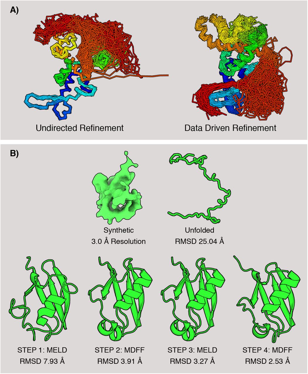
In data-rich situations, we first use MAINMAST to get a chain trace from the EM map. Then we use this starting model in an iterative cycle between ReMDFF simulations that keep secondary structures fixed, and MELD which explores a larger conformational space, including alternative secondary structures. Taken alone, ReMDFF fits models into electron density features, but fails to explore sufficient secondary structure17. MELD addresses this issue by partial folding, unfolding, and reformation of secondary structures18, 19. MELD is a method that can do full folding, starting only from a sequence, then using coarse physical information (CPI) – e.g. that proteins have hydrophobic cores, β-strand pairing and secondary structures consistent with a server19, 20 (Fig. 2A). Consequently, a hybrid iterative MELD-ReMDFF approach allows the determination of complete all-atom models starting only with sequence information and structural input data of varying coarseness. In data-poor situations, in principle, we do not require the MAINMAST first step. Nonetheless, backbone tracing accelerates convergence of CryoFold. We report 4 cryo-EM structure determination examples here, ranging from data-rich to data-poor, for proteins from 108 to 592 residues, and across both soluble and membrane proteins. CryoFold produces high-quality structures: it offers a high radius of convergence in the range of 50 Å refining soluble and transmembrane structures with consistently > 90% favored backbone and sidechain statistics, and high EMRinger scores. The results are independent of the initial estimated conformation and consistent with physics and stereochemistry. The method is automated and is available through a python-based graphical interface, with a video tutorial.

(A) Ensemble refinement with CryoFold showcased for the soluble domain of TRPV1. Several conformations from the TRPV1 ensemble are superimposed; color coding from blue (N-terminal) to red (C-terminal). In a MELD-only simulation, a soluble loop (indicated in red) artifactually interacted with the transmembrane domains. Following the data-guidance from ReMDFF, this loop interacted with the soluble domains and a more focused ensemble is derived that agrees with the electron density. (B) Stages of the refinement protocol for a test case, ubiquitin. The initial model is an unfolded coil. In two consecutive MELD-ReMDFF iterations the RMSD of the folded model relative to the crystal structure (1UBQ) attenuated from 25.04 Å to 2.53 Å.
Results
Ubiquitin with synthetic data
First, as a proof of principle, we used rich data on a small protein. From the known X-ray crystal structure of ubiquitin, we generated synthetic electron density at 3.0 Å resolution21, and asked if CryoFold could correctly recover the X-ray structure. In this rich-data situation, MELD was used to generate 50 search models from just the amino acid sequence, and no usage of the electron density data. Then, these models were rigid-fitted into the electron density using Chimera22, 23, and ranked based on their global cross-correlation. ReMDFF refined the best rigid-fitted model even further. The ReMDFF model with the highest Cross Correlation (CC) to the density map served as a template for the subsequent iteration with MELD. For ubiqui-tin, two such MELD-ReMDFF iterations (Fig. 2B) were sufficient to successfully predict a model having an RMSD difference of 2.53 Å from the X-ray crystal structure (PDB id: 1UBQ, see Table S1).
Ubiquitin at 3.0 Å resolution.
Tests on Flpp3, a membrane protein with a uniformly high-resolution structure
Flpp3 provides us with a validation test of CryoFold. It is a 108 amino acids long membrane protein that serves as a target for vaccine development against tularemia24. Electron density has already been obtained at 1.80 Å resolution by our Serial Femtosecond X-ray (SFX) crystallography experiments (See Supplementary Information). A key question for us was whether MELD could handle this size of protein, since MELD currently reaches only about 100 residues for ab initio folding, due to the combinatorics of the associated CPIs19. So here, we used MAINMAST16 to introduce the Cα traces as constraints for MELD (Fig. 3A). Convergent ensembles derived from this MAINMAST-guided MELD step were then refined by ReMDFF to improve the sidechains until the density was resolved with models of reliable geometry.
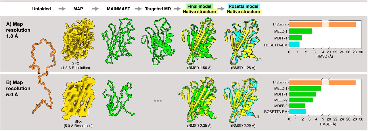
(A) High-resolution density map at 1.8 Å resolution. An unfolded structure was used as the initial model. A SFX density map at 1.8 Å resolution was employed to generate the Cα position (green spheres) using MAINMAST, and the initial model was fitted into these positions by targeted MD. The resulting structure (green cartoon model) was then subjected to MELD-ReMDFF refinement. This procedure yielded a structure with RMSD of 1.56 Å relative to the native SFX structure (yellow). The Rosetta-EM model (cyan) has an RMSD of 1.28 Å with respect to the SFX structure. (B) Lower-resolution density map at 5 Å resolution. An initial Cα trace in the map was computed using MAINMAST. Subsequent MELD-ReMDFF refinement resulted in a structure (green cartoon model) with an RMSD of 2.29Å from the SFX structure (yellow). The best Rosetta-EM model has (cyan) an RMSD of 2.35 Å to the SFX structure. Barplots depict the evolution of RMSD of the CryoFold models with each subsequent MELD-ReMDFF refinement.
We found that one iteration of the MELD-ReMDFF cycle sufficed to resolve an all-atom model of flpp3 from the SFX density with a global CC of 0.83 and Molprobity score of 0.93 (Table S2); RMSD of the CryoFold-derived model is 1.56 Å from the SFX model. The density data was truncated at 5 Å to examine the robustness of the refinement method at resolutions, where MAIN-MAST produced low quality backbone traces (Fig. 3B). Remarkably, even with low quality Cα traces, MELD-ReMDFF successfully produced models comparable to our high-resolution refinements. After two MELD-ReMDFF iterations, the best structure obtained was within 2.29 Å RMSD from the SFX model. The MELD-ReMDFF combination in CryoFold succeeds where other methods fail: While both the de novo Rosetta RASREC and MELD-only predictions modelled the β-sheets accurately, they failed to accurately converge on all helices (Fig. S1). For example, a 4-turn helix was underestimated to contain only 2-3 turns. The final CryoFold model had comparable geometry to that of the high resolution structure: 94.34 % Ramachandran favoured backbones and 98.78 % favoured sidechains and the reported molprobity score of 0.95 (Table S3).
Flippase at 1.8 Å resolution
Flippase at 5.0 Å resolution

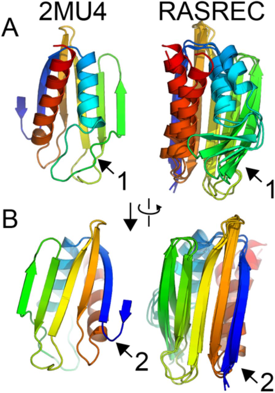
A) The structure of flpp3 show with rainbow coloring from the N-terminus (blue) to the C-terminus (red) and the superposed output from the top three clusters of the RASREC predictions. The data output shows that RASREC predicted the helices with relatively low convergence. Additionally, RASREC predicted β-sheets that were not observed in the SFX structure. B) A 90◦ rotation of the model illustrates that the β-sheets were predicted relatively well, but the N-terminal sheet was overestimated.
A comparison with Rosetta-EM generated structures suggests that the structures from the CryoFold were comparable in quality and accuracy for both the high and low resolution case. Rosetta-EM was able to generate structures, which were 1.28 Å for the 1.80 Å-map and 2.35 Å for the 5.00 Å-map. The best models obtained from the CryoFold protocol were at 1.56 and 2.29 Å respectively. Furthermore, the CryoFold model was comparable in geometry with the Rosetta-EM model for both 1.8 and 5.00 Å resolutions (Tables S2 and S3). This test shows that the CryoFold trio of methods gives accurate structures for longer chains than is otherwise possible with either one of these methods.
Tests in TRPV1, soluble domains of an integral-membrane protein with heterogeneous resolution
A major problem in cryo-EM structure determination is that the data is heterogeneous, offering models with highly resolved core conformations but poorly resolved peripheral regions. Examples are the cytoplasmic domains of the heat-sensing ion channel TRPV1 (592 amino acids long), where local-resolution of the experimental density varies between 3.8 to 6.0 Å 25, 26, as determined by Resmap27. Furthermore, TRPV1 has two apo-structures deposited in the RCSB database, one with moderately resolved transmembrane helices and cytoplasmic domains26 (pdb id:3J5P, EMDataBank: EMD-5778), and another with highly-resolved transmembrane helices (pdb id:5IRZ, EMDataBank: EMD-8118) but with the cytoplasmic regions, particularly the β-sheets, less resolved than in 3J5P. CryoFold was employed to regenerate these unresolved segments of the cytoplasmic domain from the heterogeneous lower-resolution data of 5IRZ. We compare the CryoFold model to the reported 3J5P structure (Fig. 4), where these domains are much better resolved showing clear patterns of β-strands. This case-study demonstrates how structures normally determined from high-resolution density data can now be extracted from data of much lower local-resolution using CryoFold.

(A) TRPV1 structures deposited in 2016 (pdb 5IRZ in yellow) and in 2013 (pdb 3J5P in cyan in cartoon representation, showing the latter has a more resolved β-sheet while the former possess an additional extended loop. (B) The 5IRZ model was heated at 600 K while constraining the α helices. This treatment resulted in a search model with the loop regions significantly deviated and the β sheets completely denatured. The search model was subjected to MELD-ReMDFF refinement. The final refined model agrees well with 5IRZ (C) Progress of the refinement in each step of CryoFold. MELD step 1 shows the β sheets modeled correctly, while the loops recovered in MDFF step 2, and refinement was complete by step 4.
A search model was created by heating the β strands of the cytoplasmic domain using brute force MD simulations at 600 K, keeping the rest of TRPV1 fixed. The strands transformed into a random polypeptide chain over 10 ns, yielding an unbiased starting point for the CryoFold refinements. A single round of MELD regenerated most of the β-sheet from this random chain, however the 5-to 15-residue long interconnecting loops still occupied non-native positions. Subsequent ReMDFF refinement with the 5IRZ density resurrected the loop positions. One more round of the MELD and ReMDFF resulted in the further refinement of the model. The final model was ob-served to be at an RMSD of 3.41 Å with a CC of 0.74 relative to 5IRZ. The same model with some loops removed for consistency with the EMD-5778 density produced an RMSD of 2.49 Å and CC of 0.73 with respect to 3J5P. Our approach resulted in a structure with 93.75% Ramachandran favored backbones and 92.37% favored sidechains and the Molprobity score of 1.67 (Table S4). In comparison, the deposited high-resolution structure (5IRZ) had 92.64% Ramachandran favored backbones and 98.90% favored sidechains, and a Molprobity score of 1.99. Furthermore, the EM-ringer score of our model was observed to be 3.35 with respect to the 5IRZ density; the same for the original model was 3.26. A model derived from our Rosetta enumerative sampling (Rosetta-ES) refinement28 of the 5IRZ density had a Molprobity score of 3.56 with 73.02% Ramachandran favored backbones. Furthermore, the Rosetta-ES model showed a clash score of 7.92, owing to an unphysical overlap between the β-sheet and the loop (Fig. S2), making the sidechain-geometries unreliable.
TRPV1 soluble domain

(A) Comparison between the Rosetta-EM model (cyan cartoon) and the native structure (red transparent) of the cytoplasmic domain of TRPV1. Arrows denote erroneous modeling of the loop on the top of β sheets in the Rosetta-EM model. (B) Comparing the CryoFold model (grey cartoon) and the native structure (red transparent cartoon). Note that the CryoFold model agrees well in both the loop and the β-sheet region with the native model.
Interestingly, as part of the 2016 Cryo-EM modeling challenge, TRPV1 benefits from the submission of 22 structures into the competition database for 3J5P. Presented in Table S5, our TRPV1 model (model no. 4), with a loop removed to be consistent with 3J5P, represents the higher end of the CC-scores, and the top quarter of the entries with > 90% Ramachandran favored statistics. The EMRinger score of 2.54 with respect to 3J5P is an improvement from our previous submission of 2.25 to the competition (and originally reported value of 1.75), also featuring the top - 20% of the submissions. This improvement is attributed solely to the higher-quality β-sheet models that is now derived from simultaneously running MELD and ReMDFF. Surprisingly, CryoFold allows determination of models commensurate to the 3J5P density starting with 5IRZ, where the β-sheets were originally less resolved - an outcome of enhanced sampling and first-principles physics that is integrated by the method. Taken together, models derived from the CryoFold refinement of 5IRZ capture in atomistic details the highly resolved features of this density, yet without compromising with the mid-resolution cytoplasmic areas where it performs as well as the 3J5P model.
TRPV1 deposited models
Tests in CorA, soluble and TM domains of a large ion channel at mid resolution
One of the grand challenges in de novo structure determination arises from the modeling of complete trans-membrane protein systems, including structure of both the soluble and TM domains. Addressing this challenge, CryoFold was employed to model a monomer from the pentameric Magnesium channel CorA, containing 349 residues, at 3.80 Å resolution29 (pdb id: 3JCF, EMDataBank: EMD-6551) (Fig. 5). An initial topological prediction of the channel was obtained by flexibly fitting of a linear polypeptide onto the Cα trace obtained from the cryo-EM density using MAINMAST. Leveraging the resulting structure, MELD was used to perform local conformational sampling, regenerating most of the secondary structures. The model with the highest cross-correlation to the map was then refined using ReMDFF, finally resulting in models which were at 2.90 Å RMSD to the native state. Even though this model possessed high secondary structure content 76%, sub-stantial unstructured regions remained both in the cytoplasmic and the transmembrane regions, warranting a further round of refinement. In the subsequent MELD-ReMDFF iteration, the re-sulting models were 2.60 Å to the native state and agreed well with the map with a CC of 0.84. Moreover, the CryoFold models were comparable in geometry to that deposited in the database. Presented in Table S6, the Molprobity score of the CryoFold model (0.94) is a clear improvement over that of the deposited model (1.75). A model obtained from Rosetta-EM was comparable in geometry to both the CryoFold and the deposited model Table S6. However, the Rosetta-EM model was at 4.20 Å RMSD to the native state, in comparison the CryoFold model was at 2.60 Å (Fig. 5A,D). Closer inspection of the models reveal that the Rosetta-EM did an excellent job at modeling the α helices, but it models the β-sheets in the cytoplasmic domain as unstructured (Fig. 5D). In comparison the CryoFold provided credible models for both the α helix and the β sheet regions.
Mg 2+ Channel CorA at 3.8 Å resolution

The CryoFold protocol on CorA. A Cα trace (green spheres) was generated from the Cryo-EM density map (EMD-6551) using MAINMAST. A random coil (orange) was fitted to this map using targeted MD to generate initial search model (green cartoon). Two concurrent rounds of MELD-ReMDFF refinement generated a structure that agrees extremely well with the native structure (yellow). The resultant CryoFold model is at an RMSD of 2.60 Å relative to the native structure and features accurate beta structures. (B) Ensemble of models at MELD refinement stage step1 and step 2. Ensemble models of step3 is showing convergence after three iterations. (C) The evolution of the RMSD of CryoFold models with each MELD-ReMDFF refinement. (D) The Rosetta-EM model (cyan) and the native structure (yellow). This model is at an RMSD of 4.20 Å with respect to the native structure.
While CryoFold appears promising for obtaining biomolecular structures from cryo-EM, we are aware of some limitations. First, its success depends upon the correctness of the initial trace generated by MAINMAST. It is not clear when and whether the MD tools can recover from a wrong chain trace. Second, as with any MD simulation of biomolecules, the force fields are still not perfect and larger structures will be a challenge for the searching and sampling, even with an accelerator such as MELD.
Conclusions
Over the past half century, structural biology has been powered by data-rich methods such as X-ray crystallography and solution NMR, combined with computations such as XPLOR-NIH, PHENIX and molecular dynamics simulations. The Protein DataBank has more than 150,000 structures at around 2 Å resolution. Cryo-EM is a powerful new method for molecules in large complexes, in membranes, or that do not crystallize, but it is data poor, giving information only to around 3-5 Å resolution. Cryo-EM poses a much more demanding challenge for computational algorithms that convert density maps into molecular structures. While there have been some successes in ab-initio model-building (Fig. S3)10, 30, there is a major need for better computer methods; namely, that are automated and can handle limited data, large complexes and heterogeneous resolution.

Here, we describe a computational method called CryoFold, which combines the MAIN-MAST ability to determine a chain trace from EM data, with the ReMDFF Molecular Dynamics simulation engine, accelerated by MELD to refold and sample the larger conformational spaces that can improve secondary and tertiary structures. We describe here 4 successful examples, including membrane proteins, indicating that CryoFold is a useful computational tool for obtaining molecular structures from cryo-EM data.
Methods
The data-guided fold and fitting paradigm presented herein combines three real-space refinement methodologies, namely MELD, MAINMAST and ReMDFF. In what follows, these three formula-tions are articulated individually. Hybridization of the methods gives rise to a molecular dynamics-based de novo structure determination tool, CryoFold. The general principles of ensemble refinement within CryoFold are described. Details of the computational implementation, including a description of the GUI, are relegated to the Supplementary Information.
MELD
Modeling Employing Limited Data (MELD) employs a Bayesian inference approach (eq. (1)) to incorporate empirical data into MD simulations18, 19. The bayesian prior  comes from an atomistic force field (ff14SB sidechain, ff99SB backbone) and an implicit solvent model (Generalized born with neck correction, gb-neck2) 31, 32. The likelihood
  representing a bias towards known information, determines how well do the sampled conformations agree with known data,
  refers to the likelihood of the data, which we take as a normalization term that can typically be ignored. Taken together,
 The kind of data that MELD is designed to handle has one or more of the following features: sparsity, noise and ambiguity. Brute-force use of such data is deemed inadequate for complete structure determination30. A typical MD simulation starts from accurate initial models derived with high-resolution structural data. However, at low resolutions assessing the quality of experimental data is ambiguous, often resulting in the determination of incorrect models. MELD addresses the refinement of low-resolution data by enforcing only a fraction (x%) of this data at every step of the MD simulation. Although x is kept fixed, the subset of data chosen to bias the simulation keeps changing with the simulation steps. This data is incorporated as flat-bottom harmonic restraints E(rij) for evaluating the likelihood
  .
.
 When these restraints are satisfied they do not contribute to the energy or forces, contributing for flat bottom region of eq. 2 and (Fig. S4). When the restraints are not satisfied they add energy penalties and force biases to the system – guiding it to regions that satisfy a subset of the data, or conformational envelopes. Details of MELD implementation are provided in Supplementary methods: Description of MELD.

MELD tries to satisfy subsets of noisy data, effectively creating conformational envelopes where there is no bias and other regions that funnel structures towards the closest envelope. A hamiltonian and temperature replica exchange ladder is used where the data is not enforced at the highest replica (where the temperature is also high) and are strongly enforced at the lowest replica ladder.
MAINMAST
MAINchain Model trAcing from Spanning Tree (MAINMAST) is a de novo modeling program that directly builds protein main-chain structures from an EM map of around 4-5 Å or better resolutions16. MAINMAST automatically recognized main-chain positions in a map as dense regions and does not use any known structures or structural fragments.The procedure of MAINMAST consists of mainly four steps (Fig. S5). In the first step, MAINMAST identifies local dense points (LDPs) in an EM map by mean shifting algorithm. All grid points in the map are iteratively shifted by a gaussian kernel function and then merged to the clusters. The representative points in the clusters are called LDPs. In the second step, all the LDPs are connected by constructing a minimum spanning tree (MST). It is found that the most edges in the MST covers the main-chain of the protein structure in EM map16. In the third step, the initial tree structure (MST) is refined iteratively by the so-called tabu search algorithm. This algorithm attempts to explore a large search space by using a list of moves that are recently considered and then forbidden. In the final step, the longest path of the refined tree is aligned with the amino acid sequence of the target protein. This process assigns optimal Cα positions of the target protein on the path and evaluates the fit of the amino acid sequence to the longest path in a tree. Details of MAINMAST implementation are provided in Supplementary methods: Description of MAINMAST.

Four steps of MAINMAST algorithm are illustrated with example for flpp3. First, local dense points are identified with the mean shift algorithm. Identified local dense points are connected by minimum spanning tree (MST) (cyan). Using tabu-search, the MST is refined, iteratively. The amino acid sequence of the query protein is mapped on the longest path in the tree. Cα models from each generated longest path are ranked with the density–volume matching (threading) score. In the first panel on the right, the local dense points are colored by the scale of density, blue to orange for low to high density. The second panel shows the minimum spanning tree. In the third panel, the chain represents a predicted Cα model.
Traditional MDFF
The protocol for molecular dynamics flexible fitting (MDFF) has been described in detail7. Briefly, a potential map VEM is generated from the cryo-EM density map, given by
 where Φ(r) is the biasing potential of the EM map at a point r, ζ is a scaling factor that controls the strength of the coupling of atoms to the MDFF potential, Φthr is a threshold for disregarding noise, and Φmax = max(Φ(r)).
A search model is refined employing MD, where the traditional potential energy surface is modified by VEM. The density-weighted MD potential conforms the model to the EM map, while simultaneously following constraints from the traditional force fields. The output structure offers a real-space solution, resolving the density with atomistically detailed structures.
ReMDFF
While traditional MDFF works well with low-resolution density maps, recent high-resolution EM maps have proven to be more challenging. This is because high-resolution maps run the risk of trapping the search model in a local minimum of the density features. To overcome this unphysical entrapment, resolution exchange MDFF (ReMDFF) employs a series of MD simulations. Starting with i = 1, the ith map in the series is obtained by applying a Gaussian blur of width σi to the original density map. Each successive map in the sequence i = 1, 2, . . . L has a lower σi (higher resolution), where L is the total number of maps in the series (σL = 0 Å). The fitting protocol assumes a replica-exchange approach described in details17 and illustrated in Fig. S6. At regular simulation intervals, replicas i and j, of coordinates xi and xj and fitting maps of blur widths σi and σj, are compared energetically and exchanged with Metropolis acceptance probability
 where kB is the Boltzmann constant, U (x, σ) is the instantaneous total energy of the configuration x within a fitting potential map of blur width σ. Thus, ReMDFF fits the search model to an initially large and ergodic conformational space that is shrinking over the course of the simulation towards the highly corrugated space described by the original MDFF potential map. Details of ReMDFF implementation are provided in Supplementary methods: Description of Resolution exchange MDFF.

Three replicas are included in this schematic. Each replica consists of a molecular structure and a cryo-EM map-based grid potential. Different green boxes represents grid potentials of different resolutions. The structural models as refined at different resolutions are shown in red, orange, and yellow with different hue levels representing changes in the conformation. The arrows indicate the transfer of a grid potential from one replica to another. The output structure is selected from the trajectory visited by the grid potential of the original resolution (dark green).
CryoFold (MELD-MAINMAST-ReMDFF) protocol
Illustrated in Fig. 1, the CryoFold protocol begins with MELD computations, which guided by backbone traces from MAINMAST yields folded models. These models are flexibly fitted into the EM density by ReMDFF to generate refined atomistic structures.
First, information for the construction of Bayesian likelihood is derived from secondary structure predictions (PSIPRED), which were enforced with a 70% confidence. This percentage of confidence offers an optimal condition for MELD to recover from the uncertainties in secondary structure predictions20. For membrane proteins, this number can be increased to 80% when the transmembrane motifs are well-defined helices. MELD extracts additional prior information from the MD force field and the implicit solvent model (see eq.1).
In the second step, any region determined with high accuracy will be kept in place with cartesian restraints imposed on the Cα during the MELD simulations. This way, the already resolved residues can fluctuate about their initial position.
In the third step, distance restraints (e.g. from the Cα traces of MAINMAST) are derived. The application of MAINMAST allows construction of pairwise interactions as MELD-restraints directly from the EM density features. Together with the cartesian restraints of step 2, these MAINMAST-guided distance restraints are enforced via flat-bottom harmonic potentials (see eq. 2) to guide the sampling of a search model; notably, the search model is either a random coil or manifests some topological features when created by fitting the coil to the Cα trace with targeted MD. Depending upon the stage of CryoFold refinements, only a percent of the cartesian and distance restraints need be satisfied. The cartesian restraints are often localized on the structured regions, while the distance restraints typically involve regions that are more uncertain (e.g loop residues).
Fourth, a Temperature and Hamiltonian replica exchange protocol (H,T-REMD) is employed to accelerate the sampling of low-energy conformations in MELD18, 19, refining the secondary-structure content of the model. The Hamiltonian is changed by changing the force constant applied to the restraints. Simulations at higher replica indexes have higher temperatures and lower (vanishing) force constants so sampling is improved. At low replica index, temperatures are low and the force constants are enforced at their maximum value (but only a certain per cent of the restraints, the ones with lower energy, are enforced). See SI for details for individual applications.
Fifth, cross-correlation of the H,T-REMD-generated structures with the EM-density is employed as a metric to select the best model for subsequent refinement by ReMDFF (Fig. S7). Resolution exchange across 5 to 11 maps with successively increasing Gaussian blur of 0.5 Å (σ in eq. 4) sufficed to improve the cross-correlation and structural statistics. The model with the highest EMringer score forms the starting point of the next round of MELD simulations. Thereafter, another round ReMDFF is initiated, and this iterative MELD-ReMDFF protocol continues until the δ CC between two consecutive iterations is <0.1.

Cross correlation score vs (A) trajectory length or (B) rmsd to native. The cross correlation score increases through simulation time and is a good indicator of protein quality when compared to rmsd (Å). Colors indicate two starting structures: the blue dots correspond to a trajectory that comes from a low resolution backbone tracing and the orange ones from a high resolution backbone trace.
Throughout different rounds of iterative refinement, the structures from ReMDFF are used as seeds in new MELD simulations. At the same time, distance restraints from the ReMDFF model are updated and the pairs of residues present in those interactions are enforced at different accuracy levels.
As expected, the more rounds of refinement we do, the higher the accuracy levels for the contacts is achieved in CryoFold. In going through this procedure, the ensembles produced get progressively narrower as we increase the amount of restraints enforced.
Competing Interests
The authors declare that they have no competing financial interests.
Supplementary Methods
Description of MELD
Modeling Employing Limited Data (MELD) employs a Bayesian inference approach (eq. (1)) to incorporate empirical data into MD simulations1, 2. The prior  comes from an atomistic force field (ff14SB sidechain, ff99SB backbone) and an implicit solvent model (Generalized born with neck correction, gb-neck2) 3, 4. The likelihood
  determines how well do the sampled conformations agree with known data.
  refers to the likelihood of the data, which we take as a normalization term that can typically be ignored.
 The kind of data that MELD is designed to handle has one or more of the following features: sparsity, noise and ambiguity. Brute-force use of such data is deemed inadequate for complete structure determination. A typical MD simulation starts from accurate initial models derived with high-resolution structural data5. However, at low resolutions assessing the quality of experimental data is ambiguous, often resulting in the determination of incorrect models. MELD addresses the refinement of low-resolution data by enforcing only a fraction (f%) of this data at every step of the MD simulation. Although the fraction (f) is kept constant during the simulation, the feature of the data used at every step is determined on the flight. For each data point we calculate a penalty term based on flat-bottom harmonic restraints (see eq. 2) which serves as the way of evaluating the likelihood
 When these restraints are satisfied they do not contribute to the energy or forces (flat bottom region see eq. 2 and Fig. S3). When the restraints are not satisfied they add energy penalties and the resulting force biases to the system, guiding it to regions that satisfy a subset of the data, or conformational envelopes.
For every structure, the energy restraints are evaluated for all the data provided. These restraints are sorted according to their magnitude, and only those in the lowest f% are chosen to guide the simulation until the next step. Consequently, the forces and energies acting on the system are deterministic: given a structure, the force field terms (priors in eq. 1) are computed, and the biasing forces are added as the subset of restraints that yield the lowest energy for the structure being sampled1. A Temperature and Hamiltonian replica exchange molecular dynamics protocol (H,T-REMD) is employed to accelerate the sampling of these low-energy conformations. The Hamiltonian changes by effectively changing the strength of the force constant used for the restraints (product w(λ)k, where k is the force constant of the restraint and w(λ) is the weight assigned to a particular replica (see eq. 2). The parameter λ is used to map replica numbers to a value between 0 (lowest replica) and 1 (highest replica).
At the lowest replica index we sample from room temperature (300K) and we enforce the flat-bottom harmonic restraints at their maximum (w(λ)=1). At the highest replica index, the temperature is at its maximum (450K) and w(λ)=0 (we sample freely over the energy landscape). We used 30 replicas in all cases, and scaled the Hamiltonian and temperature ladders following previous protocols2.
The resulting MELD ensembles are processed by analyzing the lowest temperature replicas, which represent the flat region of the energy restraints (the energy will be the same as in the original force field). A standard 2D-RMSD clustering protocol (Fig. S6) for structural similarity6 is used to identify the lowest free energy structures.
Description of MAINMAST
MAINMAST (MAINchin Model trAcing from Spanning Tree) is a de novo modeling program that directly builds protein main-chain structures from an EM map of around 4-5 Å or better resolutions7. MAINMAST automatically recognized main-chain posi-tions in a map as dense regions and does not use any known structures or structural fragments.The procedure of MAINMAST consists of mainly four steps (Fig. S5). In the first step, MAINMAST identifies local dense points (LDPs) in an EM map by mean shifting algorithm. The mean shifting algorithm is a non-parametric clustering algorithm that was originally developed for image processing. In the MAINMAST algorithm, the assumption is that a density observed in an EM map is the sum of Gaussian density functions that originate from atom positions and the local maxima of dense regions corresponds to the atomic positions of the protein structure. All grid points in the map were iteratively shifted by a gaussian kernel function and then merged to the clusters. The representative points in the clusters are called LDPs. In the second step, all LDPs are connected by constructing a minimum spanning tree (MST). MST is a graph structure that connect all nodes with the minimal total weight of edges by a three-graph structure (i.e. no-cycle graph). We used the Euclidean distance between the two nodes as the weight of the edge. It was found that the most edges in the MST covers the main-chain of the protein structure in EM map. In the third step, the initial tree structure (MST) is refined iteratively by tabu search algorithm8. The longest path in the MST usually contains some wrong connection and disconnections. Therefore, the longest path in the MST cannot complete whole main-chain structure. In order to refine the MST, MAINMAST performs a tabu search method. A tabu search attempts to explore a large search space by using a list of moves that were recently considered and then forbidden. In the final step, the longest path of the refined tree is aligned with the amino acid sequence of the target protein. This process assigns optimal Cα positions of the target protein on the path and evaluates the fit of the amino acid sequence to the longest path in a tree. For example, amino acids with a large side-chain are mapped to a position on the path with a high density and large volume. All the steps are performed multiple times with various parameter combinations, and then over six thousand Cα models were generated. The models are then ranked with the density-volume matching (threading) score. For flpp3 and TRPV1, MAINMAST generated 6,048 and 8,065 Cα models, respectively.
Description of Resolution exchange MDFF
Main computational steps involved in an ReMDFF refinement9 is described as follows (Fig. S4): First, the reported map is smoothed employing Gaussian blurs with the half width σi uniformly spaced at 0.5 Å. As a result a set of at most 11 density maps with varied local resolution were generated. Second, the initial model obtained from the MELD simulation is docked in the EM density using e.g., Situs 10 or Chimera11, 12. The map with the lowest resolution was chosen for this purpose. Third in order to prevent over-fitting to the density, chirality and cis-peptide restraints are generated from the initial model according to protocols defined in (Schreiner et al., 2011). Finally in accordance to the scheme shown in (Fig. S4), the resolution exchange program is invoked within NAMD, performing ReMDFF. The map-model coupling parameter is empirically determined and is generally set between 0.3-0.6. In the replica-exchange scheme, exchanges were attempted every 20,000 steps. Depending on the system, exchange rates of 30%–60 % was achieved. Simulations were performed in implicit solvent environment using CHARMM36m protein force field.
Supplementary Notes
CryoFold for Ubiquitin
The synthetic density for ubiquitin was constructed using phenix.maps with the diffraction data reported for PDB:1UBQ, truncated at 3 Å. A standard MELD-CPI run was performed with 30 replicas1, 13 starting from an extended state and simulated for 25 ns. 50 evenly spaced structures were collected from the highest and lowest temperature replica. Typically, at least 500 ns sampling is required to get native-like topologies for ubiquitin13. To avoid this prohibitively long MD simulation, MAINMAST and a synthetic density map for ubiquitin were used to generate a series of alpha carbon traces ranging in quality. A conformation with high RMSD to the native structure (since it is known) was chosen from the MELD ensemble (25th frame in this case). Targeted MD was performed for 10 ns with this conformation and the target-RMSD delivered from the Cα tacting as restraints. This targeted MD run improved the ubiquitin structure dramatically.
At this point a second MELD run was set up wherein, Cα contacts below 6Å and separated by more than four residues in the chain were calculated. Analogous to previous structure modeling using MELD1, 13, these contacts were enforced in a MELD run starting from the given structures at 60% accuracy. Simulations were run for Cα 100 ns with this data and secondary structure predictions (PSIPRED) enforced. From these trajectories we selected frames based on the best cross-correlation overlap, which were fed to the MDFF machinery. Cross-correlation improved with trajectory length and correlated well with RMSD (see Fig. S7).
After these structures were further improved with ReMDFF, three new simulations were started in MELD, from different accuracies in MDFF (3, 4 and 5 Å). The same MELD protocol as in step 2 (Fig. 3) was used. In all cases, running microsecond long simulations resulted in frames of accuracy better than 2.5 Å. Selection of good models can be achieved either on the basis of clustering or by selecting on the basis of higher cross-correlation. These structures are then reintroduced into ReMDFF for a last stage of refinement. Altogether, the combination of MELD and ReMDFF defines new secondary structure elements and orientations and packing them to high accuracy within the density map.
CryoFold for flpp3
CryoFold was utilized to generate ensembles of flpp3 structures from maps of resolution varying between 1.8 –5 Å. The serial femtosecond crystallography data used for these computations and the high-resolution flpp3 structure determined using traditional methods used here for benchmarking CryoFold are published independently. The companion manuscript is provided for now as additional supporting information.
Starting from a high resolution map of 1.8 Å, a low resolution map of 5 Å was generated by truncating the diffraction data with phenix.maps. Thereafter, initial protein topology to be used in MELD as pairwise distance restraints was obtained by generating Cα traces using MAINMAST for both the 1.8 Å and the 5 Å maps. At 5 Å the tracing of the Cα by MAINMAST was significantly worse than the other cases, with atoms overlapping (Fig.3A,B). Hence, the 5Å resolution was used as representative of a low resolution (data-poor) refinement.
MAINMAST structures were used to construct a contact map between Cα atoms, consid-ering all contacts with distances beneath 8 Å and separated by at least 4 residues in the linear chain. These contacts were enforced at 80% accuracy inside MELD simulations – these simulations started from an extended chain as prepared by AMBER’s tleap program. At any stage in which MELD structures were refined with MDFF, we used these model as both an initial point and to calculate a contact map. We selected distances below 6 Å from the contact map and enforced them at 60%. This guarantees that we sample structures that are close to the MDFF model, but with enough wiggle room for refinement.
At the low resolution of 5 Å there was a higher level of uncertainty in the positions of the Cα atoms resulting in a concomitant inaccuracy of the predicted distances between these atoms. We used the mainmast structure to calculate a contact map, from which we selected non sequence-local contacts that were beneath 8 Å. Due to the aforementioned higher levels of uncertainty in Cα positions, restraints were enforced in three different protocols namely (1) 8 Å (15% accuracy), (2) 9 Å (20% accuracy) or (3) 10 Å (25% accuracy). At the end of these simulations the best structures from the trajectories (at least 750 ns long) were selected via cross correlation with the 5 Å map. The protocol with 20% of contacts enforced at 9 Å performed the best and hence its structures were used for ReMDFF refinement. Structures from ReMDFF were then used for another stage of MELD refinement. We know that at each round the accuracy gets better, but we do not know how much. Hence we tried five simultaneous protocols in which the ReMDFF structures were used as starting models and the contacts between Cα atoms were enforced at 8 Å with an accuracy of either 55, 65, 75, 85 or 95%. The cross correlation was used to select the best protocol to carry forward. For MELD, care needs to be taken to not enforce more data than is present in the native state.
Otherwise, one runs the risk of obtaining a non-native lowest free energy state. The accuracy is usually known for a given set of data (e.g. NMR, EPR, …). However, for cryoEM, the diversity of tools and resolutions make it hard to come up with a general strategy. At the same time, the density map provides a perfect way to score structure in the ensemble. Hence, several different strategies covering a wide range of conditions can be started simultaneously with MELD and the ones providing the best agreement with the experimental data can be carried forward. This gives the user plenty of flexibility and, with enough resources, the simulations will all occur in the same amount of time (all the results of the current work was obtained within a week using Blue Waters supercomputer – pharma companies with enough cloud resources could access as many simultaneous simulations as they wanted. A GUI is provided to generate inputs for MELD).
CryoFold for TRPV1
TRPV1 presents a unique case to test capabilities of CryoFold on systems with heterogeneous CryoEM densities. Concentrating on only the soluble domain of TRPV1, the protein was truncated at its membrane interface, while also fixing the interfacial residues with cartesian restrains. This approach enables the application of our methodology to large macro-molecules by fragmenting it into several independent smaller domains. Of particular interest in the soluble domain are β-sheets and a loop (residues 112-122 and 184 to 224) connecting the sheets to the transmembrane domain. These structural elements were heated at 450 K for 10 ns converting them to an unstructured polypeptide chain. Beginning the CryoFold refinement, in the MELD setup 40% of the PSIPRED-predicted secondary structures were enforced for these two regions. A list of all possible contacts between the aforementioned region of interest and additional packing areas within a radius of 8Å (residues 19 to 52 and 81 to 94) was created. At each MELD timestep at most 10 of the total 1610 possible contacts were enforced. This folding procedure resulted in an ensemble of conformations, where the β-sheets were packed close to the desired density, while loop occupies non-native regions. In order to filter a structure from the ensemble, cross-correlation to the map was calculated. Structure which had the highest cross-correlation serves as the most representative structure i.e, closet to the density among the MELD ensemble. Subsequently, ReMDFF refinement was initiated from this representative structure using 11 maps of resolution blurred in-crementally by steps of 0.5 Å Gaussian half-width. ReMDFF was able to improve on the loop conformation and the structure with the best cross-correlation was fed in the next round on MELD simulations. In a subsequent round, the contacts present in ReMDFF’s structure affecting the region 189-224 were identified resulting in 39 contacts. MELD was asked to satisfy 10, 20 or 30 contacts in three different simulations (each with 30 replicas). Cross-correlation score of the ensemble of MELD structures was used to determine the best structures to feed into a final round of ReMDFF refinement.
CryoFold for CorA
Pentameric Magnesium channel CorA serves as another transmembrane protein (resolved at 3.8 Å) system that was attempted for modeling. Initial position of the Cα atoms were generated using MAINMAST. Thereafter, targeted MD simulation was initiated to fit a linear polypeptide to the MAINMAST-generated Cα positions. The structure obtained served as a template for MELD simulations. Given the high confidence on the Cα positions for the amino acids and the lack of a good membrane implicit solvent, cartesian restraints were used on all Cα positions. Secondary structure prediction was imposed at 80% since membrane protein structure predictions were more accurate than the globular ones. MELD structures recovered a large fraction of secondary structure but introduced small kinks and discontinuities in some places of the transmembrane helix. Structure with high cross-correlation to the cryoEM densities was chosen to be refined by ReMDFF. ReMDFF was initiated using 11 densities with highest resolution density to be the experimentally determined one at 3.8 Å, the resolution blurred by Gaussian smoothing in steps of 0.5 Å. Thereafter, the structure with the highest cross-correlation to the map with highest resolution served as the template for another round of MELD simulations. Thereafter one more round of ReMDFF refinement was initiated from the best structure i.e., the one with cross-correlation to the map.
ROSETTA comparison
Rosetta de novo modeling for flpp3
The flpp3 secondary structure was predicted with Jufo9d14 and PSIPRED15, 16 servers. Nine- and three-mer fragments were generated using weighted quota protocols such that the PSIPRED and Jufo9d secondary structure predictions contributed to the fragment secondary structures equally. To eliminate bias for benchmarking purposes, the PDB 2MU4, corresponding to the structure of flpp317 was omitted during the fragment generation stage. The DUF3568 Family Protein from Francisella tularensis virulence determinant sequence (Uniprot: Q5NF33) was used as input for the fragment generation. As per standard prediction protocols, 1000 peptide candidates were considered with the top scoring 200 used as the final fragments for the de novo fold.
After generating fragments, de novo structure prediction was employed using the automated Rosetta protocol resolution-adapted recombination of structural features (RASREC)18. Extensive RASREC details are available in the original publication, however control of model generation can be altered in several ways. For this study, RASREC generated decoys were calculated using default flags, which automates decoy selection through four stages of centroid model generation and two stages of full atom decoy relaxation until convergence is achieved. RASREC has been successfully used in previous studies using sparse NMR restraints and co-evolved position contacts as restraints to generate de novo models; however, structural restraints nor evolutionary information were not employed for this study and the de novo folds relied solely on fragment inputs.
The RASREC algorithm is written to accept or discard until the pool size is full of decoys that were selected by the work-load manager. The end of the run generates a final pool of decoys, which contain as many decoys as specified by the pool size flag. With flpp3, this pool size was set to 500 decoys, which is the default setting. We clustered these 500 decoys using Calibur with default settings and then analyzed the RMSD of these clusters in PyMol by aligning the Cα atoms of β-sheets (residues 6-8, 11-18, 47-51, 55-61, 69-77, 93-112) and α-helices (residues 20-33, 93-112). The flpp3 de novo folding prediction was carried out with only fragments for inputs and achieved converged folds that are similar the NMR determined structure (Fig S1). Relying solely on fragments derived from secondary structure predictions Rosetta predicted flpp3 to an RMSD of 2.3 Å 3.3 Å and 1.8 Å of the 1st, 2nd, and 3rd largest cluster representatives, which was the lowest scoring decoy from each cluster. In Fig S1A, 2MU4 is shown for state 1 of the NMR ensemble next to the superposed decoys from decoys from the clusters. The α-helices do not appear to reach convergence, and RASREC predicted a β-sheet after the first α-helix (arrow #1). Fig S1B, shows that the β-sheets were predicted very well; however, the β-sheet N-terminal fold is missing in the RASREC predicted decoys (arrow #2).
Rosetta-ES de novo loop modeling for TRPV1
Rosetta ver. 3.9 (rosetta bin linux 2018.33.60351 bundle) was used. We followed the tutorial released on the tutorial website 19. All the parameters used were as described in the tutorial. First, nine and three residue fragment structures for the query protein were generated by grower prep in the Rosetta package. Then, the RunRosettaES.py script 20 built each segment from the generated fragments. The rebuilt regions were assembled by a Monte Carlo Assembly algorithm in the RunRosettaES.py. After the assembly step, the total 100 models were generated and ranked by Rosetta Energy. It should be noted that all generated models have steric clashes. Therefore, we could not have performed further Rosetta refinement.
Rosetta-EM de novo modeling for flpp3 and CorA
First, nine residue fragment structures for the query protein were generated on the Robetta website (http://robetta.bakerlab.org/fragmentqueue.jsp). We excluded fragments from homologues proteins. We performed a local fragment search in an in-put EM map by using denovo density. This procedure searches the density map for each sequence-predicted backbone fragment generated in the previous step. In the denovo density command, the number of translations to search (option: -n_to_search) was set to two times the number of residues. The number of intermediate solutions to keep (option: -n_filtered) was set to ten times the number of residues. The placed fragments were assembled by Monte Carlo sampling, then the consensus was assigned from the Monte Carlo trajectories. The final output file of the consensus assignment was used as input to RosettaCM. RosettaCM was applied to fill gaps where the fragments were not assigned by denovo density to complete a model and to refine the overall model structure. A total of 1,100 full-atom models were generated by RosettaCM. All of the 1,100 full-atom models were ranked by the total score (Rosetta Energy + density score). We selected the best 10% of the ranked models, and then selected the best model based on the density score.
Graphical User Interface
Requirements
MAINMAST requires 40-200 CPU hrs for the full-automated computation. This time could be reduced if the user manually checks the models of backbone trace by eye.
MELD requires 30 dedicated GPUs and a couple of days depending on the system size. MELD currently performs synchronous REMD, so each GPU is a different replica.
ReMDFF requires 1-2 days on 11 CPUs, depending on system size.
Note that the CryoFold GUI currently supports MDFF, not ReMDFF. MDFF requires less CPU-hours than ReMDFF.
Installation
The CryoFold GUI is optimized for LINUX/macOS distributions.
Anaconda and GFortran needs to be installed on your workstation in order to run the CryoFold GUI. CryoFold has four sections, namely, MAINMAST, TMD, MDFF and MELD. The GUI submits MAINMAST and MELD jobs, which requires these softwares to be installed as well. For TMD and MDFF, CryoFold GUI generates NAMD input scripts that the user can submit manually (NAMD need not be installed to run the GUI). However, these two sections require VMD to be installed.
- Anaconda installation: https://www.anaconda.com/distribution/
- GFortran installation: https://gcc.gnu.org/wiki/GFortran
- VMD installation: https://www.ks.uiuc.edu/Research/vmd/
- NAMD installation (not required to run GUI): https://www.ks.uiuc.edu/Research/namd/
- OpenMM installation: https://github.com/pandegroup/openmm
- MELD installation: https://github.com/maccallumlab/meld
Linux installation
After downloading and unzipping the folder, open a terminal and go to the CryoFoldGUI folder. Run install_linux.sh script to install everything needed - GFortran compilation of Mainmast and ThreadCA, Anaconda environment creation, python packages (kivy, numpy, mdtraj and meld). Finally, run start.sh to launch the CryoFold GUI.
MacOSX installation
After downloading and unzipping the folder, open a terminal and go to the CryoFoldGUI folder. Run install_mac.sh script to install everything needed - GFortran compilation of Mainmast and ThreadCA, Anaconda environment creation, python packages (kivy, numpy, mdtraj and meld). Finally, run start.sh to launch the CryoFold GUI.
Manual installation
Alternatively, the packages could be installed manually with the instructions on the following page:
- Numpy: https://anaconda.org/anaconda/numpy
- Mdtraj: https://anaconda.org/omnia/mdtraj
For gfortran compilation of MAINMAST and ThreadCA, run the following commands from the command line:
gfortran ./MAINMAST GUI/MainmastThreadCA/MAINMAST.f -w -O3 -fbounds-check -o ./MAINMAST GUI/MainmastThreadCA/MAINMAST -mcmodel=medium
gfortran ./MAINMAST GUI/MainmastThreadCA/ThreadCA.f -w -O3 -fbounds-check -o ./MAINMAST GUI/MainmastThreadCA/ThreadCA -mcmodel=medium
The CryoFold GUI can then be launched by running gui.py by typing “python gui.py” or by creating an executable.
Notes
Manual changes to installation script (install linux.sh or install mac.sh) might be necessary. Line 10 of the script specifies python version 3.5, which the user can change as per their choice. Additionally, MELD is available for CUDA versions 7.5, 8.0, 9.0 and 9.2. The current script will install meld-cuda75 (line 10), which is for CUDA 7.5. The user can manually change this (to meld-cuda80, meld-cuda90 or meld-cuda92) to suit their CUDA compiler.
We recommend using the installation script as it creates a separate python environment called “CryoFold” where all the packages are installed in. This keeps the default packages untouched.
For more information, refer to the “README.txt” file distributed with the GUI.
Usage
The CryoFold GUI has 4 sections, namely, MAINMAST, Targeted Molecular Dynamics, MDFF, and MELD. Note that depending upon the map resolution, you might not need to use all 4 sections. Given below is an explanation of all the parameters that are used as input in CryoFold GUI.
MAINMAST
MAINMAST protocol consists of mainly four steps: (1) Identify local dense points in an EM map by Mean Shifting clustering algorithm; (2) Connect all Local Dense Points (LDPs) by Minimum Spanning Tree; (3) Refine Tree structure by Tabu Search algorithm; (4) Thread sequence on the longest path. Program MAINMAST will do the (1)-(3) steps. Program ThreadCA threads the amino acid sequence on the longest path in the final step. Here, we explain details of input files and paramaters. Basically, user does not have to change the default values.
Density file: MAINMAST requires SITUS format file as an input EM map file. MRC format file can be converted to SITUS format by map2map program in SITUS package.
Bandwidth of the gaussian filter: This paramater control the side of the gaussian filter in Mean Shifting step. Default value is 2.0.
Threshold of density value: To remove noisy data, user can specify the threshold value. The optimal value depends on the EM map. We recommend (0.25 or 0.5) x Author recommended contour level which is provided by EMDB.
Filter of the representative point: After Mean Shifting, low dense points are removed by this threshold value. The default value is 0.1.
Number of iterations: It control the number of iteration in tabu search step. Large EM map needs large number. The default value is 5000. We recommend 500-5000.
Size of tabu-list: Number of forbidden recent steps in tabu-search. The default value is 100.
Constraint of total length of edge: MAINMAST considers only the tree graphs whose total length of edge are below [float]x(Total length of MST). The default value is 1.01.
Keep edge where distance: MAINMAST keeps the edges whose length are shorter this parameter. The default is 1.0.
Max shift distance d: The parameter for Mean-shifting. During the Mean-shifting, LDPs are not moved than the distance d. The default value is 10.0.
After MeanShifting, merge d: If the distance between two LDPs is closer than d, these LDPs are merged.
Number of Neighbors: parameter for tabu-search. It control the size of search space for local.
Radius of Local MST: It control the number of edges.The default value is 10.0.
Reverse mode, reverse mainchain order: In the threading part, opposite order of main-chain structure is used.
parameter file: The parameter file for the threading step. 20AA.param.
Result of SPIDER2: Result file of Secondary structure prediction.
Targeted Molecular Dynamics (TMD)
During TMD a random coil structure with the sequence of the target protein is fitted to the backbone trace derived from MAINMAST. This step requires a PDB file, a PSF file, and a reference file. Other parameters can be left at default values.
PSF file: Protein structure file. This file contains molecular topology information. To generate this file, you need to use the AutoPSF package of VMD. You need the PDB file (see below) and the protein topology file to generate this it.
PDB file: The protein PDB file.
TMD reference file: PDB file where occupancy column is nonzero only for atoms to be used in TMD (in this case, the Cα atoms fitted by MAINMAST).
TMD Force constant: This quantity denotes the strength of the force acting on the targeted atoms. Default: 200 kcal/mol
TMD output frequency: TMD output is saved to disk after every “n” steps of targeted MD simulation where “n” is the number entered here. Default: 5000
TMD Last step: Number of TMD steps. Default: 50000
Job Name: Name of the job. This is user’s choice. User is strongly recommended to not put spaces or special characters in the job name.
Temperature (K): Temperature at which Targeted MD simulations are performed. Typically it would be 310 K or something close. (Default: 310 K)
Minimization steps: Number of steps of gradient-descent minimization of the PDB before initiating targeted MD (Default: 1000).
DCD frequency: Frames are saved to disk after every “n” steps of targeted MD simulation where “n” is the number entered here. Lowering this value will take up more disk space to store the targeted MD trajectory (Default: 5000).
Energy output frequency: Energy of the system is stored to the log file every “n” steps where “n” is the number entered here. Also see “Pressure output frequency” below (Default: 5000).
File name: Name of the NAMD input script. This is user’s choice. User is strongly recommended to not put spaces or special characters in the File name.
Job number: Ignore unless restarting from a previous Targeted MD simulation (job number is set to 0 when ignored). If restarting from job number ‘n’, set job number as ‘n+1’ (first restart will have job number = 1, next restart 2, etc.)
Time (ns): Duration for which targeted MD simulation is performed. Timestep used is 2 fs. This means, if user wants to run 1 ns targeted MD, simulation will be performed for 500000 steps, not including the minimization steps described above (Default: 5 ns)).
Restart frequency: Restart files are saved every “n” steps where “n” is the number entered here. Restart files come in handy if the job crashes for some reason. Keeping this value too low (high restart frequency) might make the job slow (Default: 5000).
XST frequency: Periodic box information are saved every “n” steps where “n” is the number entered here. See “Restart frequency” above for purpose and recommended usage (Default: 5000).
Pressure output frequency: Pressure of the system is stored to the log file every “n” steps where “n” is the number entered here. Also see “Energy output frequency” above (Default: 5000).
MDFF
MDFF refines an initial search model (either from MELD or from MAINMAST+TMD) against the electron density using flexible fitting. This step requires a PDB file, a PSF file, and a map file. Other parameters can be left at default values.
PSF file: See “PSF” in Targeted molecular dynamics.
PDB file: See “PDB” in Targeted molecular dynamics.
Map file: EM map. Could be .mrc or .ccp4 formatted.
GSCALE: Strength of coupling between EM map and MD simulation. Denotes how strongly the map influences the simulation. Higher number means stronger influence (Default: 0.3).
NUMSTEPS: Number of MDFF steps (Default: 50000).
MELD
Here, the density-fitted model is refined to improve secondary structure content.
Substructure Prediction File: Output from PSIPRED
MDFF-MAINMAST file: This is the output (PDB) from MDFF-MAINMAST
Sequence: FASTA without header (not needed if starting from a PDB)
Fraction of secondary structure to trust: User’s choice. Recommended value is 70% for globular and 90% for membrane proteins
Fraction of initial pdb contacts to trust: User’s choice. See paper for recommended values (Default: 40%)
Maximum distance: Only distances closer than this value are kept. Note that the units are nm. Default: 0.8 nm.
Number of steps: Number of MELD steps (Default: 10000 steps)
Lowest Temperature: Temperature of the lowest replica (Default: 300 K).
Number of replicas: Default: 30
Block size: Restart files are saved after every block (higher block size means restart files saved less frequently). Default: 100 steps (5ns)
Highest Temperature: Temperature of the highest replica (Default: 450 K).
Finally, the MELD-refined structure is plugged back into MDFF, and the MDFF-MELD iteration continues till convergence.
Acknowledgements
AS and CG acknowledge start-up funds from the SMS and CASD at Arizona State University, and the resources of the OLCF at the Oak Ridge National Laboratory, which is supported by the Office of Science at DOE under Contract No. DE-AC05-00OR22725, made available via the INCITE program. ET laboratory is supported by NIH (P41GM104601); ET, AS and MS acknowledge NIH (R01GM098243-02). This research is part of the Blue Waters sustained-petascale computing project, which is supported by the National Science Foundation (Awards OCI-0725070 and ACI-1238993) and the state of Illinois. KD and AP appreciate support from a PRAC computer allocation supported by NSF Award ACI1514873, support from NIH Grant GM125813 and the Laufer Center. AP appreciates start-up support from the University of Florida. DK acknowledges support from the National Institutes of Health (R01GM123055), the National Science Foundation (DMS1614777, CMMI1825941), and the Purdue Institute of Drug Discovery. WVH acknowledges NIH (R01GM112077).
References
References


