

Abstract
Understanding how gene expression in single cells progress over time is vital for revealing the mechanisms governing cell fate transitions. RNA velocity, which infers immediate changes in gene expression by comparing levels of new (unspliced) versus mature (spliced) transcripts (La Manno et al. 2018), represents an important advance to these efforts. A key question remaining is whether it is possible to predict the most probable cell state backward or forward over arbitrary time-scales. To this end, we introduce an inclusive model (termed Dynamo) capable of predicting cell states over extended time periods, that incorporates promoter state switching, transcription, splicing, translation and RNA/protein degradation by taking advantage of scRNA-seq and the co-assay of transcriptome and proteome. We also implement scSLAM-seq by extending SLAM-seq to plate-based scRNA-seq (Hendriks et al. 2018; Erhard et al. 2019; Cao, Zhou, et al. 2019) and augment the model by explicitly incorporating the metabolic labelling of nascent RNA. We show that through careful design of labelling experiments and an efficient mathematical framework, the entire kinetic behavior of a cell from this model can be robustly and accurately inferred. Aided by the improved framework, we show that it is possible to reconstruct the transcriptomic vector field from sparse and noisy vector samples generated by single cell experiments. The reconstructed vector field further enables global mapping of potential landscapes that reflects the relative stability of a given cell state, and the minimal transition time and most probable paths between any cell states in the state space. This work thus foreshadows the possibility of predicting long-term trajectories of cells during a dynamic process instead of short time velocity estimates. Our methods are implemented as an open source tool, dynamo (https://github.com/aristoteleo/dynamo-release).
Introduction
Cells are dynamical entities. The dynamics of any biological process, including drug response, cell differentiation or carcinogenesis, can be viewed as individual cells transitioning between gene expression states (Huang et al. 2005). That is, for any gene expression state, consisting of thousands of genes or protein expression levels, i.e. X(t) = [x1(t), x2(t), xN(t)], cells transit from one region Xi(t), to another Xj(t) in the expression state space. The direction and rate of change,  , involved in all of those transitions are determined by the underlying regulatory network, that is
  , which corresponds to the velocity vector field of the gene expression states X(t). Therefore, it is critical to observe how cells transit through gene expression space to understand the regulatory mechanisms that govern any biological processes. Assuming the sampling of the transcriptomic space is sufficient and that biological processes are mostly intrinsic, given measurements of the immediate past, present and future of cells undergoing a biological process, can we globally predict the most probable past or future for any given cell at any given time?
scRNA-seq technologies have enabled snapshot transcriptomic profiling of millions of cells but do not capture the temporal dynamics across multiple time points for the same single cells (Cao, Spielmann, et al. 2019). Computational approaches developed by us and others (Trapnell et al. 2014; Qiu et al. 2017; Saelens et al. 2019), have been extensively explored to infer a measure of biological progression in terms of “pseudotime” from the scRNA-seq datasets. However, as we previously pointed out (Qiu et al. 2018), while pseudotime ordering accurately captures the central trend of biological progression, it is incapable of recovering the precise dynamics of cells over real time.
Using a biophysical model of RNA transcription, splicing and degradation, RNA velocity (La Manno et al. 2018) takes advantage of incidentally captured unspliced intron reads in scRNA seq data to predict future cell states over a short time period. Although RNA velocity has been shown to be able to impressively reveal vector flow of distinct biological processes, it is limited due to several factors. Firstly, since the intron reads are generated through mis-priming on polyA or polyT enriched introns regions of nascent pre-mRNA, it is inapplicable to most transcription factors with low expression and genes with no polyA/T enriched intron regions (La Manno et al. 2018). Secondly, in order to estimate the degradation rate of a spliced mRNA, RNA velocity assumes steady state transcription which will not generally be true for genes undergoing active transcriptional activation or inhibition. Lastly, to simplify the estimation framework, RNA velocity assumes a universal splicing rate constant β = 1, which effectively ignores the different splicing rates between different transcripts, and thus leads to the loss of the physical meaning of each kinetic parameter. Although RNA velocity provides a peek into a cell’s near future, it only reveals short-term information regarding the direction and magnitude of RNA dynamics. Since no “acceleration” of RNA dynamics (Gorin, Svensson, and Pachter 2019) can be revealed by the RNA velocity method, it is therefore not obvious to reveal the “curvature” of biological process, let alone the long-range and global prediction of historical or future states of cells.
Nonetheless, RNA velocity heralds the prospect of capturing temporal dynamics with single-cell measurements to infer the regulatory mechanisms that govern cell fate transitions. In fact, the treatment of intron- or exon-only reads as the nascent or old mRNA implies that any measurements that capture temporal information can be used for RNA (and similarly protein) velocity estimation. As such, bead-capture based sequencing methods that have been used previously to capture nascent RNA, such as NET-seq (Churchman, Stirling Churchman, and Weissman 2011), 5’-GRO-Seq(Lam et al. 2013), 4sUDRB-seq(Fuchs et al. 2014) and others can, in principle, be used for RNA velocity estimation. However, these methods are developed for bulk measurements and potentially difficult to generalize to single cells to reveal the heterogeneous single cell transcriptomic dynamics. By contrast, it would be straightforward in theory to adapt SLAM-seq (Herzog et al. 2017), a metabolic labeling-based sequencing method that directly labels newly synthesized transcripts with 4sU, for plated-based, combinatorial indexing based or droplet-based single-cell RNA-seq by additionally including both the initial 4sU labelling and the alkylation step before the routine library preparation step while keeping other steps unchanged (Hendriks et al. 2018; Erhard et al. 2019; Cao, Zhou, et al. 2019). Since SLAM-seq directly marks newly synthesized mRNA at a high capture rate and doing so in a controllable manner, we propose that RNA dynamics inferred by SLAM-seq will lead to more consistent and accurate RNA velocity measurements than analyses that rely on unspliced introns. Additionally, single-cell multi-omics approaches, including CITE-seq(Stoeckius et al. 2017), REAP-seq (Peterson et al. 2017), etc. will enable the estimation of protein velocity by generalizing the same velocity framework to study RNA translation and protein degradation. One additional benefit of studying protein velocity is that, compared to RNA expression, proteins are often a better representation of cell states because they are the direct executors of biological processes. Current single-cell proteomics data, however, are restricted to surface proteins and rely on the affinity of antibodies which could lead to inconsistent or inaccurate measure of protein abundance.
In this study, we introduce a new framework that combines promoter state fluctuations, RNA transcription, metabolic labeling, splicing, translation, and RNA/protein degradation to infer expression dynamics at scale. We also show that we can reconstruct functional vector fields in the high-dimensional state space from sparse vector samples. This enables us to move beyond velocity estimates on short time scales to predict long-term trajectories of cells during a dynamic process. Our vector field reconstruction method also directly enables global mapping of potential landscapes that reflects the relative stability of a given cell state, and the minimal transition time and most probable paths between any cell states in the state space. This new framework of modeling expressional dynamics, reconstructing vector field as well as mapping potential are implemented in an open source software, dynamo (https://github.com/aristoteleo/dynamo-release).
Results
An inclusive model of expression dynamics
In order to have a simple but inclusive description of expression dynamics, we abstracted five key kinetic processes: promoter state switching (fluctuation of active and inactive promoter states), transcription, metabolic labeling, splicing, translation and RNA/protein degradation. We use these to inform the dynamo framework which takes advantage of RNA metabolic labeling or protein/RNA co-assay measurements (Figure 1A). We consider promoter state switching (Golding et al. 2005) as the first step of this model: here the active promoter state (A) yields a high transcription rate αA while the inactive state (I) yields a much lower transcription rate αI. As observed previously with real-time single-molecule microscopy, promoters frequently switch back and forth between the active and inactive states, which is characterized by the active (or inactive) promoter switch rate a(b). Next, dynamo explicitly considers the accumulation or decay of 4sU-labeled RNA (Figure 1B) captured by scSLAM-seq. At the onset of the experiment, cells are treated with 4sU. After some time-interval, samples are then collected and subject to plate-based scRNA-seq (The Tabula Muris consortium et al. 2019) with a few key differences, including alkylation of 4sU by IAA, which results in T to C mutations during the reverse transcription of the alkylated 4sU base (Herzog et al. 2017) (Figure 1B, top row). We denote the fraction of metabolically labeled nascent RNA as λ and that of unlabeled RNA transcript as 1 − λ. Our model further incorporates RNA splicing dynamics with the splicing rate β. To account for the rare cases in which all 4sU labelled bases are located in intron regions, we include a parameter σ to describe the conversion of unspliced labeled mRNA, ul, to spliced unlabeled mRNA, su. Correspondingly, the conversion from unspliced, labeled mRNA (or unspliced, unlabeled mRNA), ul (uu) to spliced, labeled mRNA (or spliced, unlabeled mRNA), sl(su) is (1 – σ)β or β. The translation and degradation of the spliced mRNA are captured by the translation rate η and degradation rate γs, respectively. The protein is also subjected to degradation with the degradation parameter γp.
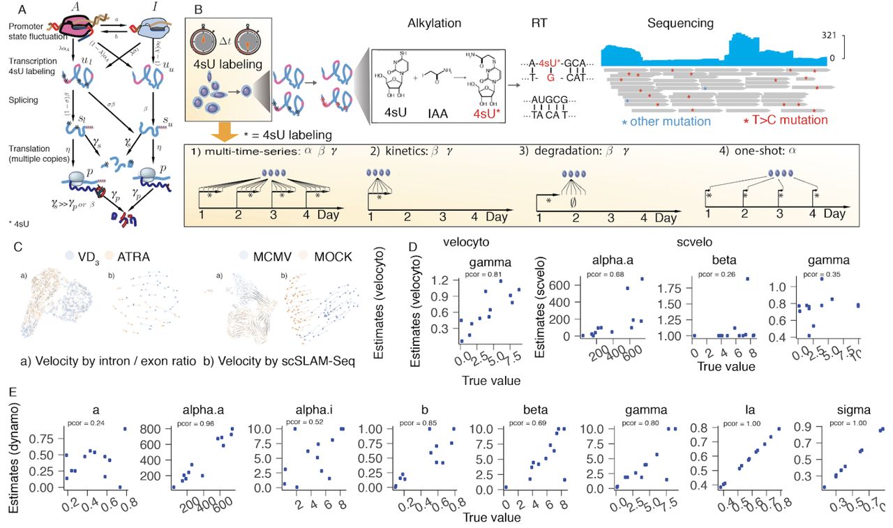
(A) The promoter state fluctuations, RNA transcription, splicing, translation, metabolic labeling and RNA/protein degradation model in dynamo. (B) Single-cell SLAM-seq workflow and experimental design for estimation of kinetic parameters in dynamo. (C) Transcriptional velocity based on scSLAM-seq reveal more consistent drug-induced expression changes in HL60 differentiation or cytomegalovirus infection (Erhard et al. 2019). (D) Performance of two existing velocity toolkits in estimating kinetic parameters based on the Gillespie algorithm implemented in dynamo. Annotated pcor values corresponds to pearson correlation between true value and estimated values (same as below). (E) Dynamo accurately and robustly infers all parameters involved in the full transcriptional kinetics.
For the purpose of estimating the full set of kinetic parameters, α(αA, αi), β, γs, which can be changed over the course of a biological process, it is ideal to have a “multi-time-series” of scSLAM-seq experiment data (case 1 in Figure 1B), in which single cell samples are collected at multiple time points each with a time course of 4sU treatment (see Method). The estimation method for this type of time-series data in dynamo builds upon a moment generating method where all parameters can be efficiently calculated through a matrix form of a set of moment generating functions, which makes it computationally efficient and trackable. However, it is often labor-intensive to collect such time courses and thus some model approximation are needed in practice. Although we cannot treat the transcription rate, α, as a constant because it directly relates to dynamic transcriptional regulation mediated through transcriptional factor binding, to a first approximation, we can assume constant RNA splicing or degradation rates (β, γ). These can be either measured through kinetics (a time-series of 4sU treatment to observe the accumulation of metabolically labeled mRNA) or degradation (a time-series after an extended 4sU treatment period to observe the decay of metabolic labeled mRNA) scSLAM-seq experiments. The kinetics or degradation experiments can be performed conveniently either at the beginning, at any meaningful time point in the middle, or at the end of the biological process under study. With the splicing or degradation rate estimated by this model, we then only need to harvest a single 4sU labeling time point at each stage of the time-course to infer the transcription rate α at that stage (Figure 1B, case 2/3). We note that dynamo can also handle data with only the metabolic labelling but no RNA splicing and similarly only RNA splicing but no metabolic labelling. In order to measure the protein velocity, we consider the case where single-cell splicing data and surface protein measurement from CITE-seq or the like are provided. Since no protein labeling strategy is applicable at this moment, estimation of protein velocity is based on a steady-state assumption in line with that used in the RNA velocity (See Method).
Dynamo circumvents key limitations of RNA velocity by taking advantage of controlled metabolic labeling of RNA species which is applicable to both steady states or transient states, and ensures that the parameters are estimated with the physical meaning of time considered. Importantly, our method estimates the transcription rate as it evolves at different time points. Existing methods lack this essential capability to estimate changing α, which we show in a simulation is vital as it can lead to the creation of new cell types in the phase diagram or the so-called “bifurcation” event in dynamic systems (Qiu, Ding, and Shi 2012) (see below, Supplementary Figure 1).

(A) Bifurcation plot of the spliced mRNA of gene 1, with respect to a changing parameter a defined in the method section. In the region of large a, the system contains five fixed points in total, three of which are stable (solid lines). The resting state of the cells is the symmetric fixed point (middle solid line), i.e. s1 = s2 as it has the largest attractor basin. As the bifurcation parameter a decreases because of external signals, the system goes to the region where there are three fixed points, two of which are stable. The original stable symmetric fixed point becomes unstable in this region, and thus the system bifurcates and relaxes to the two stable fixed points. (B) Phase plane of s1 and s2, with a = 15. The black dashed line is the nullcline when ṡ1 = 0, and the blue dashed line is the nullcline when ṡ2 = 0. The filled node corresponds to the stable steady state while the unfilled node the unstable steady state. (C) Velocity vectors computed by dynamo (and knn clustering. See method for more detailed discussions) for the unspliced mRNA. (D) Velocity vectors computed by dynamo for the spliced mRNA. (E) Velocity vectors computed by dynamo for the protein..
In order to demonstrate its power, we use plated-based scSLAM-seq to study the transcriptomic dynamics of HL60 cells differentiating into either monocyte-like or neutrophil-like cells by stimulating with hormone ATRA vs. VD3, respectively(Birnie 1988). Our results show that, in contrast to the velocity estimated from the unspliced/spliced read ratio, velocity estimated from metabolic labeled mRNA is more robust and consistent in revealing the magnitude and direction of transcriptional changes of HL60 cells following ATRA or VD3 treatment (Figure 1C), similar to other recent observations (Figure 1C, (Erhard et al. 2019)). This suggests that scSLAM-seq is a more direct and effective technique for quantifying the first derivative of RNA dynamics. In order to benchmark the robustness and accuracy of dynamo, we design a Gillespie simulation framework (Gillespie 1977) to model the differentiation of leukemia cell line, HL60. Although dynamo aims to learn eight parameters simultaneously in this benchmark, it performs favorably compared to RNA velocity (velocyto) and the recently improved velocity toolkit, scvelo without sacrificing computational efficiency (Figure 1D, E), demonstrating the power of the underlying theoretical foundation that dynamo builds upon.
Mapping the global vector field and potential landscape of single cells
A dynamic biological process can be regarded as the “movement” of cells across a high-dimension expression space, governed by the underlying gene regulatory network (GRN) (Mojtahedi et al. 2016) (Figure 2A). The proclivity of any configuration of GRN in a cell to generate a specific “movement” can be associated with the notion of “potential”, which is vividly represented by Waddington’s epigenetic landscape (Figure 2A) and guy-rope model (Creighton and Waddington 1958). Although Waddington’s epigenetic landscape is originally proposed as a metaphor, recent studies (Wang et al. 2010, 2011) provide a mathematical framework of defining an epigenetic landscape, where different “attractor” states appear and disappear when certain kinetic parameters of the system change slowly due to extrinsic or intrinsic signals (Supplementary Figure 1). While the vector field reveals the dynamics of a system, the potential landscape provides an intuitive global measure of the relative stability of the system and thus is useful to predict the probability that one cell type converts to another cell type. This can be used to define an optimal transition path to generate specific cell types for regenerative medicine.

(A) Biological processes are governed by underlying regulatory networks, which can be characterized by single-cell genomic measurements. Dynamic biological processes can be regarded as the “trajectory” in the high-dimensional expression (RNA and/or protein) space. The regulatory network determines the possible trajectories and final fates, which imposes the “potential” of cells in the expressional space. (B) Functional reconstruction of the velocity field from sparse velocity measurements and global mapping of potential landscape in single cells. Dynamo estimates the velocity of unspliced, spliced mRNA, and protein species from single cell transcriptomic or proteomic measurements enabled by metabolic labeling and transcriptome and proteome co-assays. The sparse, noisy and corrupted (indicated by the inaccurate velocity vectors (Ẋ*(t)) drawn in red) velocity measurements can be used to reconstruct the function  that describes the velocity vector field using the sparse vector field consensus approach (Jiayi Ma et al. 2013). Once the velocity vector function is inferred, the topology of the state space of the biological system can be estimated where the steady states (including attractor states (filled circles), ẋ(t) = 0, ẍ(t) < 0, and saddle points (unfilled circles), ẋ(t) = 0, ẍ(t) > 0), separatrices (lines or planes that separate the behavior of the velocity vector in the phase diagram, shown as the red line), nullclines (lines or planes where the velocity of one particular dimension is 0) can be estimated. Assuming the system as deterministic, Runge-Kutta method or line integration convolution algorithms can be used to quantify the entire path of the evolution of single cells from the very beginning to the final steady state in the full expressional space. Based on the principle of least action path, the potential landscape can be globally mapped, revealing the potential of cell differentiation or plasticity (Tang et al. 2017). It also provides the optimal transition path, associated work and the transition time that converts from one cell state to any other cell states in the entire state space (Tang et al. 2017). (C) Recovered vector field of simulated unspliced transcripts u1, u2 with dynamo. (D) Reveal topology of the phase diagram and predict full cell fate on Hippocampus (Kriegstein and Alvarez-Buylla 2009), hgForebrain (La Manno et al. 2018) and intestinal epithelium (Haber datasets) (Haber et al. 2017).
We have shown that velocity of unspliced RNA, spliced RNA and protein can be estimated with our kinetic model, which can predict cell states in the immediate past or future. But what about a state times in the more distal future or the past? Assuming the asymptotic deterministicity of the system (see Discussion), if we know the exact velocity of any point in the expression state space (that is, how a cell travels forward or backward given its current cell state), we can predict the cell state at an arbitrary time point. To make this plausible, mathematically it is desirable to have a function of the vector field for the entire state space. However, single cell measurements only offer us sparse and noisy vector sampling in the state space. Thus, the challenge is how to reconstruct a vector field robustly from sparse vector samples. Some pioneering work (Jiayi Ma et al. 2013) from computational graphics has shown that by defining a set of basis functions, it is possible to use the vector-valued reproducing kernels to learn the function of a vector field over the entire state space. Although those methods show impressive results on simulated data, it is not immediately clear how they perform when applied to biological systems where we have very limited samples and the velocity estimates are highly noisy.
In addition, although it is appealing to define “potential” for biological systems as it is intuitive and familiar from other fields, it is well-known that the definition of a potential function in open biological systems is controversial (Ping Ao 2009). In the conservative system, the negative gradient of potential function is relevant to the velocity vector by ma = −Δψ (where m, a, are the mass and acceleration of the object, respectively). However, a biological system is massless, open and nonconservative, thus methods that directly learn potential function assuming a gradient system are not directly applicable. In 2004, Ao first proposed a framework that decomposes stochastic differential equations into either the gradient or the dissipative part and uses the gradient part to define a physical equivalent of potential in biological systems (P. Ao 2004). Later, various theoretical studies have been conducted towards this very goal (Xing 2010; Wang et al. 2011; J. X. Zhou et al. 2012; Qian 2013; P. Zhou and Li 2016). Since we learn the functional form of the vector field, all those methods can be applied to map the potential landscape. The vector field reconstruction method itself can also directly learn the curl-free or divergence-free component of the vector field (Supplementary Figure 2). For this study, we operationally rely on our previous work to map the potential landscape numerically by taking the functional form of vector field and an assumed diffusion matrix as the input. This least action path (Figure 2B) based method(Tang et al. 2017) previously has been shown to glean insights in hematopoiesis, various carcinogenesis processes, including that of leukemia, breast cancer, lung cancer, etc, albeit mainly in the context of theoretical studies(Yuan et al. 2017).
In order to demonstrate the performance of vector field reconstruction by dynamo, we estimate the vector field based on the Gillespie simulation of leukemia cell differentiation, described above. We show that dynamo is able to convincingly recover the vector field which dissects two stable states near two side axes, each corresponding to either neutrophil-like state or monocyte-like state (Figure 2C). Interestingly, we are also able to identify one unstable state in the middle (Figure 2C). By using Runge-Kutta integration (RK) method (Kutta 1901) or Line Integral Convolution (LIC) (Cabral and Leedom 1993) that integrates along the path following the vector field to obtain the streamlines, dynamo recovers entire paths of single-cell evolution in the state space while also revealing the boundaries between these two cell states (Figure 2C).
Finally, we applied dynamo to a variety of published scRNA-seq datasets to predict the entire most probable evolution trajectories of cells during mouse hippocampus development, human forebrain differentiation, and the differentiation of small intestine epithelium cells (Figure 2D). The vector field revealed by dynamo uncovers interesting topology of the phase diagrams. For example, we see that the state space of the hippocampus is separated into multiple regions, each corresponding to an attractor basin for a particular cell type. We see that the phase diagram on the left are separated into two regions where the top one attracts to the Subiculum CA1/2/3/4 lineages while the bottom one the astrocyte cell state. Similarly, the top right corner, the middle bottom and bottom left regions are all separated nicely into regions that attracted to either CA1/2/3/4 cell type and granule, granule and OPC, and astrocyte and OPC cell type respectively. These results immediately offer testable hypotheses: if we perturb cells from any one of the attractor basins using CRISPRs-cas9 and other genome engineering methods, and divert them to another attractor basin, will those cells be destined to another cell types? For example, if we temporarily activate some astrocyte genes in cells from Subiculum CA1/2/3/4 lineages and effectively divert then to the attractor basin of astrocyte fate, will those cells eventually become astrocyte even after pausing the temporal activation of astrocyte genes?
Discussion
In this study, we show that it is plausible to build an analytical framework (Dynamo) capable of inferring the complete expression kinetics from temporal single cell measurements by taking advantage of metabolic labeling and proteome/transcriptome co-assay. It thus paves the way to build comprehensive biophysical models of biological processes. Our model overcomes several limitations of RNA velocity. The inclusion of scSLAM-seq (single-cell version of SLAM-seq and potential inclusion of CITE-seq) measurements for our model is widely applicable, allowing our approach to be immediately used to study various dynamical biological processes such as differentiation and tumorigenesis. Although currently we only implement scSLAM-seq with plate-based single cell protocols, we speculate that it is plausible to extend to Droplet-based approaches(Macosko et al. 2015) or microwell (e.g. seq-well (Gierahn et al. 2017) or Celsee® system) as a way of increasing the scale of the experiments. We further show that even with sparse sampling of velocity measurements, it is possible to robustly reconstruct the function that describes the velocity field, thus our method learns the transcriptomic vector fields from single cell measurements which reveals the motion of gene expression dynamics across the entire expression space. By moving forward or backward in time and integrating over the reconstructed velocity vector field, we can in principle predict the most probable cell state in arbitrary historical or future time points. Vector fields are widely used in various disciplines, we anticipate that techniques developed in other fields can also be adapted to study the dynamics, structure and topology of the reconstructed single cell vector fields.
We note that the prediction of cell fate is distinct from the pseudotime ordering in the sense that pseudotime ordering reflects central trajectory of state transition of a population of cells while our prediction reveals plausible dynamic evolution of each single cell in the state space. Pseudotime ordering is often nondirectional and we propose an empirical step-wise method that combines pseudotime with velocity we can automatically orient the learned graph of pseudotime trajectory (see Supplementary Method). However, it will be interesting to explore the possibility to learn directed graph from data with spliced and unspliced transcripts as well as other data-types with temporal dynamics directly.
Our model for predicting the historical or future states of single cells implicitly assumes a deterministic system, the cell fate under this perspective will eventually converge into fixed points (saddle points or attractors). Biological system is, however, intrinsically stochastic, the prediction of a single cell state with the reconstructed vector field is thus challenging in predicting long-range dynamics because of noise propagation. Nevertheless, this work foreshadows the possibility of predicting long-term trajectories of cells during a dynamic process. We also note that it is possible to study velocity vector in higher scales by predicting the average behavior of cell state transition for a population of cells which will render the predictions tolerant to the biological stochasticity. It is also an interesting future direction to formulate an entirely stochastic model to eliminate the deterministic assumption. As we previously showed that algorithms of information theory that takes advantage of velocity can be used to improve causal regulatory network inference (Qiu et al. 2018), the vector field reconstruction methods used here can also in principle be generalized to infer regulatory networks while reconstructing the functional form of vector field.
We recognize that the concept of “potential” for unconservative open biological systems is controversial and different formulations are proposed by various groups (Xing 2010; Wang et al. 2011; J. X. Zhou et al. 2012; Qian 2013; P. Zhou and Li 2016). Although in this study we chose a numeric algorithm we developed previously to map the potential landscape, our framework is generally applicable to all those different definitions as it learns the function of the vector field. For a dynamic biological process, the underlying regulatory network and thus the vector field may evolve over time. In principle, we should reconstruct the vector field at each time point which however impractically demands infinitesimal sampling of large number of cells over time. Nevertheless, one can reconstruct the vector field as a function of some slow variables (for example, extrinsic singling factors), emptomized by the Waddington’s landscape. Under this perspective, previously reported RNA velocity estimates (La Manno et al. 2018) and that learned by us have already projected onto the manifold with explicit slow variables (or components).
In this study, we specifically concentrate on introducing the theoretical foundations to predict cell states based on an inclusive model of gene expression dynamics, the functional reconstruction of vector field and global mapping of potential landscape. However, it will be interesting to validate those predictions of the entire dynamic trajectory during cell fate transition and the topology of the phase diagram or relative stability of cell states in a controlled system. For example, because we can predict cell dynamic evolution from any starting point in transcriptomic space, it will be interesting to perturb the system to states that normally are not populated, and show that cells indeed evolve as predicted from the vector field. Finally, the methods developed here will enable us to discover the boundaries of cell type transcriptomic states, the optimal path for reprogramming experiments, etc and ultimately leads to fundamental understanding of the mechanisms that drive cell fate transitions.
Material and Methods
Cell Culture
HL60 cells (ATCC® CCL-240™) were grown in RPMI 1640 medium (Gibco) at 37°C under 5% CO2, supplemented with 10% fetal bovine serum (Sigma) and 1% Penicillin/Streptomycin (HyClone). Cells were maintained below a density of 106 cells/ml. On the first day of the differentiation experiment, cells were seeded with 200,000 cells/ml on twelve well plates and are either treated with 1μM ATRA (all-trans-retinoic acid, Cat #R2625-100MG) or 1μM Vitamin D3 (Cat #PHR1237-500MG) to differentiate into either the neutrophil-like or monocyte-like cells. Cell differentiation status is confirmed by flow cytometry analysis of CD14 (Biolegend, Cat #367117) and CD11b (Biolegend, Cat #301309).
Bulk SLAM-seq time-series
To study the expression dynamics during differentiation, HL60 cells were induced to differentiate by either 1μM ATRA or 1μM Vitamin D3. Three biological replicates were collected at 0 hour, 14 hour, 36 hour and 96 hour after treated with either drug. 100mM 4sU were added to the wells and cells were labelled for 50 mins before collection. The collected total 21 samples were then subjected to the standard SLAM-seq protocol as stated by the manual from the Anabolic Module Kit (Lexogen, SKU: 061.24). Alkylated RNAs are then treated as single-cell samples to prepare SMART-seq2 library for sequencing according to a modified protocol (The Tabula Muris consortium et al. 2019).
scSLAM-seq
After treatment of ATRA or Vitamin D3 for 36 hours, HL60 cells were labeled in medium with 100mM 4sU (Lexogen) for 50 minutes at 37°C and sorted into lysis buffer (4μl, 0.5 U Recombinant RNase Inhibitor (Takara Bio, 2313B), 0.0625% TritonTM X-100 (Sigma, 93443-100ML), 1: 600,000 ERCC RNA spike-in mix (Thermo Fisher, 4456740) in 96-well PCR plates. All plates were frozen at −80°C until use. After thawing the plates to room temperature, to the lysed cells, 0.4 μL of 10x PBS and 0.4μL of alkylation mix (20mM IAA in DMSO) was added for a final alkylation reaction of 10mM IAA, 50% DMSO. Alkylation was stopped by adding 1.3 μL of 100mM DTT, incubating for 5 minutes at room temperature, Alkylated RNA was purified with 1.1 volume of Ampure XP beads and x2 washes with fresh 80 ethanol and eluted into an RNA elution buffer (3.125 mM dNTP mix (Thermo Fisher, R0193), 3.125 μM Oligo-dT30VN (Integrated DNA Technologies, 5’AAGCAGTGGTATCAACGCAGAGTACT30VN-3’), 0.5 U Recombinant RNase Inhibitor)). RT and the remaining library preparation was performed according to a modified version of Smart-seq2 (The Tabula Muris consortium et al. 2019). MiSeq (Illumina) was used to sequence the prepared libraries to generate paired-end read with 100 PCR-cycle. In total 349 cells are sequenced while 177 cells without 4sU labeling are used negative controls.
Dynamo: an inclusive model of gene expression dynamics
To enable the analysis of scSLAM-seq data, Dynamo is equipped with a command-line tool that implements existing best-practices to prepare the estimates of nascent or old RNA, spliced or unspliced transcript as well as protein abundance. At the core of Dynamo, it uses an inclusive model to model gene expression dynamics and estimate kinetic parameters.
Modeling the dynamic system using moment equations
The system shown in Figure 1A can be modeled using master equations (see Supplementary Method) when we have the multi-time-series samples (Case 1 in Figure 1B), which are PDEs (partial differential equations) characterizing the time evolution of the joint probability P(nuu, nul, nsu, nsl). Using the moment generating function technique, one could obtain the moments of any given order of the four species’ copy numbers, nuu, nsu, nul, nsl. In this study, we focus only on the first and the second moments, since the mean and variance computed from the data suffice for the estimation of all the parameters in the model.
The ODEs (ordinary differential equations) of the first moments are the same with those derived from a deterministic model (see next section):
 where
where  , and can be seen as the effective transcription rate. Note that these equations are not affected by the bursting frequency, if the ratio of a and b is held constant. Given enough temporal data of the four species, all the kinetic parameters can be estimated, except for a and b.
The ODEs of the second moments describe how variances and covariances evolve over time:
 note that
  , where 〈nul〉A and 〈nul〉I are the first moments of nul given that the promoter is active or inactive, respectively. The second moments of nuu and nul, in particular, give us enough information on the bursting frequency of the promoter and thus the estimation of a and b.
Modeling the dynamic system using ODEs
Similar to previous studies(Jia, Zhang, and Qian 2017; La Manno et al. 2018), the model for the dynamical system of transcription, splicing, and translation is formulated in terms of the following ODEs:
 where all the parameters are assumed to be constant, except for α, which is defined as a function of time (including the effect of external signals), and concentrations of proteins encoded by the transcription factors and directly related to the underlying gene regulatory network. In general, its form can hardly be modeled, and it requires a considerable amount of time-series data at multiple time points to estimate the parameters (Case 1 in Figure 1B). Alternatively, we can first estimate the constant parameters β, γ based on either one kinetic or one degradation experiment (Case 2, 3 in Figure 1B), and then estimate α locally for each cell with just one-shot labeling data, assuming α a constant in a short period of time (e.g., a few hours, compared to the time scale of the process of differentiation, which is around a few days) (Case 4 in Figure 1B).
Given a set of kinetic parameters, the velocities of a certain species of any given gene can be computed using the above ODEs. Furthermore, if we take the second derivatives w.r.t time for the spliced mRNA and protein, we acquire their accelerations (similar to that discussed in (Gorin, Svensson, and Pachter 2019)):

Taking the third derivative, we can also compute the jerk of protein based on the accelerations:

It is straightforward to generalize the above formulation to a system with n genes. For gene i:

The velocity, acceleration, jerk estimates in single cells from above can be then used to learn the function of the vector field in the entire expression state space.
Parameter Estimation
Most relevant studies estimate the degradation-related parameters (γ and δ) with a pseudo-steady state assumption, while either assuming β and η to be 1, or scaling the variables by β and η(La Manno et al. 2018; Gorin, Svensson, and Pachter 2019). When single-cell (or bulk) kinetics data using metabolic labeling (Hendriks et al. 2018; Erhard et al. 2019; Cao, Zhou, et al. 2019), for instance, scSLAM-seq, at multiple time points are available, it is feasible to further estimate β, γ, and δ for each gene using nonlinear least squares methods. In general, given m experimental data points y(1), y(2), …, y(m) at time points t(1), t(2), …, t(m) the least squares fitting method finds a set of parameters k that minimize the following loss function:
 where x(t, k) is the solution of the ODEs at the time point t, given parameters k.
Specifically, for the degradation experiment (Case 3 in Figure 1B), since samples are collected after pausing an extended 4sU labelling period, only the decay of pre-labelled transcripts will be observed while no new labeled transcripts will be generated, the transcriptional rate α is effectively 0, and the solution of the (labeled) unspliced mRNA is given by:
 where the splicing rate constant β can be estimated from the unspliced, labeled mRNA data in the degradation experiment, using the least squares fitting method. Then the solution of the spliced mRNA with 4sU labelling (with α is effectively treated as 0) is:

With a known β, parameter γ can be estimated accurately from the degradation data of the spliced, labeled mRNA. We can also determine the labeling rate λ by computing the ratio of the labeled and the total of the labeled and unlabeled mRNA. For proteins, since no labelling techniques exist at this point, so the pseudo-steady state strategy is employed to estimate δ/η, similar to that used by (La Manno et al. 2018; Gorin, Svensson, and Pachter 2019). Once we determine β, γ, δ/η, the velocities  and
and  can be computed based on the ODEs in the previous section. For data obtained from “kinetics” experiments, the parameters can be estimated all at once using the ODEs of the first moments introduced in the previous section.
The solution of the unspliced mRNA with a constant transcription rate λα, starting from time 0 (u(0) = 0), is:.

With a known β, α can be evaluated locally for each unspliced mRNA data u(i) for a short time period, using the data from the “one-shot” experiment:
 where t* is the duration of the labeling process. With an estimated α(i) and β, one can compute the velocity for the unspliced mRNA
  . We use clustering techniques, such as k-nearest neighbors and k-means, to reduce errors and obtain more consistent directions of the velocity vectors in the phase diagram for u1, u2, ., un.
In order to facilitate different usage cases, dynamo also supports estimating velocity with splicing only (data with only unspliced or spliced transcript counts) or labelling only (data with only labelled or unlabelled transcript counts) data using the pseudo-steady state assumption.
Data synthesis with Gillespie simulation of a two-gene bifurcation system
To test our method computationally, we simulated a system with two self-activating genes that mutually inhibit the transcription of each other (Figure 2A). The mathematical model is adapted from Qiu et al. (Qiu, Ding, and Shi 2012), with additional inclusion of RNA splicing, translation, protein degradation and metabolic labelling. The ODEs for the system are:
 where
where

To simplify the model, we assume that a1 = a2 = a, b1 = b2 = b, K1 = K2 = K, β1 = β2 = β, γ1 = γ2 = γ, η1 = η2 = η, δ1 = δ2 = δ.
As shown in Supplementary Figure 1A, the model leads to either a three-well or a two-well landscape, depending on the value of a bifurcation parameter a, which directly affects the transcriptional rate of the two genes. We assume that, initially, the system starts from the three-well landscape, where the majority of cells will reside in the middle well. Then a is changed so that the system goes to the bistable regime. The initially stable resting state now become unstable, and therefore the cells transition gradually to the two new stable fixed points (Supplementary Figure 1B). The simulation setup here effectively describes the differentiation of HL60 cells into either the monocyte-like or granulocyte like state under the treatment of ATRA or VD3.
To incorporate noise generated by the stochastic gene expression, we used the Gillespie algorithm (Gillespie 1977). The following table shows the propensity for each reaction:

At t = 0, 5, 10, 40, 100, and 150, we simulate the one-shot labeling experiment by introducing two labeled species: unspliced, labeled mRNA (w1, w2), and spliced, labeled mRNA (l1, l2). For the purpose of simplicity, in our simulation we assume all nascent mRNAs are labelled (i.e. λ = 1), and therefore the transcriptional rates for the unlabeled mRNA are set to 0, while that for the labeled mRNA are α1(p1, p2) and α2(p1, p2). The labeling duration t* = 1.
At t = 0 and 150, we simulate the degradation labeling experiment by first introducing 4sU labelling to the nascent RNA (similar to the above) for 10 units of simulation time, and then stop 4sU labelling (treat the transcriptional rates for the labeled species as 0) and watch for decay of the pre-labelled RNAs. We sample data at t = 0, 1, 2, 4, 8 after the pausing of 4sU labelling.
After estimating the kinetic parameters and predicting the local velocity of unspliced, spliced and protein measurement of single cells with Dynamo, it then relies on a set of mathematical techniques, Sparse Vector Field Consensus (sparseVFC) (Jiayi Ma et al. 2013), to functionally reconstruct the vector field, as described below.
Dynamo: Robust reconstruction of vector field from sparse single cell measurements
Vector field of expression space in single cells
In classical physics, including fluidics and aerodynamics, velocity and acceleration vector fields are used as fundamental tools to describe motion or external force of objects, respectively. In analogy, RNA velocity or protein accelerations estimated from single cells can be regarded as samples in the velocity (La Manno et al. 2018) or acceleration vector field (Gorin, Svensson, and Pachter 2019). In general, a vector field can be defined as a vector-valued function f that maps any points (or cells’ expression state) x in a domain Ω with D dimension (or the gene expression system with D transcripts / proteins) to a vector y (for example, the velocity or acceleration for different genes or proteins), that is f(x) = y. In two or three dimensions, a velocity vector field is often visualised as a quiver plot where a collection of arrows with a given magnitude and direction is drawn. For example, the velocity estimates of unspliced transcriptome of sampled cells projected into two dimensions is drawn to show the prediction of the future cell states in RNA velocity (La Manno et al. 2018). During the differentiation process, external signal factors perturb cells and thus change the vector field. Since we perform genome-wide profiling of cell states and the experiments performed are often done in a short time scale, we assume a constant vector field without loss of generality (See also Discussion). Assuming an asymptotic deterministic system, the trajectory of the cells travelling in the gene expression space follows the vector field and can be calculated using numerical integration methods, for example Runge-Kutta algorithm. In two or three dimensions, a streamline plot can be used to visualize the paths of cells will follow if released in different regions of the gene expression state space under a steady flow field. Another more intuitive way to visualize the structure of vector field is the so called line integral convolution method or LIC (Cabral and Leedom 1993), which works by adding random black-and-white paint sources on the vector field and letting the flowing particle on the vector field picking up some texture to ensure the same streamline having similar intensity. Although we have not discussed in this study, with vector field that changes over time, similar methods, for example, streakline, pathline, timeline, etc. can be used to visualize the evolution of single cell or cell populations.
Sparse vector field estimates from scSLAM-seq
With scSLAM-seq data and the computational framework mentioned above, in principle we can obtain vector field samples in either the unspliced transcriptome, spliced transcriptome, alternatively the nascent, old transcriptome in terms of metabolic labeling or proteome (the five axes of expression as we put it) space. Those spaces are often reduced into two or three dimensions for the purpose of visualization or interpretability, using PCA (principal component analysis) or UMAP(McInnes et al. 2018) (Uniform Manifold Approximation and Projection), etc. Although it is convenient to use two dimensional systems to demonstrate the method, the vector field reconstruction approach described below intrinsically handles high-dimensional data. Note that for reconstruction of the vector field, we can choose any one of the five axes as the reference frame to reconstruct independently or reconstruct them jointly. In particular, if we choose the unspliced transcriptome as the reference, we can learn the velocity vector field of unspliced transcriptome while ensuring the derivative of this velocity vector field (acceleration) satisfying the estimated velocity of spliced transcriptome, similarly, the second derivative (jerk) of the unspliced velocity vector field satisfying the estimated velocity of proteome.
To formally define the problem of velocity vector field learning, we consider a set of measured cells with pairs of current  and estimated future expression states
  , that is,
  , where D is the number of genes (or reduced dimension) and N is the number of cells. The difference between the predicted future state and current state for each cell corresponds to the velocity and we denote it as
  . We suppose that the measured single-cell velocity is sampled from a smooth, differentiable vector field f that maps from xi to yi on the entire domain
  . Normally, single cell velocity measurements are results of biased, noisy and sparse sampling of the entire state space, thus the goal of velocity vector field reconstruction is to robustly learn a mapping function f that outputs yj given any point xj on the domain
  based on the observed data with certain smoothness constraints (Jiayi Ma et al. 2013). Under ideal scenario, the mapping function f should recover the true velocity vector field on the entire domain and predict the true dynamics in regions of expression space that are not sampled. The discussion introduced above is based on velocity vector field but it can be similarly extended into acceleration vector field (Gorin, Svensson, and Pachter 2019), etc.
Vector-valued Tikhonov regularization of vector-field reconstruction in Reproducing Kernel Hilbert Space (RKHS)
In order to produce a robust algorithm that generalizes well to expressional regions unexplored by the sampling data, the learning procedure described above is formulated as a regularized optimization problem, which is chosen to operate in a RKHS (a functional space, rather than a Euclidean space, in which point evaluation is through a set of continuous linear functionals). In contrast to usual scalar functions, the function for vector field f is a vector-valued function. Thus, we used the vector-valued Tikhonov regularization(Тихонов 1943) in a RKHS, denoted as  , that minimizes the following regularized objective function with a kernel function Γ (Jiayi Ma et al. 2013):
 where the first term on the right side of the equation corresponds to the empirical error between the inferred future expression state f(xi) and observed future state yi and Δ is the operator of the loss, defined as Δ(f(xi), yi) = pi∥yi − f(xi)∥(0 ≤ pi ≤ 1 is the weight for cell i and ∥·∥ is the
  norm). According to the powerful Representer Theorem(Kimeldorf and Wahba 1970), The optimal mapping function of the above regularized problem has the form (Jiayi Ma et al. 2013):

Therefore, learning the optimal function of single cell vector field is equivalent to find a set of coefficients under the defined kernel function Γ, which is determined by the following equation:
 where
where  is the Gram matrix (a kernel matrix) which is an N × N block matrix with the (i, j)-th block Γ(xi, xj).
  is a DN × DN diagonal matrix, calculated by the Kronecker product between the diagonal matrix P = diag(p1, …, pN) and the D × D identity matrix ID×D. Finally,
  and similarly
  are DN × 1 vectors. Finding the optimal vector field function with the above strategy is convenient, however it needs to learn a kernel for every observed cell and thus poses serious computational and memory burdens for large datasets with its time complexity of O(N2) and space complexity of O(N3) (Jiayi Ma et al. 2013). In addition, this method also assumes there are no outliers in the input data. To resolve the two challenges, Ma et. al. (Jiayi Ma et al. 2013) introduces a sparse approximation and an EM algorithm, respectively.
Sparse approximation for robust high-dimensional expression vector field reconstruction
To solve the time and space burden for large datasets, Ma et al proposed a very efficient algorithm (Jiayi Ma et al. 2013; J. Ma et al. 2014) that aims to learn a suboptimal function fs(x) in a space  with a small set (e.g. 50) of basis functions is developed and defined as
 where the point set
  may not be a subset of the input single cell vector field samples. It has also been shown that simply random sampling of arbitrary points performs no worse than other sophisticated selection methods (Jiayi Ma et al. 2013).
According to the sparse approximation, a unique vector field function can be obtained by

The coefficient matrix  can be computed with the following formula
 where Ũ is an N × M block matrix with the (i, j)-th block
  :
:

Compared to the optimal solution f* which is a linear combination of the basis functions Γ(·, x1),⋯, Γ(·, xN) given by all the observed single cell vector field samples, the suboptimal solution fs relies on a linear combination of arbitrary M-tuples of the basis functions, which makes the algorithm a significant boost in terms of time and memory efficiency (time complexity is linear to the number of cells) while suffers negligible decrease in the accuracy of the recovered vector field.
In addition, an EM algorithm is also used to deal with the velocity measurement outliers. Basically, we associate the single cell velocity measurement i with a latent variable zi ∈ {0, 1} that we need to learn, where zn = 1 indicate an inlier that has Gaussian noise with zero-mean and uniform standard deviation σ and zn = 0 an outlier that has a uniform distribution of 1/a while a beining the volume of the gene expression space. Based on the above considerations, the likelihood of the EM model with parameter set θ is then defined as

The MAP solution of θ is estimated using Bayers’ rule which is solved by an interactive EM algorithm. During the E step, the P matrix of the probability of each single cell velocity measurement is an inlier can be computed by

During the M step, the parameters σ2, γ will be updated according to

With those considerations, the velocity field function is then learned with the sparse approximation mentioned above.
We note that the above discussion implicitly considers velocity vector field reconstruction for a particular reference basis from the five axis of the expression space. However, it is straightforward to extend this framework to simultaneously learn the velocity, acceleration and jerk vector field for both of the unspliced, spliced transcriptome (or alternatively new or old RNA in terms of metabolic labelling) and proteome at the same time, that is

Divergence-free or curl-free kernels for learning vector field
The velocity vector field for cells undergoing cell cycle often forms a loop while that for the differentiation, drug response or other biological processes more or less open lines. This is reminiscent of the divergence-free and curl-free vector fields, respectively, which are also used in various techniques to map the potential landscape for open biological system (Xing 2010; Wang et al. 2011; J. X. Zhou et al. 2012; Qian 2013; P. Zhou and Li 2016). It is possible to perform the vector field reconstruction by learning a convex combination of the divergence-free kernel Γdf and the curl-free kernel Γcf, where the divergence free and curl-free kernels takes the following forms (Jiayi Ma et al. 2013):
 in which σ is the bandwidth (by default, it is 0.8) and the combination efficient is set to be 0.5 by default in dynamo.
Dynamo: Mapping potential landscape of single cell
The concept of potential landscape is widely appreciated across various biological disciplines, for example the adaptive landscape in population genetics, protein-folding funnel landscape in biochemistry, epigenetic landscape in developmental biology. In the context of cell fate transition, for example differentiation, carcinogenesis, etc, a potential landscape will not only offers an intuitive description of the global dynamics of the biological process but also provides key insights to understand the multi-stability and transition rate between different cell types and quantify the optimal path of cell fate transition. Because the conventional definition of potential function in physics is not applicable to open biological system, we and others proposed different strategies to provide a biological equivalent by decomposing the stochastic differential equations into either the gradient or the curl component and uses the gradient part to define the potential. While it is still impossible to obtain the analytical form of the potential function, we are able to use an efficient numerical algorithm we recently developed to map the global potential landscape. This approach uses a least action method under the A-type stochastic integration(Shi et al. 2012), a method that reconciles the “noise effects” resulting from using different stochastic integration methods, for example the predominant Ito or Stratonovich method, which leads to the incompatibility of fixed points under different noise levels.
To globally map the potential landscape Ψ(x), the numerical algorithm (Tang et al. 2017) takes the vector field function f(x)(in terms of kernel basis in our case) as input and consists of the following key steps:
Find the fixed points under consideration by solving the f(x) = 0 with the Newton iteration method.
Classify all the fixed points into two groups by calculating the eigenvalues of the linearized Jacobian matrix in their neighborhood: stable fixed points (no eigenvalue with positive real part) and unstable points (at least one eigenvalue with positive real part).
Choose a saddle point as reference. Start from the points in a small neighborhood of the saddle point s*, and follow the vector field function f(x) to find all the stable fixed points reached, x*. Calculate the potential difference ΔΨ between the saddle point and the stable fixed points by the least action method with the following equation,
 where A corresponds to the A-type stochastic integration, S(s*|x*) is equal to the potential difference between s* and x* which is minimization of the action function and is defined as
where the two infimum basically means that we want to find a path that minimizes the travelling time in the gene expression state space while ensuring it starts from s* and end up at x*. The action function ST[x]|A is defined as,
where the stochastic integration here is transformed into I (Ito) type and the time is discretized into K segments with T1 = t1 < ⋯ < tk < ⋯ < tK = T2, each interval being dt and xk = x(tk). Finally D is the diffusion matrix and we assume it as a diagonal matrix with the dimension or genes in the expression space.
where A corresponds to the A-type stochastic integration, S(s*|x*) is equal to the potential difference between s* and x* which is minimization of the action function and is defined as
where the two infimum basically means that we want to find a path that minimizes the travelling time in the gene expression state space while ensuring it starts from s* and end up at x*. The action function ST[x]|A is defined as,
where the stochastic integration here is transformed into I (Ito) type and the time is discretized into K segments with T1 = t1 < ⋯ < tk < ⋯ < tK = T2, each interval being dt and xk = x(tk). Finally D is the diffusion matrix and we assume it as a diagonal matrix with the dimension or genes in the expression space.Repeat step 3 for all saddle points. Assign relative potential difference between the saddle points if they reach a common stable fixed point.
For any other points in state space, follow the vector field f(x) to find the fixed point it reaches. Obtain their potential difference by the least action method.
With the calculated potential values, the relative probabilities between cell states can be calculated by
, which reveals the relative stability between cells.


Code availability
Dynamo (version: 0.0.1) is implemented as a python package and is available through GitHub (https://github.com/aristoteleo/dynamo-release). Notebooks for reproducing all figures in this study and tutorials of Dynamo usage cases are also available through GitHub (https://github.com/aristoteleo/dynam-onotebooks).
Supplementary method
Master equations of stochastic gene expression dynamics
Since the promoter has two states: active and inactive, we write the master equation in terms of the conditional probability given a promoter state. For example for the inactive promoter state:

The master equation for the active promoter state can be written in a similar fashion, by substituting I with A, and for the last line, change −b to a. Then we can define the moment generating function as:
 where s can either be A or I. By applying the moment generating function to the master equations, one can convert them to ODEs of moments of any order.
Integration of pseudotime ordering and velocity measurements
We used a step-wise method to integrate pseudotime ordering with velocity to automatically assign the direction of the learned trajectory. Let X be the input data and V be the corresponding velocity. The following steps are taken to create a directed graph.
construct k-nearest neighbor using FLANN (using k = 10)
compute transition probability by
where corr is the Pearson correlation coefficient between two vectors,compute transition probability by
run DDRTree (Qi Mao et al. 2015; Qiu et al. 2017) or L1-graph algorithm(Q. Mao et al. 2017; Cao, Spielmann, et al. 2019) on X and get centers Y, assignment matrix R, and undirected tree T. Compute the transition probability among
find segments of T and denote the kth segment by sk = sk,1, …, sk,m.
calculate the probability of the segment by first order Markov assumption:
To avoid the issue of numeric computation, log function is used as
Similarly, we can compute
for the kth segment.the direction of the k–th segment with the maximum transition probability is used
collect directions of all segments and form the directed tree.


AUTHOR CONTRIBUTION
X. Q., Y. Z., L. W. and J. X. developed the model and theory. X. Q., D. Y., S. H., J. R., S. D. and J. S. W. designed the experiments. X. Q., D. Y., S. H., J. R. performed the experiments. X. Q., Y. Z., L. W., R. Y., S. X., Y. M. performed the analysis. X. Q., J. X., J. S. W. conceived the project. All authors wrote the manuscript.
COMPETING INTERESTS
The authors declare no competing financial interests.
ACKNOWLEDGEMENT
We would like to thank Jiayi Ma, Tatsu Hashimoto for technical discussion on recovering vector field and potential function, Alex Ge, Luke Gilbert for helps on culturing HL60 cells and developing scSLAM-seq, Kara Mckinley and members of the Weissman lab for discussion and comments on this work.


