

Abstract
Kernel Current Source Density (kCSD), which we introduced in 2012, is a kernel-based method to estimate current source density (CSD) from extracellular potentials recorded with arbitrarily placed electrodes. Estimating reconstruction errors in CSD has been an outstanding challenge. To address it, here we revisit kCSD and explore its mathematical underpinnings. First, we quantify the information that can be recovered from extracellular recordings for a given setup, by introducing eigensources — a set of basic CSD profiles, which form the basis of estimation space. Next, we investigate the effect of relative placement of basis sources and electrodes on the reconstruction fidelity. We show that the correct distribution of sources is crucial for the reconstruction, in particular, CSD reconstruction is possible even for badly misplaced electrodes. We also introduce L-curve, a new method for choosing reconstruction parameters, in addition to the previously used cross-validation. Finally, we propose two types of diagnostics of reconstruction veracity, error propagation map and reliability map. For any given setup, the error propagation map indicates how the electrode noise propagates to the reconstructed CSD and the reliability map illustrates the point-wise reliability of kCSD estimation. The kCSD method and the additional techniques introduced here are implemented in kCSD-python, a new Python package provided under an open license. kCSD-python’s features and usage are highlighted with a jupyter notebook tutorial. This new tool can perform CSD estimations for 1D, 2D, and 3D electrode setups, assuming distributions of sources in a tissue, a slice, or in a single cell.
Introduction
Multisite recording of extracellular potential is a popular technique in neuroscience. The obtained potential reflects activity of underlying neural network and is directly related to the distribution of current sources along the active cells (current source density, CSD). The relation between the CSD and recorded potential, while occasionally contested [Bédard and Destexhe, 2011], overall is well established and trusted in experimental and analytical practice [Buzsáki et al., 2012, Einevoll et al., 2013, Gratiy et al., 2017]. Due to the long range of electric potential [Łęski et al., 2007, Hunt et al., 2011, Lindén et al., 2011, Łęski et al., 2013] it is useful to estimate the current sources. Several methods have been introduced to estimate current sources since 1950s [Pitts, 1952, Nicholson and Freeman, 1975, Pettersen et al., 2006, Łęski et al., 2007, 2011]. In 2012 we proposed a non-parametric method of CSD estimation which we called kernel CSD method (kCSD, [Potworowski et al., 2012]). Here we revisit this method with three aims in mind. First, to present a new Python based toolbox, which allows kCSD reconstruction of current sources for data from 1D setups (laminar probes and equivalent electrode distributions), 2D (planar MEA, multishaft silicon probes, Neuropixel or SiNAPS probes, etc), and 3D electrode setups (Utah arrays, multiple electrodes placed independently in space with controlled positions), where the sources are assumed to come from tissue (kCSD) or from single cells with known morphology (skCSD). Fig. 1 shows the different experimental scenarios for which this software is applicable. Second, using the new software, we investigate the properties of some mathematical structures arising in the context of practical experimental studies. Third, we introduce several new conceptual tools which will facilitate CSD estimation and knowledge extraction from the data.

Overview of experimental contexts where kCSD-python is applicable. 1D setups such as A) laminar probes and equivalent; 2D setups, such as B) multishaft silicon probes, Neuropixel or SiNAPS probes, or D) planar MEA; 3D electrode setups, such as multiple multishaft silicon probes, Utah arrays, multiple electrodes placed independently in space with controlled positions, where the sources are assumed to come C) from tissue (kCSD) or E) from single cells with known morphology (skCSD). For description of parameters see Methods.
Our plan is as follows. We first review the basic relations between the relevant physical quantities we study and we set up the computational framework. Then we study the central quantities involved in estimation of the sources from the measurements. We follow this with introduction of L-curve estimation of optimal reconstruction parameters and reliability maps for the study of reconstruction accuracy. Finally, we provide an overview of the new software package which was used for the presented analysis and illustrate the new concepts introduced here.
Current source density and local field potential
The extracellular potential that we measure is a consequence of ion motion in the tissue which is driven by ionic currents through the ion channels embedded in neuronal and glial membranes, as well as capacitive currents arising in response to potential gradients across the membrane. From the perspective of extracellular medium it seems as if the current was disappearing or appearing from inside a cell, which is why we talk about current sources and sinks. The distribution of these current sources is called the current source density (CSD) and its relation to the extracellular potential is given by the Poisson equation
 where C is the CSD, V is the extracellular potential, and σ — the conductivity tensor. Thus, if we knew the potential in the whole extracellular space, we could easily compute the CSD. On the other hand, knowing CSD in the whole space, we can compute the extracellular potential. Assuming isotropic and homogeneous tissue the Poisson equation reduces to
 which can be easily solved:

In more complex situations when σ depends on position and direction, and we have non-trivial boundary conditions, one must resort to numerical integration. This can be done Ness et al. [2015], Næss et al. [2017] but in the following we will assume constant scalar σ (homogeneous, isotropic medium). The reason is that more general models of tissue conductivity do not affect the following discussion and results but they would make presentation more cumbersome. In practice, they only affect the relation between the basis functions in the space of CSD and potential,  and bj in what follows. In the provided package this is one Python function that needs to be replaced.
Careful discussion of the meaning of the CSD and derivation of the relations between CSD and the potential can be found in Stevens [1966], Nicholson [1973], Gratiy et al. [2017]. Discussion of physiological sources of the extracellular potential can be found in the reviews by Buzsáki et al. [2012], Einevoll et al. [2013].
Kernel Current Source Density and prior estimation methods
Pitts [1952] observed that the Poisson equation relating the extracellular potential to the CSD can be used to estimate CSD from measurements. He used this observation to examine the distribution of currents and sinks in the spinal cord. His approach, which we call traditional CSD method, was based on direct numerical approximation to the second derivative in equation (2). Pitts’ approach with small modifications was used for more than half a century and is still in use today. In 2006, Pettersen et al. [2006] proposed a model-based approach to estimate CSD. The inverse CSD (iCSD) method which they introduced for analysis of laminar recordings assumed a parametric model of CSD with the recordings used to compute model parameters. Some advantages of this approach were explicit inclusion of assumptions regarding physical properties of the tissue conductivity and the properties of sources in the directions not probed. Inverse CSD facilitates testing the influence of these uncontrolled factors on the estimated CSD. It was extended to 2D and 3D recordings [Łęski et al., 2007, 2011], however, it still required recordings on regular rectangular grids (although see Wójcik and Łęski [2010]) and did not compensate for the measurement noise. Potworowski et al. [2012] proposed how to overcome these limitations generalizing iCSD to the kernel CSD (kCSD) method. It was later studied from the general perspective of discrete inverse problems by Kropf and Shmuel [2016].
Kernel CSD estimation is conceptually a two-step procedure. First, we do a kernel interpolation of the measured potential which gives V (x) in the whole space. This is obtained with the help of a symmetric kernel function, K(x, x′), so that
 where xj, j = 1, …, N, are electrode positions. The regularized solution, which makes correction for noise, is obtained by minimizing prediction error
 which gives
 where V is the vector of measured potentials, λ is regularization parameter, the norm
  is discussed in the Methods section, and

To simplify the notation and bring the discussion closer to our numerical implementation we shall consider estimation at an arbitrary discrete set of points yi, with i = 1, …, W. Further, in matrix representations of operators we shall assume the variables taking the values of electrode positions, xj, j = 1, …, N, or the values of estimation points, yi, i = 1, …, W. In the latter case we shall underline the matrix. So a single underline means rows are numbered by estimation points, and columns are numbered by electrode positions. Double underline means that both rows and columns are numbered by estimation points. The variable which takes value at estimation points can usually be also read as a free variable. For example
 or
or  . Usually these two viewpoints should be interchangeable, if not, specific use should be clear from the context. For example, when we discuss software implementation, only the first (discrete) view is applicable.
With this notation, our estimation of the potential in the whole space is

Once we estimate the potential we must shift the obtained solution to CSD space. This is easiest to understand in 3D where we can simply plug this solution into the Poisson equation (1), and compute CSD everywhere. In the general case this can be achieved with a second function, which we call cross-kernel,  . With these functions the resulting CSD estimation is given by

In practice, to identify relevant K and  , we introduce a large basis of CSD sources spanning the space of interest,
  , and corresponding basis in the potential space, bj(x), and construct our kernels from these basis functions [Potworowski et al., 2012]. We review the details of kCSD method in the Methods section.
The challenges of the method are how to construct K and  , how to select the relevant parameters, and reliability of the estimation. In the following we address all these issues conceptually and computationally with the provided open package, kCSD-python.
Results
In this paper we introduce the kCSD-python package, a novel implementation of the kernel Current Source Density method. It is distributed under an open license (3-Clause BSD License) and is available on GitHub (https://github.com/Neuroinflab/kCSD-python). The package contains a set of tools for kCSD analysis, for validation of the results of analysis, and extensive tutorials implemented in jupyter notebook to familiarize the user with its usage. It allows the user to analyze their own electrophysiological recordings or to explore the method with data generated in silico.
In this section we introduce several tools to facilitate conceptual and practical under-standing of the reliability of CSD analysis. First, we discuss spectral decomposition of the kCSD and introduce the concept of eigensources. Then we study the effects of relative placement of the basis, the electrodes and sources on reconstruction fidelity. We show that when the basis is placed in the region containing the true sources, reconstruction can be performed even if the signal is picked away from the source. Next we discuss parameter selection focusing on the L-curve approach which we introduced in the package along the previous cross-validation approach. Finally, we introduce reliability maps as a heuristic tool to build intuition about the power of any given setup to resolve the CSD.
We close this section with an extensive tutorial overview of the kCSD-python package. Its goal is to show how to use this package to perform CSD analysis, how to apply the provided analysis tools, and to validate the results. We first consider a regular grid of ideal (noise-free) electrodes, where we compute the potentials from a known test source (the ground truth). We then use these potentials to reconstruct the sources which we compare with ground truth (Basic features). Then, we explore the effects of noise on the reconstruction and test the robustness of the method (Noisy electrodes). In the final part of the tutorial we look at how the errors in the estimation depend on the sources and the electrode configuration by testing the effects of broken electrodes on reconstruction (Broken electrodes).
Spectral decomposition for kCSD and regularization
Let us reconsider the construction of kCSD (see Methods). In kCSD we estimate CSD in space  span by a large, M-dimensional basis,
  . However, our experimental setup imposes constraints which force our model to an N-dimensional subspace where the estimation really takes place, with N ≪ M. To understand the structure of this smaller space we can decompose the operator K, eq. (25), acting on the measurements. We can take advantage of the symmetry and positivity of K matrix which guarantees existence of eigendecomposition

Then the kCSD reconstruction for a set of measurements V, eq. (27), is

Since wj are orthogonal we have

Thus wj are the natural ‘eigenmeasurements’ corresponding to individual CSD profiles,  , accessible to the given setup when specific basis
  is assumed. Moreover, it is easy to see that the CSD profiles
 actually form the basis of estimation space, we call them ‘eigensources’. Since kCSD method is self-consistent, in the absence of noise, we see that the potential at the electrodes generated by
  is
is

It leads to reconstructed CSD
 which is equal to
  for λ = 0.
A natural question appears as to what happens to the missing M − N dimensions. The answer is that they are projected onto 0 (annihilated). It is possible to construct them explicitly. Starting with the basis of N eigensources we can expand it within  by Gram-Schmidt orthogonalization. This construction breaks
  into two orthogonal subspaces, one of which spans all the sources which can be recovered with a given setup, the other contains all the sources which are annihilated.
Let us now investigate this decomposition in an example. Here we study spectral properties of the simplest 1D case with regularly distributed electrodes. We consider M = 2k, k = 0, 1, …, 9 basis sources distributed uniformly in [0, 1] and the number of electrodes is N = 12. This means that K is 12 × 12 and there are 12 eigensources. Fig. 2.A) shows the eigenspectrum of K for growing basis size, M = 2, 8, 16, 512. As we can see, the spectrum of K quickly stabilizes and already for M = 16 it is very close to that for M = 512, so it is almost asymptotic. Approach to asymptotic values is illustrated for the leading eigenvalue which is plotted as a function of M in Fig. 2.B). Fig. 2.C-N)) show all the 12 eigensources,  , eq. 5, for the same basis. As we can see, in the degenerate cases of M < N only M eigensources are non-trivial and we can see that they are approximations to asymptotic sources. Eigensources for M = 16 are very close to those for M = 512 so it seems to indicate that as long as the number of basis sources, M, is larger than the number of electrodes, N, for regular distribution of electrodes and basis sources covering the same region, the number of basis functions is not a limiting factor of the reconstruction. On the other hand, as we observed before, every reconstruction is a linear combination of the eigensources, thus the only things which can be reconstructed are linear combinations of the profiles shown in Fig. 2.C)-N).

Demonstration of spectral properties of kCSD method for simple 1D case with 12 regularly distributed electrodes on the interval [0, 1]. A) Eigenvalues obtained from the decomposition of K for different number of basis sources (M=2, 8, 16, 512), B) Shows the first eigenvalue in the function of growing number of basis, C–N) Shows 12 eigensources (products of  and all the eigenvectors), which produce the inverse solution in kCSD method. Different curves represent eigensources estimated for different M.
Observe that for electrodes placed on a regular grid the set of eigensources forms a Fourier-like basis. This is in line with other results in discrete inverse problems Hansen [2010] although here we do not consider singular value decomposition of resolvent as is usually done (see e.g. Kropf and Shmuel [2016]). This brings to mind the sampling theorem Oppenheim et al. [1996], except here we measure one quantity (the potential) and reconstruct another (CSD). In the sampling theorem we reconstruct a continuous signal from discrete samples. This in particular shows that there would be a range of spatial frequencies within which reconstruction is efficient and beyond which it will increasingly fail. While this is a linear oversimplification it captures the intuition well. For an alternative view of this observation see Fig. 2 of Cserpan et al. [2017].
Note that we can perform similar studies for arbitrary setups. Once they are no longer regular, the basis of eigensources may deviate from Fourier arbitrarily. This can be easily studied with the kCSD-python package introduced here for any given setup used experimentally.
The effects of relative placement of basis, electrodes, and sources, on reconstruction fidelity
In CSD analysis it is usually assumed that the electrodes probe the region of interest well and that the sources to be reconstructed are within the space span by the electrodes. It has usually been our tacit assumption so far, in this and previous papers. However, this need not necessarily be so. First, in many experiments carried in the past and at present, the number of electrodes is small, we often probe complex extended structures with laminar probes, etc. Second, it is relatively common to record away from the source. For example, imagine in vivo study where we target a specific structure where activity is expected yet post-experimental histology shows the probe was misplaced. Can we learn anything of value about the sources of interest in such a case?
To address this question here we consider a 1D Gaussian source centered at 0.25, which is essentially nonzero on interval [0, 0.5], where the interval [0, 1] is a metaphor for the whole brain. We then consider nine cases with three different distributions of 12 electrodes on intervals [0, 1] (‘within the whole brain’), [0, 0.5] (covering only the region where the source is non-zero), [0.5, 1] (badly misplaced probe), and three different distributions of basis sources, spanning the intervals [0, 1], [0, 0.5], [0.5, 1] (Fig. 3). The different placements of basis sources are a metaphor for the prior knowledge from expert insight of where we anticipate the sources. Here, the width of the basis source, R, was selected through cross-validation for the first case and used throughout, λ = 0 and no noise was assumed.

Demonstration of kCSD reconstruction for different relative placement of basis sources and electrodes for simple 1D Gaussian source in the absence of noise. Width of the basis source, R, was selected through cross-validation for the first case (A) and used throughout. Columns represent results for three different distributions of basis sources: left — centers of basis sources distributed uniformly on interval [0, 1], middle — interval [0, 0.5], right — interval [0.5, 1]. Rows represent different distribution of electrodes: top — electrodes span the interval [0, 1], middle — interval [0, 0.5], bottom — interval [0.5, 1]. Black dots represent electrode positions, continuous line — ground truth (TrueCSD), dashed line — CSD estimated with kCSD method.
In Fig. 3, consider the first row, where the electrodes span ‘the whole brain’. In that case, if we distribute the basis sources throughout the brain (left column, panel A) or through the region where the true sources were placed (middle column, panel B), the reconstruction is faithful. However, if we distribute the basis sources in the right half of ‘the brain’, away from the true sources (Right column, panel C), kCSD fails miserably trying to reconstruct the source from the measured potentials in the place where there is nothing. This is to be expected. Interestingly, when the electrodes are placed on the right half, completely outside the region containing the true sources, if we place the basis sources so that they cover the region where the true sources are located the reconstruction, while misshapen, does indicate the location of sources (Panels G and H). Moreover, if we have expert knowledge which tells us to expect the source in the left half, and we accordingly place the basis sources only there, the reconstruction is actually remarkably faithful (Panel H). These results indicate that it is worthwhile to attempt reconstruction even in cases with misplaced electrodes, as long as we know relative distances between the electrodes and we have reasons to speculate the source being reconstructed to be in a restricted region.
Since noise-free data are not realistic it is interesting to investigate how noise affects these results. In a real life scenario we would always tune the parameters R, λ from data using cross-validation or L-curve method (next section). Fig. 4 shows reconstructions in the same nine cases as before for data which have been contaminated with additive noise. We show results obtained when optimal parameters where selected with cross-validation or with L-curve method in every case. As we can see, even though the results degrade when compared with the noise-free data, in all cases regularization improves the reconstruction, often providing useful information. Interestingly, in the case where we record outside the region of interest but where the basis spans ‘the whole brain’, L-curve gives a reasonable estimate while cross-validation fails. Note that this is accidental. Our tests show that in difficult cases one or the other approach to parameter selection may give better results.

Demonstration of kCSD reconstruction for different relative placement of basis sources and electrodes for simple 1D Gaussian source. Here we assume measurement noise, thus cross-validation and L-curve methods were used to select regularization solution parameters R, λ. Columns and rows — see previous figure. Black dots represent electrode positions, continuous line — ground truth (TrueCSD), dashed line — CSD estimated with kCSD method, dotted line — L-curve estimation.
Parameter selection
An important part of kCSD estimation is selection of parameters, in particular the regularization parameter, λ, but also the width of the basis source, R. Previously we proposed to use cross-validation. Here we also apply L-curve approach [Hansen, 2010, Kropf and Shmuel, 2016] for regularization. Both these methods are implemented in the provided Python package.
Cross-validation
To select parameters using cross-validation [Potworowski et al., 2012] we consider a range of parameter values, λ ∈ [λ0, λ1]. For any test value λ we select an electrode i = 1, …, N and ignore it. With eq. (24) we build a model from remaining measurements,  , and use it to predict the value at the ignored electrode,
  .
.
Here
 where the minimizing vector
 and where ′i means i-th column and row are removed from the given matrix.
We repeat this for all the electrodes i = 1, …, N and compare predictions from the remaining electrodes against actual measurements:

For final analysis, λ giving minimum prediction error is selected. It is worth checking if the global minimum is also a local minimum. If the λ selected is one of the limiting values this may indicate that extending the range of λ might result is more optimal result or that the problem is ill-conditioned, for example too noisy, etc, and we are either underfitting or overfitting, as we discuss below for the L-curve.
L-curve
Consider the error function, Eq. (23), which we minimize to get the regularized solution,  . It is a sum of two terms we are simultaneously minimizing, prediction error
 and the norm of the model
 weighted with λ. Taking λ = 0 is equivalent to assuming noise-free data. In this case we are fitting the model to the data, in practice, overfitting. On the other hand, taking large λ means assuming very noisy data, in practice ignoring measurements, which results in a flat underfitted solution. Between these extremes there is usually a solution such that if we decrease λ, the prediction error, ϱ, slightly decreases, while the norm of the model, η, increases fast, or the opposite, Fig. 5D.

An example of the L-curve method for estimating kCSD parameters. A) The red points represent the potential used for CSD reconstruction. The black points show the electrode positions. The ground truth is shown in panel C with the red dashed curve. The measurement was simulated by adding small random noise to all the electrodes (32 values taken from a uniform distribution). The blue line shows a kernel interpolation of the potential which is the first step of kCSD method. B) L-curve plot for a single R parameter. The apex of the L-curve is numerically computed from the oriented area of directed triangles connecting the point on the L-curve with its two ends. C) Comparison of the true CSD and kCSD reconstruction for parameters obtained with L-curve regularization. D) Etimation of L-curve curvature with triangle method (see the Methods).
This is apparent when the prediction error and the norm of the model are plotted in the log-log scale. This curve follows the shape of the letter L, hence the name L-curve [Hansen, 1992]. Several methods have been proposed to measure the curvature of the L-curve and to identify optimal parameters [Hansen et al., 2007]. In kCSD-python, we have implemented the triangle area method proposed by Castellanos et al. [2002].
To illustrate this method in the context of CSD reconstructions, we study an example of 1D dipolar current source with a split negative pole (See Fig. 5C, True CSD, red dashed line). We compute the potential at 32 electrodes (Fig. 5A, C, black dots) with additive noise at every electrode. Notice that if we reliedwanted to interpret the recorded potential directly (Fig. 5A, red dots) it is difficult to discern the split negative pole. Fig. 5D shows the estimated curvature for our example as a function of λ. The optimal value of λ is found by maximizing the curvature of the log-log plot of η versus ϱ, Fig. 5B. The red dot in Fig. 5B, D, indicates the ideal λ parameter for this setup obtained through the L-curve method.
Several methods have been proposed to measure the curvature of the L-curve and identify optimal parameters [Hansen et al., 2007]. We adopted the triangle area method proposed by Castellanos et al. [2002]. To distinguish between convex and concave plot, clockwise directed triangle area is measured as negative. Fig. 5D shows this estimated curvature for our example as a function of λ.
Fig. 6 compares results of parameter tuning and reconstruction by cross-validation and L-curve method. The top panel shows the estimation error between the reconstruction and the ground truth (known model data) for the two approaches as a function of increasing measurement noise simulated. The bottom panel shows which λ is being selected by both methods as the noise is increasing. The mean and the errors were obtained for 10 different realizations of noise. As we can see, the two methods give consistent results for low noise. For increasing noise, in this case, the L-curve tends to indicate lower λ values which here gives a slightly bigger error. However, it is computationally faster.
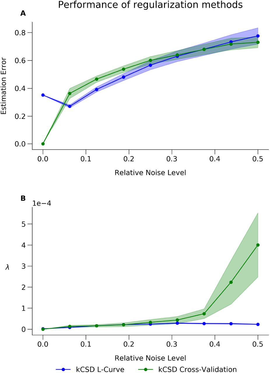
Comparison of parameter selection using cross-validation and L-curve method with the addition of noise A)The estimation error value is calculated as root mean square error between normalized true CSD and estimated CSD (normalized to maximum value) obtained either by using L-curve (blue) or by using cross-validation (green) B) The corresponding ideal λ parameter selected. For both these of methods λ increases with the added noise. Blue and green ribbons indicate standard deviation of the RMS around mean λ computed from 10 different noise realizations.
Reconstruction accuracy
With kCSD procedure one can easily estimate optimal CSD consistent with the obtained data. However, so far we have not discussed estimation of errors on the reconstruction. Since the errors may be due to a number of factors — the procedure itself, measurement noise, incorrect assumptions — one should consider several approaches to this challenge.
First, to understand the effects of the selected basis sources and setup, one may consider the estimation operator  and the space of solutions it spans. As we discussed above, this space is given by the eigensources, eq. (5). The orthogonal complement of this space in the original estimation space,
  , is not accessible to the kCSD method. The study of eigensources facilitates understanding which CSD features can be reconstructed and which are inaccessible.
Second, to consider the impact of the measurement noise on the reconstruction, for any specific recording consider the following model-based procedure. Reconstruct CSD from data with optimal parameters. Compute potential from estimated CSD. Add random noise to each computed potential. The noise could be estimated from data, either as a measure of fluctuations on a given electrode for a running signal, or from variability of evoked potentials. Then, for any realization of noise, compute estimation of CSD. The pool of estimated CSD gives estimation of the error at any given point where estimation is made.
This computation can be much simplified by taking advantage of the linearity of the resolvent,  . Then, the i-th column (Ei) represents contribution of unitary change of i-th measured potential (the i-th element of the vector V) to the estimated CSD
  . As the contribution is proportional to the change, the column can be considered an Error Propagation Map for i-th measurement (Fig. 7.A). Note that these vectors (the columns of resolvent, Ei) also happen to form another basis of the solution space, an alternative to the basis of eigensources.

A) Error propagation maps for 3 × 3 regular grid of electrodes. Every panel represents the contribution of the potential measured at the corresponding electrode marked with a black circle (∘) to the reconstructed CSD. Every other electrode is marked with a black cross (×). B) Map of CSD measurement uncertainty for 3 × 3 regular grid of electrodes. The CSD measurement uncertainty is represented by variance of the CSD reconstruction caused by the uncertainty in measurement of the potentials. It is assumed that measurement errors for electrodes are mutually independent and follow standard normal distribution  . Location of electrodes is marked with red crosses (×).
If εi is an error of i-th measurement, then its contribution to  is εiEi. Moreover, if the measurement errors follow multivariate normal
 then
then
 and the estimated CSD also follows multivariate normal

The diagonal of EΣV ET represents a map of CSD measurement uncertainty (uncertainty attributed to the noise in the measurement, Fig. 7.B1.
Third, one can study reconstruction accuracy for a meaningful family of test functions. This could be the Fourier modes for rectangular regions or a collection of Gaussian test functions, centered in different places, of single or multiple radii. For each of these test functions one would compute the potential, perform reconstruction, and compare the results with the original at every point. Finally, one could average this information over multiple different test sources computing a single Reliability Map, which we now introduce.
Reliability maps
Assume the standard kCSD setup, that is a region  where we want to estimate the sources, set of electrode positions, xi, and perhaps additional information, such as morphology for skCSD Cserpan et al. [2017]. We now want to characterize predictive power of the combination of our setup and our selected basis,
  . To do this we select a family of test functions, Ci(x), for example Gaussian test functions, centered in different places, of multiple radii, or products of Fourier modes, etc. Then, for each Ci we compute
  by forward modeling, generating a surrogate dataset. Next, we apply the standard kCSD reconstruction procedure obtaining estimation of the tested ground truth,
  . We can then compute reconstruction error using point-wise modification of Relative Difference Measure (RDM) proposed by [Meijs et al., 1988]:
 where i = 1, 2, … enumerates different ground truth profiles. A simple measure of reconstruction accuracy is then given by the average over these profiles:

Fig. 8 shows example reliability map for the case of 10×10 electrode distribution. The class of functions used were the families of small and large sources (see Methods). We used eight mirror symmetries of the grid in computation.

Reliability map created according to formula (9) and (10) for 10×10 regular grid of electrodes with noise-free symmetrized data. Black dots represent locations of contacts used in the study. Values on the map can be interpreted as follows: the closer to 0, the higher reconstruction accuracy might be achieved for a given measurement condition.
We can use reliability map as another source of information about the precision of reconstruction, which is shown in Fig. 9. In A) we show some dipolar source which is used to compute the potential on a grid of electrodes shown in B). Fig. 9.C) shows reconstructed sources superimposed on reliability map. Panel D) shows the difference between the ground truth and reconstruction. Note that plots such as shown in panel A) and D) are feasible only for simulated or model data, where we know actual sources and use them to validate the method. On the other hand, plots shown in panel B and C represent what can be routinely computed for experimental data.

Example use of reliability maps. A) Example dipolar source (ground truth) which is used to compute the potential on a grid of electrodes shown in B). C) shows reconstructed sources superimposed on reliability map. D) shows the difference between the ground truth and the reconstruction.
Another interesting question is the effect of broken or missing electrodes on the reconstruction. Formally one can attempt kCSD reconstruction from a single signal but it is naive to expect much insight this way. It is thus natural to ask what information can be obtained from a given setup and what we lose when part of it becomes inaccessible.
Fig. 10 shows the effect of removing electrodes on the reconstruction. Fig. 10.A shows average error of kCSD method across many random ground truth sources for a regular grid of 10×10 electrodes. Fig. 10.B to D show the increase of average reconstruction error as we remove 5 (B), 10 (C) and 20 (D) contacts. To emphasize the errors we show the difference between the reliability map for the broken grid minus the original one. Note the different scales in plots B–D versus A. The consecutive rows show similar results when only small sources were used (E–H), or only large sources were used (I–L). Random sources in Fig. 10.A are both small and large sources (see Methods). This shows, among others, as we explained, that the reliability maps depend on the test function space, however, we feel they are more inuitive to understand than the individual eigensources spanning the solution space.

Average error (eq. 9) of kCSD method across random small and large (A), only small (E) and only large (I) sources for regular 10×10 electrodes grid and the same grid with broken 5 (B, F, J), 10 (C, G, K) and 20 (D, H, L) contacts. Plots (B, C, D, F, G, H, J, K, L) show difference between average error for regular grid and grid with broken contacts. Estimation was made in noise free scenario, R parameter selected in cross-validation. Black dots represent locations of contacts used in the study.
kCSD-python package tutorial
In this section we first illustrate the use of kCSD package for CSD reconstruction in the simplest case of a regular 2D square grid. This is a simplified version of a slice on a microelectrode array [Ness et al., 2015], or a planar silicone probe within the brain, where we assume constant conductivity in the whole space. In the following sections we show how we validate our methods and what kind of diagnostics we find useful in the analysis of experimental data. This tutorial is available as a jupyter notebook and can also be accessed through a web-browser without installation. For more details, see ‘Overview of kCSD-python package’ in the Discussion.
Basic features
We start with the basic CSD estimation on a regular grid. First, we define a region of interest. Then, using predefined test functions for the current sources, we place a ground truth current source in this region. We define the distribution of electrodes. Assuming ideal electrodes, we compute the potential generated by the selected current sources as measured at the electrodes. Given these potentials and the electrode locations we estimate the current source density using kCSD. As a final step, we perform cross-validation to avoid overfitting. Since we know the ground truth used to generate the potentials that were used in the kCSD estimation, we can compare the ground truth to the estimate and see the reconstruction accuracy.
Defining region of interest

We define the region of interest between 0 and 1 in the xy plane with a resolution of 100 points in each dimension. We will assume the distance is given in mm, so we want to perform a reconstruction on a square patch of 1mm2 size.
Setting up the ground truth
The kCSD-python library provides functions to generate test sources which can be imported from the csd_profile module. Here we use the gauss_2d_small function to generate two-dimensional Gaussian sources which are small in the scale set by the interelectrode distance. The other implemented option for two-dimensional test sources is the gauss_2d_large function. To generate the exact same sources in each run we must invoke this function using the same random seed which is stored in the seed variable. For simplicity, these current sources are static and do not change with time. We visualize the current sources as a heatmap.

The code below displays this test source as the True CSD. For convenience we define this as a function make_plot. The output for this code is shown in Fig. 11A.


Basic features tutorial A) Shows the ground truth (True CSD), here, two-dimensional small Gaussian current sources, for the CSD seed of 15. B) The interpolated potentials generated by this current source are shown, the electrodes are displayed as black dots. C) CSD estimated with kCSD using the potentials from the electrode positions, without cross-validation. D) Same as C but cross-validation was used. E-H) Analogous to A–D, except large Gaussian current sources for seed 6 were used.
Place electrodes
We now define the virtual electrodes within the region of interest. We place them between 0.05 mm and 0.95 mm of the region of interest, with a resolution of 10 (as indicated by 10j in mgrid) in each dimensions, totalling to 100 electrodes. Notice that the electrodes do not span the entire region of interest. Although in this example the electrodes are distributed on a regular grid, this is not required by the kCSD method as it can handle arbitrary distributions of electrodes.
Compute potential
To obtain the potential, pots, at the given electrode positions due to the current sources that were placed in the previous steps we use the function forward_method. We assume the sources are localized within a slab of tissue of thickness 2h on top the MEA (See Łęski et al. [2011], Ness et al. [2015] and Methods). We also assume infinite homogeneous medium of conductivity sigma equal to 1 S/m. Finally, we assume that the electrodes are ideal, point-size and noise-free.


To visualize the potential, we interpolate the hundred values computed at the electrodes positions with interpolate.griddata function. Note that the kCSD estimation uses only the potential recorded at the electrode positions. To distinguish between the potentials and CSD plots we use different colormaps. The electrodes are marked with dots in this plot. The output from this step is shown in Fig. 11B.

kCSD method
Here we illustrate the most basic estimation of CSD with the kcsd library. Since our example is two dimensional the relevant method is KCSD2D. For convenience we encapsulate the actual method call with parameters being set inside a function do_kcsd. We first set h and sigma parameters of the forward model. Then we restrict the potentials to the first time point of the recording. For typical experimental data the shape of this matrix would be Nele × Ntime, where Nele is the number of electrodes and Ntime is the total number of recorded time points. Next, we call the KCSD2D class with the relevant parameters. The only required parameters are the electrode positions, ele_pos, and the potentials they see, pots. We can also provide here the parameters for the forward model, h and sigma. We define a rectangular region of estimation by setting the values xmin, xmax and ymin, ymax. The number of basis functions, n_src_init is set to 1000, basis functions are of the type gauss, and the width of the Gaussian basis source R_init is set to be 1. Finally, estimated CSD is stored as est_csd.


Estimated current sources are shown in Fig. 11C. Compare this to the True CSD obtained before, Fig. 11A. Observe that the estimation is not very faithful. This is caused by the ground truth varying significantly in the scale of a single inter-electrode distance. In the next step we will use cross-validation to select better reconstruction parameters.
Cross validation
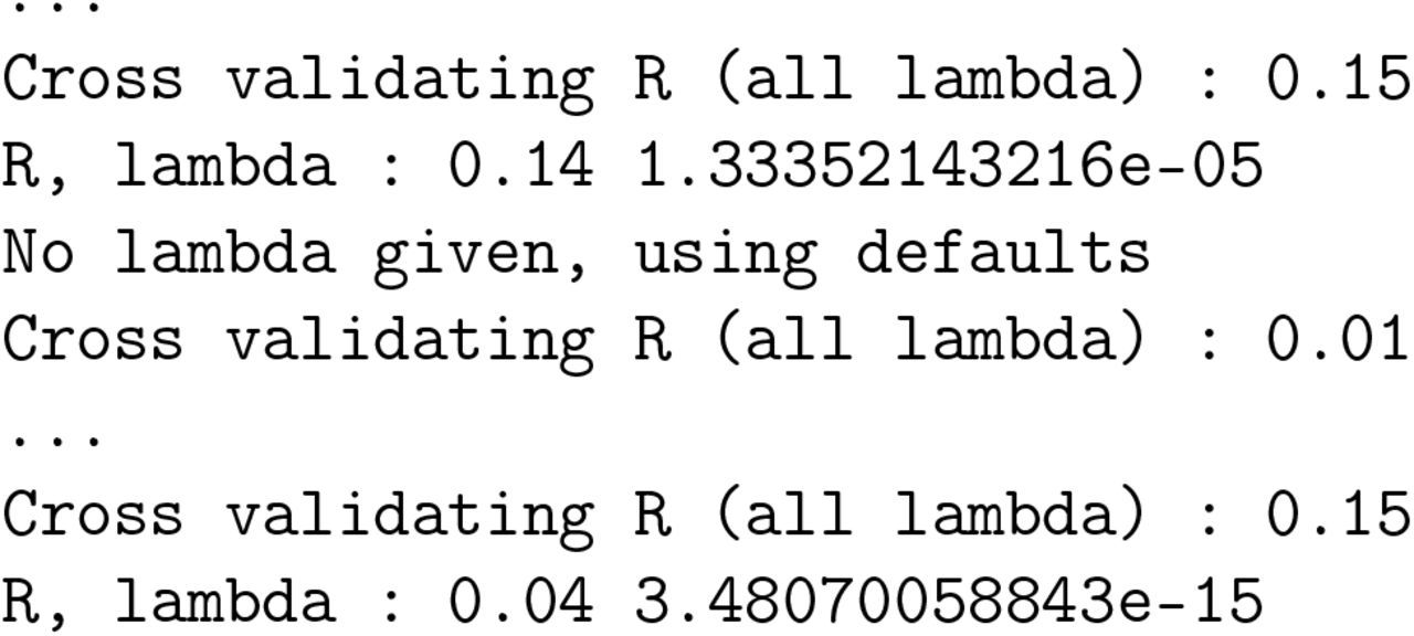
Leave-one-out cross-validation is performed with a single line command. In this procedure we scan a range of R values which set the size of the Gaussian basis functions and the regularization parameter λ values. At the end of this step we obtain the optimal parameters that would correct for overfitting. The function outputs the progress of the cross-validation step and displays the optimal candidates in the last line. Alternatively, one could use the L-curve method to find these optimal parameters. Fig. 11D shows the kCSD reconstruction obtained after cross-validation. We find that this estimation of the current sources resembles the True CSD better.

Noisy electrodes
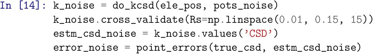
Until now we assumed noise-free data, however, experimental data are always noisy. In this section we investigate how noise affects the kCSD estimation. We first show how to compute the reliability map which we introduced before, Eq. (10). Then we discuss reproducible generation of noisy data with varying noise amplitude. Finally, we study the error in the reconstruction as a function of changing noise level.
Reconstruction quality measure
To assess the estimation quality we measure the point-wise difference between the true sources and the sources reconstructed with the kcsd. We define a function point_errors which takes the true_csd and the estimated_csd as the inputs, normalizes them individually, and computes the Frobenius norm of their difference.

We visualize this difference as before, except we use greyscale colormap to display the intensity of the reconstruction error. For convenience we define the plotting in a function called make_error_plot. The output from this step is shown in Fig. 12A.


Noisy electrodes. A) The error between the True CSD and the estimation obtained with kCSD for a 2 dimensional small Gaussian current source, using the csd seed of 15. The electrodes in this case are assumed to be noise-free. B, C, D) Same as A, however, noise is added to the recorded potentials, whose magnitude is 5%, 10%, or 30%, respectively. E-H) Analogous to A–D, except in this case large Gaussian sources with seed 6 were used.
Noise definition
To study resilience of the reconstruction against the noise in a controlled way we seed the random number generator in the function add_noise. We consider normally distributed noise with the mean and standard deviation set by reference to the recorded potentials.

Source reconstruction from noisy data
With these tools we can study the effects of noise on the reconstruction. We now generate noise for a given noise level between 0 and 100, add it to the simulated potential, and estimate CSD from these noisy potentials. We can then use the error plots to compare the reconstruction with the True CSD. Notice that the parameters giving best reconstruction obtained for noisy data in general will be different from those obtained for clean potentials to compensate for noise.

We can display this error with the make_error_plot plotting function which we defined earlier. Changing the noise_level and the noise_seed affects the reconstruction, but the error depends also on the sources, so changing the True CSD type to a gauss_2d_large or changing csd_seed will lead to different results. This is illustrated in Fig. 12A–D for small Gaussian sources, and Fig. 12E–H for large Gaussian sources, with varying noise levels. The actual ground truth and reconstructions are shown in Fig. 11.
Broken electrodes
It often happens that one needs to discard recordings from a subset of setup. This can happen when some electrodes are used for stimulation and cannot be used for recording, or for data managing purposes the bandwidth limitations may require a compromise between sampling rates and the number of electrodes being monitored simultaneously, or electrode may break down or get too noisy and their signals must be discarded. In this tutorial we discuss how to handle such cases and how to investigate the incurred errors in reconstruction. We first show how we remove recordings from selected (broken) electrodes from considered data. Then we calculate the estimation error for a given source for data from a damaged setup. Finally, we compute the average error across many sources from incomplete data. Note that kCSD reconstruction is designed to work with arbitrary electrode setups. Removing specific electrodes does not change the situation significantly. We focus here on broken electrodes as we see it is a common enough situation in practice that it deserves a consideration. We want to show how one can gain intuition regarding ways and places in which reconstruction may go wrong, when we slightly disturb a setup we are familiar with.
Remove broken electrodes
To test the effects of removed electrodes on reconstruction from a given setup we simulate this with a function remove_electrodes that takes all the electrode positions for this setup and the number of electrodes that are to be removed In this example we remove the electrodes randomly. Like we did previously, to facilitate reproducibility we also pass a broken_seed variable, so that at each subsequent run the same electrodes are discarded. By changing this seed we select a different set of electrodes for removal.

Error in estimation with broken electrodes
After removing the broken electrodes we compute the estimation error to gauge the effect of electrode removal on reconstruction. Here, a fuction calculate_error takes a csd_seed as an input, which selects a specific ground truth source, and all the remaining electrode positions, ele_pos. The function computes the True CSD for a gauss_2d_small type source, computes the potential at these electrode locations, performes kcsd estimation from these data, and computes the error in the estimation of the true csd.

Below (Fig. 13) we plot these errors. We also display the electrodes which were used in the kcsd estimation.

Broken electrodes. A) Shows the average error between the True CSD and the CSD estimated with kcsd for 100 random small Gaussian current sources. B) The same average error as in A, except in this case 5 electrodes were discarded in the estimation. Likewise for C and D, where 10 and 20 electrodes out of the 100 were considered broken. E-H) analogous to A–D, except in this case we show the averages for 100 large Gaussian current sources.
Average error for multiple sources
As we can see, the estimation error depends on the test current sources used. To better understand the effects of the setup we compute the average error across multiple sources. As an example here we show this for two seeds. In principle, any type and number of sources may be tested, as we showed before in analysis of reliability maps. This step is computationally expensive, however, it would normally be carried out only once for a given electrode design configuration. We believe this approach offers useful diagnostics and builds intuition regarding the estimation power for the given setup.

In Fig. 13A–D we show this for the case of 0, 5, 10 and 20 broken electrodes, when the average error for 100 small Gaussian sources was considered. In Fig. 13E–H we show the same for large Gaussian sources.
Discussion
In the present work we returned to the kernel Current Source Density method introduced by [Potworowski et al., 2012] for two reasons. First, to introduce a new Python package for kCSD estimation. In the Results section we provided a brief tutorial to the new package and an overview of its main functions. All the figures in this paper showing CSD and LFP were computed with this package and source files are provided. Second, to discuss some mathematical properties of the kCSD method, especially in view of what information it is possible to extract from sparse sampling of the potential and the limitations of the kCSD procedure. In this section we discuss several issues related to CSD analysis in general and kCSD in particular.
To LFP or to CSD?
Extracellular potentials provide valuable insight about the functioning of the brain. Thanks to recent advances in multielectrode design and growing availability of sophisticated recording probes we can monitor the electric fields in the nervous system at thousands of sites, often simultaneously. One may wonder if this increased resolution makes CSD analysis unnecessary. In our view, as we have discussed many times, it is not so. The long range nature of electric potential means that even a single source contributes to every recording. Thus in principle we should always expect strong correlation between neighboring sites. However, if the separation between the electrodes becomes substantial, on the order of millimeters, the level of correlation between the recordings on different electrodes will decrease. This is because each electrode effectively picks up signals from a different composition of sources. Even if some are shared they are overshadowed by others which may lead to small interelectrode correlations. Still, our experience shows that significant correlations can be observed in the range of several millimeters [Łęski et al., 2007, Hunt et al., 2011] which is consistent with literature [Lindén et al., 2011, Łęski et al., 2013].Fundamentally, the LFP profile is different from CSD profile, and may significantly distort or hide features of importance. For example, Fig. 5.C shows the source composed of three gaussians, while direct inspection of LFP indicates a simple dipole.
In view of these facts we argue that it is always beneficial to attempt kCSD analysis. The caveat is not to believe the reconstructed CSD blindly but always interpret it against known anatomical and physiological knowledge supported by the tools such as provided in the present work (eigensources, reliability maps, etc). In the worst case, for a very small number of electrodes, while the reconstructed CSD will not be a good representation of the true sources, nevertheless, the kCSD procedure will still have the sharpening or deblurring properties and can be thought of as another decomposition method, such as PCA or ICA, simply using physical properties of electric field propagation for signal separation rather than orthogonalization or entropy maximization (or others for other decomposition methods). To use kCSD in this way we would estimate CSD at the positions of the electrodes only since this gives as many values as recorded, does not pretend to introduce new knowledge, but may correct for noise and better localize independent signals. This could be combined with other decomposition methods if desired which may give more physiologically interpretable results [Łęski et al., 2010, Głąbska et al., 2014].
Approaches to CSD estimation
Several procedures for CSD estimation were introduced over the years and are still in use today. The first approach, which probably still dominates today, was introduced by Walter Pitts in 1952 [Pitts, 1952] and gained popularity after Nicholson and Freeman adopted it for laminar recordings [Nicholson and Freeman, 1975]. This was a direct numerical approximation to computation of the second derivative in the Poisson equation (1). Only minor improvements were introduced over the years to stabilize estimation [Rappelsberger et al., 1981] or handle boundaries [Vaknin et al., 1988]. The first major conceptual change was introduced by Pettersen et al. [2006] who introduced model-based estimation of the sources. Their idea was to assume a parametric model of sources, for example, spline interpolated CSD between electrode positions, and using forward modeling to connect measured potentials to model parameters. This model-based approach was generalized by Potworowski et al. [2012] who proposed a non-parametric kernel Current Source Density method which is the focus of the present work.
Apart from these main approaches several variants were proposed. For example, one may interpolate the potential first before applying traditional CSD approach, or the opposite, interpolate traditionally estimated CSD. Although in some cases the obtained results may look close to those obtained with kCSD, we do prefer kernel CSD approach due to the underlying theory which facilitates computation of estimation errors but also yields a unified framework for handling underlying assumptions, noisy data and irregular electrode distributions. In our view approaches combining ad hoc interpolation with numerical derivatives conceptually and computationally are less convincing to iCSD and kCSD and we would not recommend them.
Models of tissue
Throughout this work we assumed purely ohmic character of the sources. This has been debated in recent years [Bédard and Destexhe, 2011, Riera et al., 2012, Gratiy et al., 2017] and it is true that more complex biophysical models of the tissue, taking into account frequency dependent conductivity or diffusion currents, would influence the practice of source reconstruction or its interpretation. However, the available data indicate that in the range of frequencies of physiological interest these effects are small. While one should keep eyes open on the new data as they become available and keep in mind the different possible sources which may affect the reconstruction or interpretation, we believe that the traditional view of ohmic tissue is an adequate basis for typical experimental situations and going beyond that would probably require additional dedicated measurement for the experiment at hand which may not always be feasible. For example, as we discussed in [Ness et al., 2015], the specimen variability of the cortical conductivity in the rat is much bigger than the variability between different directions within a given rat [Goto et al., 2010]. This means that unless we have conductivity measurements for our specific rat we are probably making smaller error assuming isotropic conductivity than taking different values from literature. We feel there is not enough data to justify inclusion of more complex terms in the standard CSD analysis to be applied throughout the brains and species.
In this manuscript we also assumed constant conductivity. We are convinced this is a reasonable approximation for typical depth recordings. In general, however, this approximation needs to be justified or alternative models of tissue need to be considered. In principle, the kCSD method can be applied for a variety of tissue models as long as the basis potentials can be computed from the basis sources while incorporating the geometric and conductivity changes.
For example, Ness et al. [2015] considered a cortical slice placed on a microelectrode array (MEA) in which they included the geometry of the slice and modeled saline-slice interface with changing conductivity in the forward model. They found that Method of Images (MoI) gives a good approximation to the full solution obtained using finite-element model (FEM). This approximation was incorporated within the kCSD method as MoIkCSD variant and is available in the kCSD-python package.
It is possible to generalize kCSD to reconstruct sources from recordings of multiple electrical modalities — LFP, ECoG, EEG. In this case one needs to include the head geometry and the changing tissue properties within the forward model and in the kCSD method. The anisotropic (white matter tracts) and inhomogeneous (varying between skull, cerebro-spinal fluid, gray matter and white matter) electrical conductivity changes can be approximated using data obtained with imaging techniques such as MRI, CT or DTI. Such sophisticated head models require numerical solutions such as finite element modeling (FEM) to compute the basis potentials from the basis sources. We are currently working on this approach to make it generic for any animal head and to eventually utilize it as a source localization method for human data, for example, to localize foci of pharmacologically intractable epilepsy seizures in humans. We call this extension kernel Electrical Source Imaging (kESI).
High density microelectrode recordings
One of the trends clearly observed in modern neurotechnology is the drive towards increasing the number of sensors and their density [Buzsáki, 2004, Berdondini et al., 2005, Frey et al., 2009, Hottowy et al., 2012, Jun et al., 2017, Angotzi et al., 2019], for in vitro and in vivo studies. While it seems that a better resolution for recording spiking activity of multiple cells is the main goal, also more precise stimulation and field potentials monitoring are targeted [Hottowy et al., 2012, Ferrea et al., 2012, Bakkum et al., 2013]. Such massive high density data from thousands of electrodes should greatly increase insight into the studied systems and significantly improve results of CSD reconstructions. There are two obstacles to fully benefit from kCSD analysis of data from these new systems. First, kCSD involves inversion of the kernel matrix which is quadratic in the number of electrodes. Combined with cross-validation the necessary matrix operations quickly become overwhelming. This can be mitigated in a number of ways, by subsampling the data, approximate inversions, and by switching from cross-validation to L-curve method, but the challenge remains. This is the easy problem. The difficult problem is physical. As we move away from a source its contribution to the recorded potential goes down. In consequence, since the present version of kCSD uses all recordings to estimate every source, when using remote signals to estimate local source, we obtain mainly contributions from noise. In effect we get a very reliable estimation of sources varying slowly in space but the sources changing fast in space are treated as noise and silenced by the regularization.
To take full advantage of these data a new approach must be developed. We are currently working on a multiscale approach which we call kCSDHD. The idea is to perform reconstructions in small windows in multiple scales to optimally reconstruct multiscale features of the source distribution and the challenge is to efficiently and correctly stitch them together. This will be reported in the future.
Parameter selection
In the Results section we discussed our strategy for data-based parameter selection using cross-validation or L-curve. Often, we need to tune not just λ but also other parameters. For example, for Gaussian basis sources we may need to decide on the width of the Gaussian used, R. To obtain the optimal set of parameters in that case we compute the curvature of the L-curve or the cross-validation error for some ranges of parameters considered and select parameters corresponding to the maximum curvature / minimum error in the parameter space. This is a simplification of the proposition by Belge et al. [2002] which in practice we found very effective.
As an example, in Fig. 14 we show results of such a scan for the problem shown in Fig. 5. The range of λ to be considered can be set by hand but by default we base it on the eigenvalues of K. The smallest λ is set as the minimum eigenvalue of K which here was around 1e-10. We set maximum λ at standard deviation of the eigenvalues, which here was around 1e-3. The range of R values studied was from the minimum interelectrode distance to half the maximum interelectrode distance. Note that for very inhomogeneous distributions of electrodes this approach may be inadequate.

L-curve curvature (left) and CV-error (right) for the problem studied in Fig. 5. Observe that in both cases there are ranges of promising candidate parameter pairs, R, λ, which can give good reconstruction given the measured data. Red dots shows local extrema for each value of R fixed. See text for discussion of this effect.
What we find is that apart from a global minimum in R, λ space there is a range of R values fixing which we can find optimal λ(R) which leads to very close curvatures / CV-errors / estimation results. What happens is that within some limits we may achieve similar smoothing effects changing either λ or R. Bigger λ means more smoothing, but bigger R means broader basis functions and effectively also smoother reconstruction space. This is why the CV-error and curvature landscapes are relatively flat, or have these marked valleys observed in Fig. 14. This effect supports robustness of the kCSD approach.
The sources of error in kCSD estimation and how to deal with them
Kernel CSD method assumes a set of electrode positions and a corresponding set of recordings. Additionally, single cell kCSD requires morphology of the cell which contributed to the recordings and its position relative to the electrodes. Each of these may be subject to errors.
We assume that the electrode positions are known precisely. This is a justified assumption in case of multishaft silicon probes or integrated CMOS-MEA but not necessarily when multiple laminar probes are placed independently within the brain or for many other scenarios. We do not provide dedicated tools to study the effects of misplaced electrodes on the reconstructed CSD, however, this can be achieved easily with the provided package if needed. The location of the cell with respect to the electrodes is much more questionable, especially in 3D. Nevertheless, the necessary data to perform skCSD are too scarce to start addressing these issues.
On the other hand we do assume that the recordings are noisy and we use regularization to counteract the effects of noise. We have no mechanism to differentiate between electrodes with varying degrees of noise to compensate this differently. However, we observed that for cases with very bad electrodes, similar results are obtained for analysis of complete data and for analysis of partial data with bad electrodes removed from analysis. The difference was in λ selected which was larger when broken electrodes were included in the analysis. Depending on situation, if there is a big difference in the noise visible in different channels, an optimal strategy may be to discard the noisy data and perform reconstruction from the good channels only, which kCSD permits.
The main limitation of the method itself lies in the character of any inverse problem. Here it means that there is an infinite number of possible CSD distributions each consistent with the recorded potential. It is thus necessary to impose conditions which allow unique reconstruction and this is what every variant of CSD method is about. In kCSD this condition is minimization of regularized prediction error. In practical terms one may think of the function space in which we are making the reconstruction. This space is span by the eigensources we discussed before. We feel it is useful to consider both this space as well as its complement, that is the set of CSD functions whose contribution to every potential is zero. This can facilitate understanding of which features of the underlying sources can be recovered and which are inaccessible to the given setup. While for the most common regular setups, such as rectangular or hexagonal MEA grids or multishaft probes, intuitions from Fourier analysis largely carry over, in less regular cases this quickly becomes non-obvious.
To facilitate intuition building in the provided toolbox we include tools to compute the eigensources for a given setup. We also proposed here reliability maps, heuristic tools to build intuition regarding which parts of the reconstructed CSD can be trusted and which seem doubtful. These reliability maps are built around specific test ground truth distributions and some default parameters facilitating validation for any given setup are provided, due to the open source nature of the provided toolbox, more complex analysis is possible if the setup or experimental context require that.
Overview of kCSD-python package
This paper introduces the kCSD-python package — a new implementation of the kernel Current Source Density method [Potworowski et al., 2012] and its two recent variants ([Ness et al., 2015] and [Cserpan et al., 2017]). It is open source and available under the modified BSD License (3-Clause BSD) on GitHub (https://github.com/Neuroinflab/kCSD-python). It has been designed using test driven development and utilizes the continuous integration provided by Travis CI. It supports Python 2.7 and 3.7 versions and has a bare minimal library requirements (numpy, scipy and matplotlib). It can be installed using the Python package installer (pip) or using Anaconda python package environment (conda).
To facilitate uptake of this resource, the package comes with two extensive tutorials implemented in jupyter notebook. These tutorials allow users to test different configurations of current sources and electrodes to see the method in action. These provisions make the advantages and limitations of this method transparent to its users. Furthermore, these tutorials can be accessed without any installation on a web browser via Binder [Project Jupyter et al., 2018]. It is extensively documented (https://kcsd-python.readthedocs.io) and includes all the necessary scripts to generate the figures in this manuscript.
Methods
Review of Kernel Current Source Density estimation
Basis functions
Here we repeat the key steps in the construction of kCSD estimation framework [Potworowski et al., 2012] to introduce the notation and establish the basic notions.
We first construct a pair of related function spaces in which we perform the estimation, space of sources  and space of potentials
  ,
,


We select the basis source functions  so that they are convenient to work with, such as step functions or gaussians, with support over regions which are most natural for the problem at hand. For example, when reconstructing the distribution of current sources along a single cell from a set of recordings with a planar microelectrode array, MC is the neuronal morphology, which we take to be locally 1D set embedded in real 3D space, while MV would be the 2D plane defined by the MEA.
The potential basis functions, bi, are defined as the potential generated by  , so that
  , where :
  . Specific form of
  operator depends on the problem at hand, the dimensionality of space in which estimation is desired, as well as on physical models of the medium, such as tissue conductivity, slice or brain geometry, etc. [Pettersen et al., 2006, Łęski et al., 2007, 2011, Ness et al., 2015, Cserpan et al., 2017]. In the simplest case of infinite, homogeneous and isotropic tissue in 3D we have

In general, we can consider arbitrary conductivity and geometry of the tissue which may force us to use approximate numerical methods, such as finite element schemes. For example, Ness et al. [2015] show an application of kCSD for a slice of finite thickness and specific geometry, as well as a method of images approximation for kCSD for typical slices on multielectrode arrays (recordings far from the boundary, slice much thinner than its planar extent).
In the past we considered CSD reconstruction for recordings from 1D, 2D and 3D setups under assumption of infinite tissue of constant conductivity [Potworowski et al., 2012], we used method of images to improve reconstruction for slices of finite thickness on MEA under medium of different conductivity (ACSF, [Ness et al., 2015]) and we considered reconstruction of sources along single cells when we have reasons to trust the recorded signal to come from a specific cell of known morphology [Cserpan et al., 2017]. All these variants are implemented in the present code. Fig. 1 shows these scenarios.
For laminar probes, Fig. 1.A), following [Pettersen et al., 2006], we assumed elementary current sources contributing to the potential of the form  . Here
  is the one-dimensional basis source (we usually assume a Gaussian of width R). Since information beyond the electrode axis is unavailable we assume rotational symmetry around z. We usually assume H(x, y) a step function on a disk of radius h:

This can be integrated yielding 1D potential basis functions of the form

For planar setups, Fig. 1.B) [Łęski et al., 2011], we usually assume Gaussian basis sources  , physically contributing to the potential with
  , where

This can be integrated to give the potential in the electrode plane:

This approach give two parameters describing the CSD basis functions, the width of the relevant Gaussian, R, and the thickness of contributing layer in 2D case or radius of circular sheath in 1D case (h). Note that if we assume above H(x, y) and H(z) to be Gaussian as well with the same width, in all three dimensionalities the individual contributions are spherically symmetrical Gaussians. Therefore, the same 3D approach can be used. Further, it can be integrated to yield potential in a closed form. Indeed, from eq. (13), taking
 we can show that
 where
where

This is also implemented in the present code.
kCSD framework
We can think of the whole set of the potential basis functions bi(x) as features representing x in a M-dimensional space through related embeddings

Let us introduce a kernel function in  through

This kernel turns  into a reproducing kernel Hilbert space (RKHS, Aronszajn [1950]) whose properties we discussed in Potworowski et al. [2012]. In particular, we can show that all potential profiles admissible by our construction can be written as linear combinations of multiple kernels fixed with one leg at different points:

We introduce the inner product of functions in  ,
, 
 , as
, as

Using this inner product we define the norm in  by
by  , and we induce a norm in
  by
by

Note that we have now two representations of every function in  , as a sum of kernels or a sum of basis elements
 where
where
 where xj are some positions in space.
One can see that in the two representations we have

Source estimation with kCSD
Estimation of current sources with kCSD consists of two steps. The first is kernel interpolation of the potential, the second is changing the space from potential to sources. Conceptually, in the simplest case, this is equivalent to applying Laplacian or double derivative to the potential field obtained in the whole space. However, using our approach with double kernels, which take into account underlying physics and geometry of the studied system, it is possible to apply these ideas to more complex situations, e.g. slices of specific shape and conductivity profile Ness et al. [2015] or fields generated by individual cells Cserpan et al. [2017].
To estimate the potential in the whole space we minimize an error function
 where the first term indicates proximity of our model to actual measurement, while the second constrains complexity of the model2. Using the representer theorem Kimeldorf and Wahba [1971] we can show that the solution is of the form
 where xj are the N electrode positions. Minimum of (23) is obtained for
 where
where

Now that we have the potential given by combination of kernels, Eq. (24), we can expand it in the original basis bi(x), Eq. (20). From that we obtain a consistent estimate of the CSD by lifting the model from the potential to the CSD representation:
 where we introduce the cross-kernel function3

With this definition we can write

Test sources used
In several tests and demonstrations in this paper we use two families of sources which we call small and large sources. They were defined by [Potworowski et al., 2012] in their appendix. They are implemented in functions gauss_2d_small and gauss_2d_large available in file csd_profile.py. Two pdf files with images showing both source families (100 sources each) are available as supplementary materials (large_all.pdf and small_all.pdf). These specific source families were selected to test reconstruction of easy (large) and difficult (small) cases while supporting reproducibility of computations and figures. Otherwise, there is nothing special about them.
Supplementary Materials
Supplementary Fig. 15 shows spectral properties of kCSD method for simple 2D case with 9 regularly distributed electrodes in the square [0, 1] × [0, 1]. This corresponds conceptually to Fig. 2 for the setup from Fig. 7).
Supplementary Fig. 16 shows error propagation maps for 1D regular grid of 12 electrodes. This corresponds conceptually to Fig. 7 for the setup from Fig. 2).
Fig. 17 shows an example of 3D kCSD source reconstruction with the new code. Files small_srcs_3D_all.pdf and large_srcs_3D_all.pdf show 100 examples each of 3D kCSD reconstructions of small and large sources. Similarly, files small_srcs_all.pdf and large_srcs_all.pdf show each 100 examples each of 2D kCSD reconstructions of small and large sources. The files are available at http://bit.ly/kCSD-supplementary.
Fig. 18 shows an example of skCSD reconstruction which corresponds to Fig. 8 from Cserpan et al. [2017]. The simulation, reconstruction and visualization are all reimplemented in Python.

Demonstration of spectral properties of kCSD method for simple 2D case with 9 regularly distributed electrodes in the square [0, 1] × [0, 1] (from Fig. 7). A) Eigenvalues obtained from the decomposition of K for different number of basis sources (M=4, 9, 16, 64, 256), B) Shows the first eigenvalue in the function of growing number of basis, C–K) Shows 9 eigensources (products of  and all the eigenvectors), which combine to produce the inverse solution in kCSD method.

Error propagation maps for 1D regular grid of 12 electrodes (same as in Fig. 2). Every panel represents the CSD contribution (red line) of the potential measured at the corresponding electrode, for which the potential is 1 (green line).

Each column shows five consecutive parallel cuts through a box of size 1. A) Ground truth for the CSD seed of 16. B) Estimated potential; black dots indicate electrodes where potential is colected for further reconstruction. C) 3D kCSD reconstruction from the measured potentials, λ = 0. D) 3D kCSD reconstruction with cross-validation.

Cserpan et al. [2017] of somatic current injection together with random synaptic input patterns for a retinal ganglion cell model. A) Somatic membrane potential. B) Current density and its C) skCSD reconstruction in the segment space. Projection of D) ground truth and E) skCSD reconstruction on the neuron’s morphology at 5 s of the simulation. We simulated a multicompartmental model of a mouse retinal ganglion cell (morphology Kong et al. [2005] obtained from NeuroMorpho.Org Ascoli [2006]) with Hodgkin-Huxley sodium, potassium, and leakage channels in the soma (hh mechanism) in NEURON simulation environment. For calculation of the measured extracellular potentials we used LFPy package Lindén et al. [2013]. The model neuron was stimulated by an injection of oscillatory current to the soma (with frequency of 24.5 1/ms and amplitude of 3.6 nA) together with random synaptic inputs (weight of 0.04 μS) to the dendritic tree. The activity of the model neuron was measured by a rectangular grid of 100 electrodes (10 10, −400 μm 400μm). The figure corresponds to Fig. 8 from [Cserpan et al., 2017].
Acknowledgments
The Python implementation of kCSD was started by Grzegorz Parka during Google Summer of Code project through the International Neuroinformatics Coordinating Facility. Jan Mąka implemented the first Python version of skCSD class. The study received funding from the Polish National Science Centre’s grants (2013/08/W/NZ4/00691) and (2015/17/B/ST7/04123). The authors declare no conflict of interest.
Footnotes
↵† joint first authors
↵1 In the special case when εi are mutually independent and of equal variance σ2, the map of CSD measurement uncertainty can be calculated as a diagonal of
 .
.↵2 Note a typo in eq. (4.2) in the original paper, which incorrectly states the error term as
while it should be , as given here by Eq. 22.↵3 Note that this definition replaces the two variables with respect to the original definition from [Potworowski et al., 2012] to avoid transposition in the matrix formulation below.


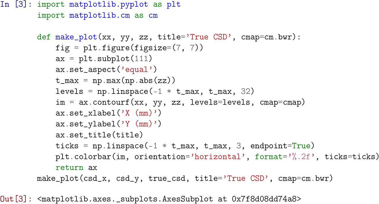
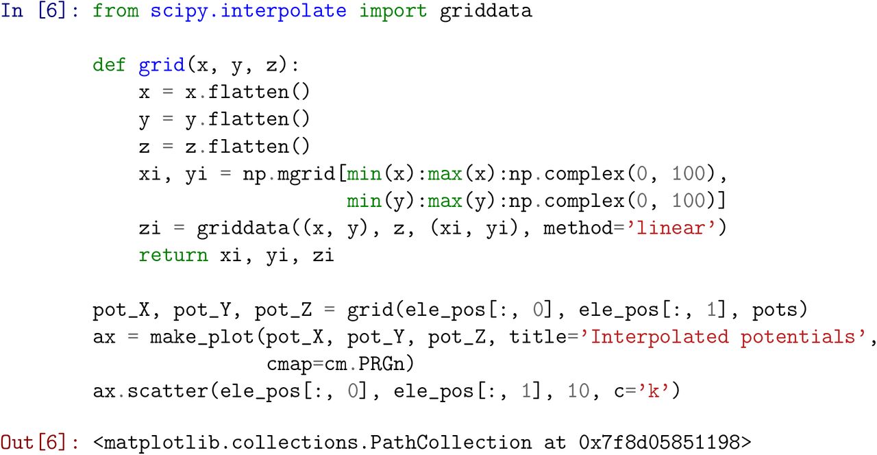
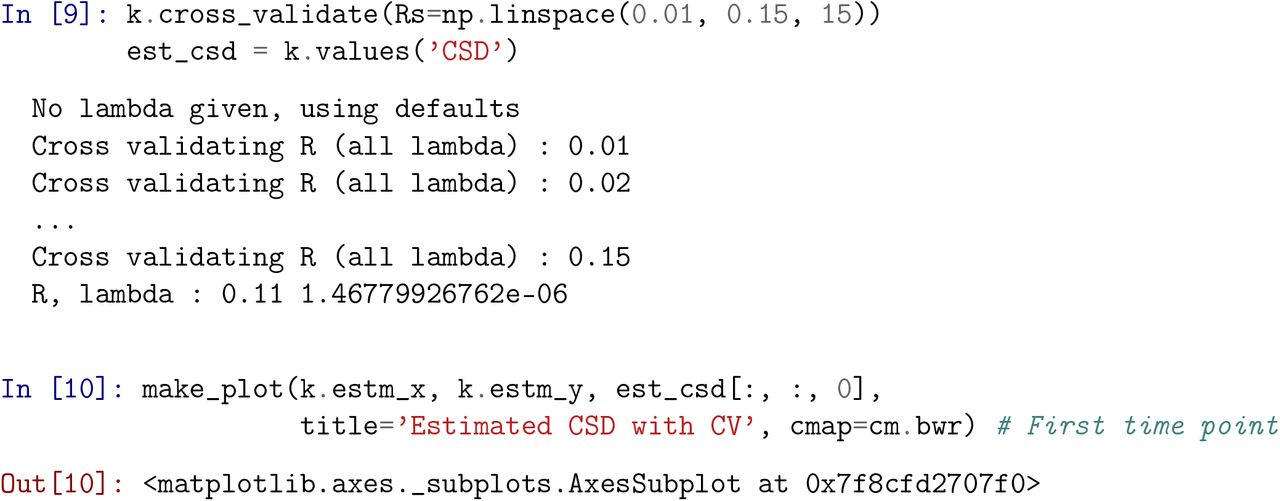
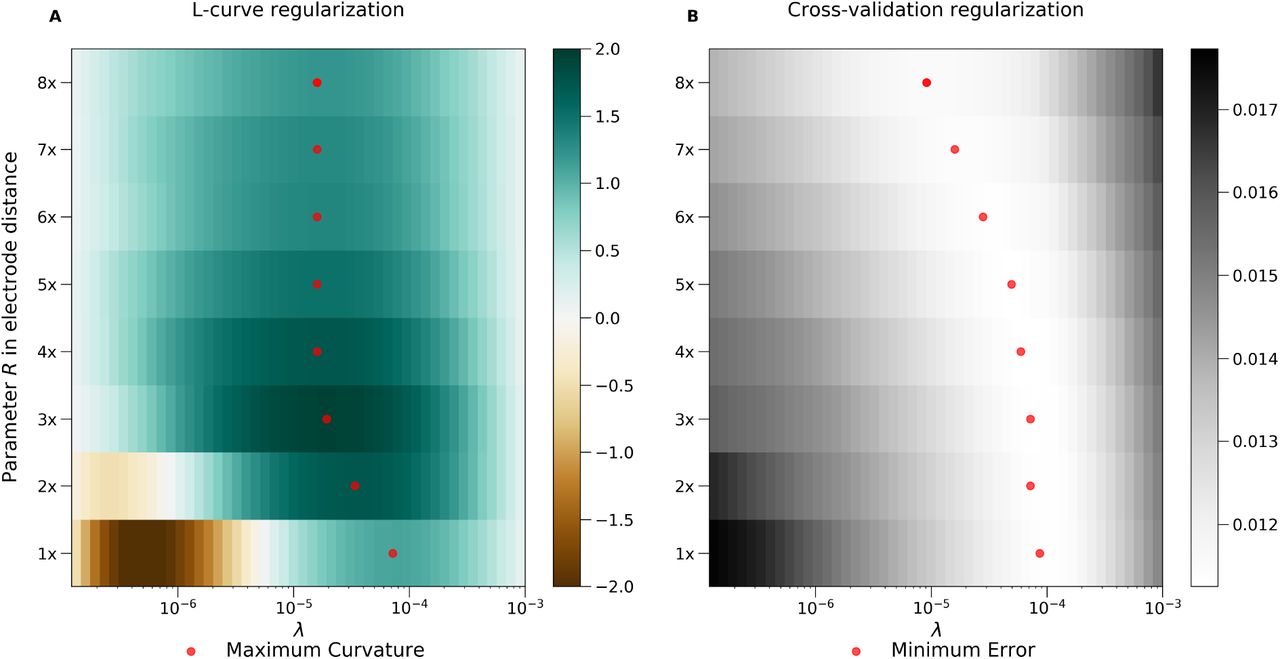
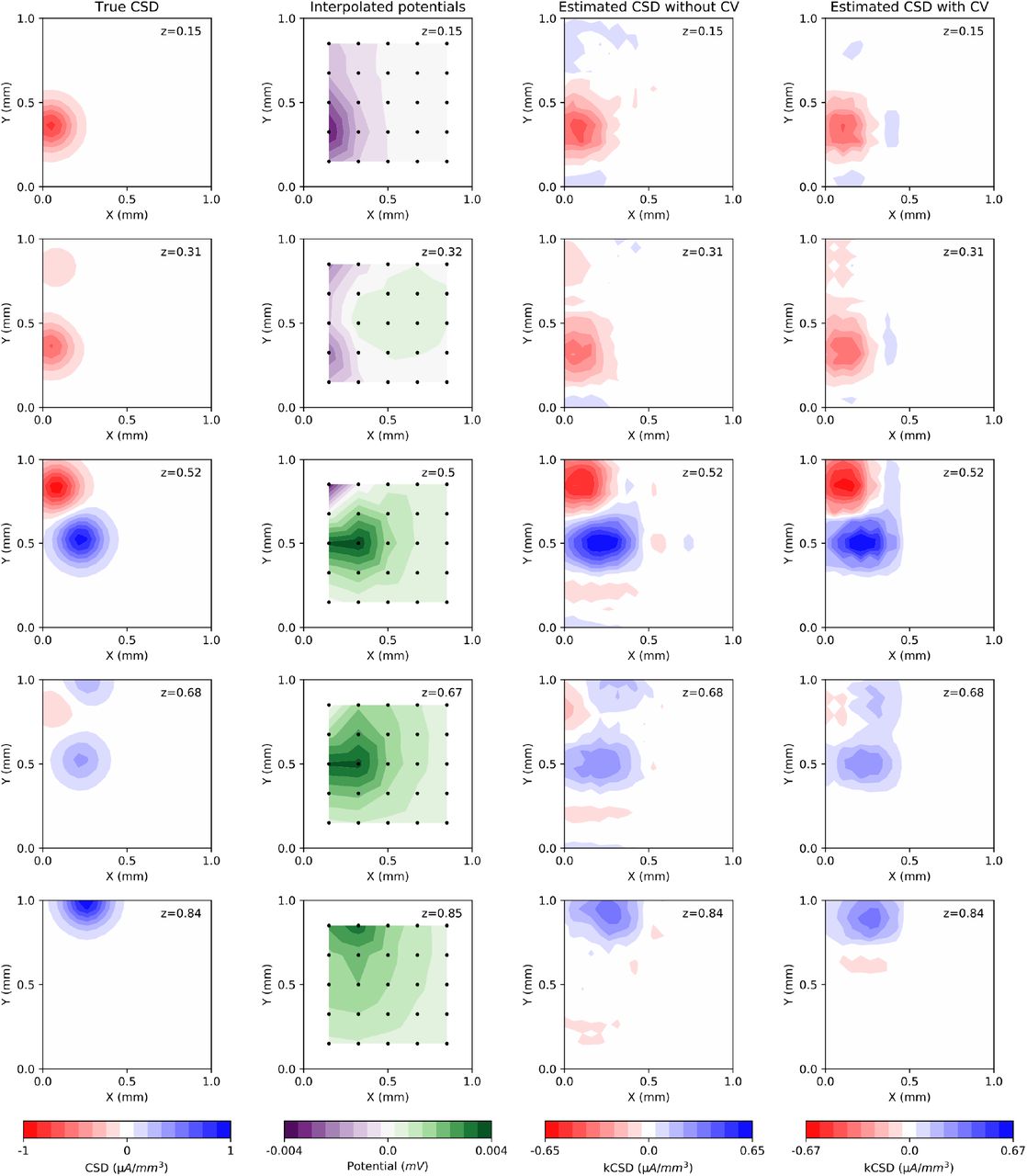