

Abstract
Research in the life sciences has traditionally relied on the analysis of clear morphological phenotypes, which are often revealed using increasingly powerful microscopy techniques analyzed as maximum intensity projections (MIPs). However, as biology turns towards the analysis of more subtle phenotypes, MIPs and qualitative approaches are failing to adequately describe these phenotypes. To address these limitations and quantitatively analyze the 3D spatial relationships of biological structures, we developed a computational method and program ΔSCOPE (Changes in Spatial Cylindrical Coordinate Orientation using PCA Examination). Our approach uses the 3D fluorescent signal distribution within a 3D data set and reorients the fluorescent signal to a relative biological reference structure. This approach enables quantification and statistical analysis of spatial relationships and signal density in 3D multichannel signals that are positioned around a well-defined structure contained in a reference channel. We validated the application of ΔSCOPE by analyzing normal axon and glial cell guidance in the zebrafish forebrain and by quantifying the commissural phenotypes associated with abnormal Slit guidance cue expression in the forebrain. Despite commissural phenotypes that disrupt the reference structure, ΔSCOPE is able to detect subtle, previously uncharacterized, changes in zebrafish forebrain midline crossing axons and glia. This method has been developed as a user-friendly, open source program. We propose that ΔSCOPE is an innovative approach to advancing the state of image quantification in the field of high resolution microscopy, and that the techniques presented here are of broad applications to the life science field.
Introduction
The curious observer
Since Robert Hooke identified cells in a piece of cork, our search for patterns has been informed by qualitative observations. As microscopy and imaging techniques have advanced to generate larger and more complex data, our qualitative abilities are proving to be inadequate to extract all the information these data may hold. The field of biology now faces a problem in which the complexity and granularity of current data collection methods has surpassed the ability of researchers to actually view all of the data collected. Moreover, the subtlety of many of the phenotypes being studied in the modern era, whether slight changes in neuronal positioning in an autism spectrum disease model or the significant perturbations in the size of the brains of children infected with Zika require greater statistical rigor to quantify and detect such phenotypes. In order to overcome these challenges, we need new computational tools to process, quantify, and statistically analyze image based data.
The problems associated with image based data
Analysis of 3D image data is inherently hampered by several obstacles. First, biological specimens present with morphological variation, even from within the same species and age group. Second, all image data contains a subset of positive pixels whose high intensity is due to background noise, which can create ambiguity in isolating the true signal of the sample. Additionally, 3D image data analysis has been most commonly performed on maximum intensity projections (MIPs), which collapses the third dimension of the data in order to present the image in a form that is easier to visualize, and therefore compare. Unfortunately, this compression leads to a loss of information that may be critical to detecting both coarse and subtle phenotypes. Finally, experimental variabilities during image collection further complicate robust characterization of phenotypes. Taken together, the natural biological and experimental variation paired with the data loss of MIP compression, make it challenging to describe meaningful averages of biological phenomena that capture both the unifying features of a sample set and the true sources of variation.
Existing methods for image analysis
Since the emergence of the light microscope, a range of advances in biological imaging have occurred, enabling the acquisition of high resolution data sets of 3D biological structures. These advances however, have intensified the need for more powerful methods to measure changes within and between samples. Currently there are three main classes of image-based analysis: visualization, filter-based analysis and machine learning classification [1]. Tools for visualization have been critical to render 3D-volumetric data; however, 3D visualization tools, such as Amira [2] and Vaa3D [3, 4], rarely extend beyond just rendering the data and lack tools for sample comparisons. Filter-based analysis has been dominated by the open-source program Fiji due to its ease of use and applicability to a wide variety of data types [1, 5]. While Fiji provides a variety of tools and plugins for processing and enhancing features of image data, it also fails to provide rigorous options to compare images between samples. Importantly, machine learning based programs, such as ilastik [6], have excelled at classifying objects and signal within individual images, but unfortunately are unable to classify signals of whole images across an entire sample set. Attempts to overcome some of these challenges have included manually assigning each image a score that corresponds to qualitative assignments of phenotypic variation [7], yet this approach is limited by the error and bias inherent to the human eye. Moreover, such classification approaches are often performed on the whole MIP as opposed to considering the whole image stack, thus rarely discerning subtle changes present in the image.
The biological problem of connecting the two sides of the brain
One such field that has come to rely heavily on image-based data is neuroscience, in particular, research which focuses on uncovering the mysteries of how the central nervous system is built and wired during embryonic development. Visualization of the pattern of developing axon pathways throughout the brain is essential if we are ever to understand how the brain becomes wired and how it might also be repaired to combat neurodegeneration. Commissure development offers a model to study this critical developmental process. The commissure is an important neural structure that serves to connect the two halves of the central nervous systems of bilaterally symmetrical organisms [8, 9]. The commissural tract and the commissures themselves are composed of tightly bundled axons that cross the midline of the organism [7, 9, 10]. Development of these stereotypical structures is initiated by pathfinding axons which, pioneering their way towards the midline in response to local and global signaling cues, which represents a dynamic developmental event with visible degrees of variation [7, 9, 10]. This expected degree of biological variation paired with the additional experimental and image analysis challenges detailed above has hampered the application of robust quantification and statistical approaches to the study of commissure development.
We have taken advantage of the accessible embryonic brain of the zebrafish model system to characterize the first forming commissures during forebrain development [7, 9, 10]. The post-optic commissure (POC) is the first commissure to form, with pioneering axons projecting across the diencephalic midline as early as 23 hours post fertilization (hpf) [11] and is tightly bundled by 30 hpf (Fig 1). Navigation of the first midline crossing axons is mediated by precisely positioned extracellular guidance cues as well as essential cell-cell guidance interactions [7, 8, 12, 13]. This complex array of long- and short range factors function to combinatorially guide pathfinding commissural axons across the midline and onward to their final synaptic target cell.

The post-optic commissure (POC) is formed by midline crossing axons (AT) in concert with a structure of glial cells called the glial bridge (Gfap).
A normal POC is composed of many axons in close association forming a ribbon of axons, or a fascicle [11]. Fasciculation is achieved in part by both the actions of repellent guidance cues limiting the region of allowable space for axon growth and by the positive interactions of axon to axon adhesion. The final shape of the POC resembles a curving band or ribbon of axon fascicles that is 2-3 μms thick at 30hpf as it stretches from one side of the diencephalon to the other. Developing prior to and concomitantly with the POC is a midline spanning swath of glial cells, termed the “glial bridge” [7]. These glial cells are most commonly identified by their expression of the glial specific protein Glial fibrillary acid protein (Gfap), which is an intermediate filament of astroglial cells (Fig 1). These astroglial cells are known to function as both the stem cell of the developing nervous system (also known as radial glia cells) and as a supportive cellular substrate for migrating cells and pathfinding axons [7, 9–11, 14].
In order to study the development and relationship between the POC and the glial bridge, we have employed immunocytochemistry (ICC) to label the two structures using antibodies against acetylated tubulin (anti-AT, axons) and Gfap (anti-Gfap, astroglia) (Fig 1). Imaging with confocal microscopy enables us to collect high resolution 3D data sets of the labeled structures within the zebrafish forebrain. Our analysis of these imaged structures has been limited due to the variable nature of its biology as well as inconsistencies inherent in the methodology. Further complicating this analysis is the amorphous distribution of Gfap labeling, which defies confidence in any qualitative inspection. To overcome these challenges we have created a new computational method we call ΔSCOPE (Spatial Cylindrical Coordinate Orientation with PCA Examination). This method aligns the gross morphology of each biological sample in 3D space before assigning a new set of relational coordinates, which serves to directly represent the biological data contained within an image relative to a model of the imaged structure, consequently enabling statistical comparisons to be performed. We validate the use of ΔSCOPE as a tool to quantify biological structures by quantitatively describing the relationship of POC axons and glial bridge cells during commissure formation, and quantifying differences between wild type commissures and mutants lacking normal axon guidance cue expression. We conclude that ΔSCOPE provides a novel approach for the quantification of biological structures that we propose will be of broad application across the life sciences.
Results
Development of ΔSCOPE – analysis of biological structures
This study is motivated by our interest in understanding how different cell types interact during commissure formation in the vertebrate brain, which is a broad objective that required the development of a new 3D-imaging program capable of comparing commissures from different sample types. Moreover, for such a computational method to be effective, it needs to address four major challenges that we have identified which limit image analysis: image noise, experimental variation due to biological and sample based misalignment, loss of sample dimensionality, and a lack of statistical power when comparing between images.
Our approach to developing a new 3D image analysis program was to register the data around the presence of a common biological structure onto which all of the analysis can be anchored. To study the development of neuronal wiring, we focused on the formation of the POC during embryonic forebrain development. The POC is structurally composed of bundled axons derived in part from neurons of the ventral rostral cluster in the diencephalon [9, 11, 15, 16]. POC axons can be made experimentally visible with immunocytochemical procedures using antibodies that recognize Acetylated Tubulin (AT), which establishes the primary structural channel for our analysis. Any secondary structural markers, such as anti-Gfap for astroglial cells, will always be registered and processed relative to the primary structural channel (the POC in our case). We present ΔSCOPE as a program that 1) takes in confocal image stacks of the POC and secondary structures 2) outputs quantitative comparisons between sample types of both primary and secondary structures, and 3) quantifies and identifies statistically significant biological differences and distributions between the primary and secondary structures within a sample set (Fig 2).

In a clockwise manner, ΔSCOPE processing involves: 1) collecting and immunostaining samples 2) generating confocal stacks of immunostaind samples with close to isotropic voxels 3) processing confocal stacks with ilastik 4) performing principal component analysis in the resultant data 5) changing the coordinate system of the data to be biologically appropriate 6) calculating bin sizes and then binning signal into landmarks 7) performing statistical tests.
Before ΔSCOPE analysis can be performed, image pre-processing is necessary to isolate true structural signal from experimental and biological noise contained in the image. To reduce the potential negative impacts associated with a poor signal-to-noise ratio acquired during image acquisition, we took advantage of the existing interactive machine learning program, ilastik, which relies on user input to create a training dataset consisting of images labeled for signal and background [6]. ilastik distinguishes signal from noise by generating a probability value ranging from 0 to 1 for each pixel indicating the probability that it is true signal (Fig 3 A). We applied a 0.5 probability cutoff to select a set of points representative of true signal for each channel. This probability-based threshold enabled confident selection of points that relied on statistical significance as opposed to intensity thresholds (which can exclude real signal in fainter images). To ensure the data in each sample set was equally represented and pre-processing results were not skewed by overly faint or bright data points, a new ilastik training file was generated for each channel within each sample type. Thus, the AT channel in wild type samples was processed separately from the AT channel of mutant samples.
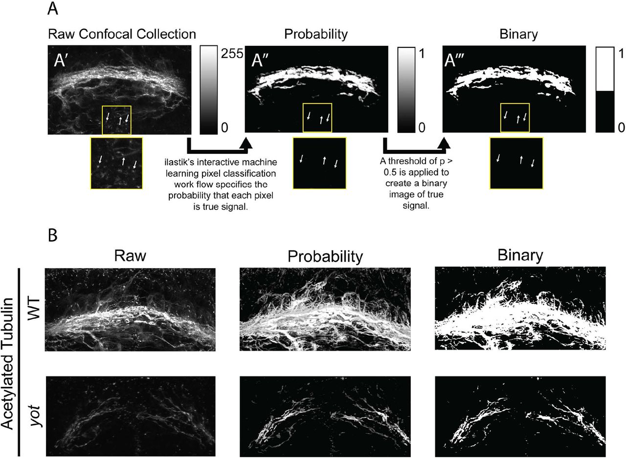
(A) ilastik’s machine learning pixel classification work flow enables the selection of a binary set of points that represent true signal after eliminating noise and variable intensity. (B) ilastik’s machine learning processes images to reduce contamination of secondary signal from cilia while retaining axonal labeling.
ilastik pre-processing helped to overcome the challenge of differential intensity that can arise from photo-bleaching, poor, or differential labeling in samples. Additionally, ilastik offered the capability for trained machine learning, capable of removing spurious signal from contaminants and secondary sources of noise throughout the z-stack. Importantly, antibodies against AT are known to label not only axons but cilia as well, such as the prominent primary cilia found lining the cells of the ventricles throughout the brain [17]. Our training of ilastik successfully reduced the impact of the secondary labeling of the ciliary structures found in our samples while preferential optimizing the identification of true axon signal (Fig 3).
Principal component analysis aligns samples on biological axes
For any comparison of biological samples to be possible, the structures being analyzed must be consistently oriented in 3D space. Uniform alignment of samples enables direct measurement of differences between samples. However, the position and shape of biological structures, like the POC, are variable due to natural variation in biological samples, and due to inconsistencies in experimental preparations, specimen mounting procedures, or microscopic acquisition protocols. These inconsistencies lead to individual differences in how the samples are oriented in 3D space, and presents significant barriers for accurate sample to sample alignment, and consequently, problematic statistical comparisons between experiments.
To compensate for variation in sample position, we applied principal component analysis (PCA), which enables the isolation of a consistent, unbiased set of biologically meaningful axes from anisotropic 3D biological samples - where each dimension is proportionally different in size. The use of PCA in ΔSCOPE relies on the primary structural channel to calculate the PCA transformation matrix, which in our study is the axon labeled channel (anti-acetylated tubulin). Any secondary channels such as astroglia (anti-Gfap) are similarly transformed according to the matrix calculated for the structural channel.
The position of each point in the ilastik-generated binary dataset of true signal is scaled by the dimensions (μm) of the voxel. In order to prevent fine structures, such as wandering axons, from interfering with the core morphology of the commissure (and primary structural channel), we apply a median filter twice to smooth the structure and remove fine processes (Fig 4 A). PCA identifies the orthogonal set of axes in the dataset that capture the widest range of variability in the data (Fig 4 B); therefore, the median filtering we applied serves to smooth out outlier signal and convolve individual fascicles into a singular structure. Selection of median filter size is dependent on the thickness of the structural signal, and thus requires adjustment to best suit the sample set.

(A)Axons of the POC tend to wander and deviate from the central core of the commissure. While axons preserved in the probability MIP on the left are biologically relevant, they can interfere with the alignment process. On the right, duplicate application of a median filter to the axon data extracts the core structure of the commissure while eliminating fine processes that could interfere with alignment. (B) PCA is applied to n-dimensional data to identify axes that capture the most variability in the data. 1) In this two dimensional example, the first principle component (PC) is identified and the second PC is oriented perpendicular to the first. 2) The data is rotated so that the first PC is horizontal and the second PC is vertical. 3) Finally, the data is shifted so that the center of the data is at the origin. (C) After applying PCA to a single POC sample, the arc of the commissure lies in the new XZ plane with the midline positioned at the origin. In each 2D projection, the intensity of each point corresponds to depth in the third dimension.
Since biological structures frequently maintain consistent proportions, PCA can use the median filtered data to isolate three orthogonal axes that are consistent between samples (Fig 4 C). Importantly, we only used the median filtered data to align channels but did not use it for data analysis. After PCA, each image is visually inspected to ensure that the structure is appropriately fit to each axis. ΔSCOPE comes complete with a set of alignment tools to make informed corrections to the PCA alignment.
The relative X-axis of our images of the POC consistently spans the medial-lateral dimension of the embryo and consequently contains more variability than the other dimensions, therefore PCA identifies the X-axis as the first principle component (Fig 4 C). For samples in which most of the signal in the X-axis is lost however, errors PCA axis assignment can result, which can be overcome by manually assigning the X-axis as the first PCA component. Additionally, the anatomical dorsal to ventral axis of the forebrain commissures at the embryonic stages examined are collected in the relative Z-axis, which typically has a greater range of values as compared to the anatomical anterior to posterior axis that is assigned to the Y-axis, however, this is not definitive, and does not affect PCA axis assignment.

In order to ensure that all samples are in the same position following the alignment process, we then fit a polynomial model to the data and identify a centerpoint for translation to the origin. We mathematically described the shape of the POC with a parabola, such that the vertex of the parabola signifies both the center of the data and the position of the origin. Following PCA alignment, the commissure lies entirely in the XZ plane with the midline of the commissure positioned at the origin (Fig 4 C). The same transformation and translation completed on the structural channel was then applied to the secondary channel.
Cylindrical coordinates define signal position
Following PCA alignment, each point is still described by x, y, and z Cartesian coordinates; however, these coordinates are not directly related to the structure itself and thus limited in their applicability to the analysis of the structure in question. In order to facilitate direct comparison of specific structures in 3-dimensional space, we implemented a cylindrical coordinate system that is defined relative to the biological components of the structure itself. To calculate these new coordinates, we assume that the structure, specifically the POC, has an underlying shape that is consistent between samples and can be described by a parabola fit to anti-AT labeling.
We next defined a set of relative cylindrical coordinates that are oriented around a single axis in 3D space, which in our case is the POC parabola. Each point in the data is assigned three new values that describe its position relative to the parabola as the central axis: distance from the model (R), angular position around the model (θ), and distance from the midline along the model (α) (Fig 5). These new coordinates serve as parameters that contain biologically meaningful information about the shape and composition of the structure. α describes the position of points relative to the midline or periphery of the commissure. Depending on the embryonic stage being analyzed, θ captures the dorsal-ventral or anterior-posterior position of the point. Finally, R describes how far a point is from the commissure, which is informative to the degree of axon fasciculation observed in the commissure or the distribution of secondary channel around the commissure.

Creating a cylindrical coordinate system around the POC. To enable analysis of data points relative to a biological structure, points are transformed from a Cartesian coordinate system (x, y, z) into a cylindrical coordinate system (α,θ,R) defined relative to the structure of the commissure. This new coordinate system provides biologically relevant metrics of position.
Building Landmarks to compare samples
The conversion of our image data into cylindrical coordinates enabled each point to encode biological information relevant to the development of the POC. We next binned the data by establishing regularly spaced landmarks – a method of analysis commonly used in morphological studies, which would enable statistical test and comparison between similarly positioned bins [18]. Typically, landmarks are assigned to distinct locations or points on a shape of interest, which are used for direct comparison between samples and quantification of any differences that may exist between those samples. Although historically landmarks were often assigned by an expert with domain knowledge of the structure, we took an approach that eliminated possible human biases by mathematically calculating a set of landmarks which were regularly distributed across the structure.
To calculate a set of landmarks across the POC, we divided the commissure into a set of bins in the α and θ axes (Fig 2). Within each α θ bin, two representative metrics are calculated to describe the nature of the signal: 1) the median R distance of the signal and 2) the total number of points of signal. The θ dimension is divided into 8 evenly spaced bins, each of π/4 radians in order to enable visualization of signal around the commissure. This division enables resolution along biological axes (anterior-posterior and dorsal-ventral) without oversampling. The number of bins along the α dimension was set to include and bin together several microns in each bin.
This array of landmarks can be used identify regions of the commissure that may differ between sample sets. In order to test the statistical significance of landmark differences between sample sets, a t-test is performed comparing the median R values of a landmark in one sample set to another. Tests are performed only between the same structural points between sample sets, and significance is set at a p-value of 0.01. These parameters resulted in 88 total tests performed in each set of structural comparisons. Since each landmark test is not comparable to each adjacent test and the number of samples being tested is less than the number of landmarks being calculated, multiple testing solutions were found inadequate for these purposes. Therefore, we examined regions of significant change that were defined as exhibiting differences in a minimum of 3 adjacent landmarks with statistical significance at a level of p<0.01.

Calculation of biological landmarks. In order to facilitate direct comparisons between samples, we subdivide the data into a set of representative landmarks. 1) The POC is divided into equal slabs along α. 2) Each α slab is divided into 8 θ wedges of 45°. 3) The set of points in each wedge consists of a set of R values that can be visualized in a histogram. In order to reduce a set of points to one representative point, we calculate the median R values in the wedge. 4) Each landmark point can be plotted and visualized according to the average α and θ values for the wedge and the median of the R values in the wedge
Interpreting ΔSCOPE landmark results
ΔSCOPE is designed to leverage biological replicates,in order to reduce overall biological noise and thus amplify significant shifts and changes in signal morphology. The position and density of the post-optic commissure is defined by the pathfinding fidelity and quantity of axons spanning the diencephalon. Our interpretations of ΔSCOPE analysis is based on two key assumptions. 1) the more axons present within a set landmark wedge, the higher the positive pixel count at that landmark will be. 2) A highly fasciculated commissure (axons all tightly bound to one another) will be represented by lower radial distance values at the midline, which will be represented by more pixels being found in proximity to the POC parabola. Using these metrics we have evaluated the utility of ΔSCOPE as a new methodology for image quantification to examine commissure development over time, as well as for the analysis of both gross and subtle structural differences.
Validation of ΔSCOPE through analysis of known mutant phenotypes
We approached the validation of ΔSCOPE by analyzing several different degrees of commissure manipulation from a severe loss of midline axon crossing to more subtle axon and astroglial cell mispositioning. Finally, we then confirmed that ΔSCOPE analysis appropriately matched the degree and presentation of commissural defects in published commissural mutants.
To validate the efficacy of ΔSCOPE analysis and quantification, we first tested its accuracy in quantitatively describing the severe POC and glial bridge defects reported in the you-too (gli2-DR; yot) mutant [7]. Homozygous yot mutants express a dominant repressive form of the Gli2 transcription factor, which functions to repress the Hedgehog signaling pathway in those cells normally expressing the gli2 gene [19]. We have previously shown that loss of Hedgehog signaling in the yot mutant causes the misexpression of the Slit family of guidance molecules that play essential roles in directing POC axons across the diencephalic midline of the zebrafish forebrain. More specifically, yot mutants exhibit expanded expression of slit2 and slit3 throughout midline regions where they are normally absent. In contrast, slit1a was found to be reduced in the forebrain of yot mutants compared to controls [7]. Slit2 and Slit3 are accepted to function as axon guidance repellents, thus their expanded expression is hypothesized to be responsible for the reduced midline crossing seen in yot mutants [7]. The function of Slit1a is currently unresolved. The consensus on the qualitative severity of POC loss in the yot mutant provides our study here the best reference phenotype to validate the utility of ΔSCOPE to accurately describe this POC defect. Moreover, we sought to analyze both axon and glial cell development during POC formation in yot mutants with ΔSCOPE not only for its validation, but to provide the first quantitative assessment of yot commissural phenotypes.
We first tested the ability of ΔSCOPE to detect significant reductions in the amount of POC axon (anti-AT) signal present at the diencephalic midline of yot mutants and wild type siblings as a measure of midline crossing. The secondary labeling of cilia by the anti-AT antibody posed an initial challenge for analysis particularly in yot mutants that lack a majority of the primary axonal labeling at the midline (Fig 9). This extraneous anti-AT signal is especially apparent in the forebrain ventricles, which can artificially contaminate the true signal for the structural axon channel. Moreover, yot mutants also display more non-commissural AT labeling deeper into the forebrain that can also obscure POC-specific midline crossing axonal labeling. Therefore, we first attempted to train the machine learning preprocessing of ilastik to reduce the influence of the ciliary tubulin or deeper axon labeling.

The you-too mutant (gli2-DR) experiences a loss of commissure formation (AT) (Green) as compared to WT and disruption to the glial bridge (Gfap) (Red).
We show that applying ilastik’s pixel classification algorithm as part of the ΔSCOPE methodology does effectively reduce ciliary labeling and significantly reduced contributions from signal derived from non-commissural axons (Fig 8). Visual observation of MIP’s from pre- and post-processed wild type and you-too embryos shows that ilastik processing greatly reduced cilia labeling and reduced extraneous labeling of axons around the commissure. This pre-processing has successfully isolated the real commissural signal within the full 3D data sets and prepared it for the next steps in ΔSCOPE analysis, that of PCA and landmark calculations.

Raw collections from the confocal microscope are processed by ilastik following training based on 5-10 representative samples. The resulting probability images contain the probability that each pixel is signal or background. Finally a threshold is applied to the probability image in order to extract a set of binary points. Following ilastik processing, faint axons are enhanced and preserved while points of ciliary labeling are eliminated. Faint Gfap signal is greatly enhanced in both wild type and mutant samples.
PCA pre-processing for wild type samples was conducted with a median filter of 20 pixels, which was determined to be sufficient to enable PCA alignment. However, when we applied a median filter of 20 pixels to yot mutant samples it resulted in a loss of most of the data at the midline. This reduced labeling was due to the know reduction of midline crossing of axons, and was therefore a feature we desired to capture in our statistics. We empirically determined that a median filter of 10 pixels was sufficient to reduce noise while still enabling alignment of the sparse axonal commissures seen in the yot mutant.
ΔSCOPE analysis of POC axons in you-too mutants
PCA aligned samples were then assigned landmarks using the protocol previously described above. The results of landmark analysis of wild type and yot mutant axons are graphically represented and depict regions of two opposing wedges of landmarks (Fig 9). To quantify whether POC axons were significantly mispositioned in yot mutants, we analyzed the defasciculation metric (the median radial distance (R)) of axons from the modeled POC parabola. Our analysis revealed significant increases in the radial distance of signal in homozygous yot mutants at the midline and along the whole tract of the commissure as compared to homozygous wild type siblings (Fig 9). More specifically, we observed that signal lies between 3-5 μm from the calculated model in all radial axes of wild type commissures (Fig 9), light green line, top panel). In contrast, anti-AT signal in yot mutants ranged in distance from 5 to 15 μm from the modeled POC parabola, with the greatest deviations observed at the midline (Fig 9), dark green line, top panel). Furthermore, the greatest magnitude of difference was observed along the ventral anterior (Fig 9 A) and dorsal anterior axes (Fig 9 C,D). The average distance of anti-AT signal in yot mutants from the midline was 15 μm as compared to the tighter fasciculated wild type commissure (wt, R = 3 μm). Little divergence was observed along the posterior axes dimensions (dorsal-posterior (Fig 9 A,B):WT R = 2 μm; yot R = 8 μm; ventral-posterior (Fig 9 C,D); WT R = 2 μm; yot R = 14 μm). Biologically, these data suggests that commissural axons in yot mutants are distributed more dorso-ventrally (towards the pre-optic area or yolk salk respectively) and that wandering axons in yot are preferentially located more superficially near the epithelium of the forebrain as opposed to pathfinding deeper into the forebrain.

Analysis of changes in amount of axon signal (A-D) and distance of axon signal from POC model (E-H) in WT (n=37) and yot (n=33) 28 hpf embryos. Top of data plots correspond to the top half of the corresponding radial plot, and bottom to the bottom. Significant differences p¡ .01 are denoted by black filled circles. A-D) Significant increases in the radial distance of axon signal are observed in all α and R positions in yot embryos. We observed an increase in average R distance of 3-5 μm in wild type embryos to 5-15 μm in yot embryos. E-G) Significant reductions in At signal are observed in the dorsal posterior axis at the midline. F-H) Significant reductions in the ventral-posterior axis are observed in yot embryos.
To confirm that fewer POC axons were crossing the midline in yot mutants as previously described in Barresi et al. 2005 [7], we used ΔSCOPE to quantify the number of anti-AT pixels at and around the midline. We observed significant reductions in positive pixel number at the midline in yot mutants, which were most pronounced along the dorsal and dorsal-posterior axes (Fig 9 E-G). ΔSCOPE also detected significant but intermittent reductions in the number of anti-AT pixels (axons) in the ventral and ventral-posterior axes along the commissures’ periphery (Fig 9 F-H). Reductions in the amount of signal in the periphery of yot mutants could be due to fewer axons projecting towards the midline (ispilateral side) and/or fewer axons extending away from the midline following crossing (contralateral side).
ΔSCOPE analysis of the glial bridge in you-too mutants
The fibrous and compositionally amorphous pattern of anti-Gfap, a label of astroglial cells in the zebrafish forebrain, has made any robust quantitative characterization of their positioning difficult and substantially inadequate to date. Prior attempts to qualitatively describe diencephalic glial bridge have suggested that the glial bridge was spread out along the dorsal/anterior to ventral/posterior dimensions in yot mutants [7]. Continuing to use the modeled POC parabola as a structural anchor for sample comparisons, we applied ΔSCOPE to the analysis to the secondary anti-Gfap channel to uncover whether the more obscure phenotypes in the glial bridge can be detected and quantified. yot mutant embryos exhibited sporadic Gfap signal closer to the POC model than that seen in wild type embryos. Interestingly, we find that these reductions in the distance of Gfap signal from the POC model were found in both the ventral and dorsal posterior axes (Fig 10 A-D). Concomitantly, we also observed reductions in the amount of Gfap signal detected in yot mutants along these same posterior axes, with the most significant reductions found in the commissure periphery (Fig 10 E-G). Intriguingly, these same posterior axes correlate with the locations also lacking significant anti-AT (axon) signal in both WT and yot mutant commissures (Fig 9). These data taken together suggest that in yot mutants, Gfap+ astroglial cells or cell processes are reduced in the same locations where commissural axons are normally found in wild type embryos, namely the dorsal posterior axes (compare (Fig 9 A,B with (Fig 10 A,B) as well as in the periphery of the ventral-posterior axes (compare (Fig 9 G,H with (Fig 10 G,H). No significant reductions were observed in Gfap signal along the anterior axes. We note that both the amount and positioning of Gfap signal was not significantly different in anterior or anterior ventral positions (Fig 12 A, B, D-F, H). We interpret this data, when combined with the lack of posterior signal underneath the commissure, to suggest that it results in the apparent redistribution of the remainder of the Gfap signal laying in the ventral axis.

Analysis of changes in amount of Gfap signal (A-D) and distance of Gfap signal from POC model (E-H) in WT (n=37) and yot (n=33) 28 hpf embryos. Top of data plots correspond to the top half of the corresponding radial plot, and bottom to the bottom. Significant differences p¡ .01 are denoted by black filled circles. A-D) Significant reductions in the radial distance of Gfap signal are observed in midline dorsal posterior α and R positions bins in yot embryos. We observed an reduction in average R distance from 10-25 μm in wild type embryos to 10-20 μm in yot embryos. E-H) Significant reductions in Gfap signal are observed in the dorsal posterior axis at the midline in yot embryos.
Quantification of the development of the POC
Demonstration of ΔSCOPE to successfully quantify both axon and glial phenotypes in the yot mutant led us to next ask whether ΔSCOPE can also quantitatively describe how axon-glial interactions change over the course of commissure development. In the zebrafish, 22 hpf is the earliest embryonic time point when sufficient commissural axon signal (anti-AT) is visible, and thus prevents the usage of this primary structural channel for ΔSCOPE application to any stages prior to 22 hpf. Therefore we examined and analyzed POC and glial bridge development specifically between 22 and 30 hpf which captures both the pioneering midline crossing events as well as the thickening of the POC.
We performed immunocytochemistry on embryos fixed every two hours from 22 to 30 hpf using antibodies that recognize AT and Gfap. For each time point, we quantified the number of positive pixels and radius from the modeled POC parabola. We used a students t-test to compare adjacent time points, such as 22 hpf to 24 hpf and 28 hpf to 30 hpf. Between 22 and 30 hpf, we observed significant increases in the number of positive pixels of anti-AT signal at the midline, which is indicative of progressive axon fasciculation over time (Fig 11). Interestingly, the largest increases in anti-AT signal occurred between 24 and 26 hpf (Fig 11 E-H), which was also paired with significant reductions in the distance of signal from the modeled POC parabola in all radial axes (Fig 12 E-L). This comprehensive axonal condensation around the modeled POC parabola was preceded by an earlier statistically significant reduction in the radial distance of the anti-AT signal along the dorsal-anterior axis between 22 and 24 hpf (Fig 12 B-D). Importantly, during this same early time period (22-24 hpf) the amount of axon signal did not change; however, by 26 hpf asymmetric increases in anti-AT signal were quantified along the anterior-posterior axes (Fig 11 E-H). We interpret the biological relevance of these data to suggest that the early reductions in median R distance with no corresponding change to the number of points represents axons undergoing a period of error correction as they pathfind across the midline. However, soon after this first period of midline crossing, the number of points increases as median R distance continues to decrease, which defines the period of mounting commissural fasciculation. This interpretation is further reinforced by the absence of a detection of an increase in radial distance, despite increases in the amount of axon signal.

A-D) Statistical comparison of the number of positive pixels in 22 hpf (n=13) and 24 hpf (n=20) POCs’. No statistical differences are observed. E-H) Statistical comparison of axon positive pixels between 24 hpf (n=20) and 26 hpf (n=18). Significant changes observed in anterior ventral positions. I-L) Statistical comparison of axon positive pixels between 26 hpf (n=18) to 28 hpf (n=17) POCs’. No statistical significance observed. M-P) Statistical comparison of axon positive pixels between 28 hpf (n=17) and 30 hpf (n=17). Significant changes observed in anterior positions only.

A-D) Statistical comparison of the radial distance of axon signal from the POC model in 22 hpf (n=13) and 24 hpf (n=20) POCs’. Statistical reduction in radial distance was observed in anterior positions. E-H) Statistical comparison of the radial distance of axon signal from the POC model in 24 hpf (n=20) and 26 hpf (n=18). Significant reductions in radial distance was observed in all positions. I-L) Statistical comparison of the radial distance of axon signal from the POC model in 26 hpf (n=18) to 28 hpf (n=17) POCs’. No statistical significance observed. M-P) Statistical comparison of the radial distance of axon signal from the POC model in 28 hpf (n=17) and 30 hpf (n=17). No significant changes observed.
Quantification of glial bridge development
Having quantitatively described the development of POC axons during commissure formation, we next sought to determine how the cells of the glial bridge may be changing relative to the assembly of the POC. Using the modeled POC parabola as the primary structural channel, we applied ΔSCOPE to the Gfap labeling of the secondary channel. This analysis detected the earliest positional changes in astroglial cells to a focal reduction in the radial distance along the dorsal-anterior axis between 22 hpf and 24 hpf (Fig 13 D). Moreover, by 26 hpf significant reductions in Gfap radial distance moved to an expanded area associated with both the posterior and ventral-posterior radial bins (Fig 13 E-H). Importantly, no positional changes in Gfap labeling were quantified after 26 hpf (Fig 13 I-P); however, the amount of Gfap signal was determined to significantly increase during this time. After a modest but statistically significant reduction in Gfap signal between 22-24 hpf along the ventral axis, glial bridge labeling was first seen to increase at the midline specifically along the anterior axis between 24 and 26 hpf (Fig 14 E,H). Interestingly, between 26 and 28 hpf the amount of Gfap signal continued to increase, but now along the dorsal-ventral axis of the midline and separately in the posterior periphery of the commissure (Fig 14 I-L). Surprisingly, after this central peak of increases in Gfap signal between 24 and 28 hpf, by 30 hpf the glial bridge appears to show a targeted reduction in the amount of Gfap signal at the midline of the ventral axis (Fig 14 N,O). It is relevant to recall that this midline reduction in Gfap signal occurred in the absence of any detected changes is glial bridge positioning, such as the condensation around the modeled POC parabola that was quantified during the earlier stages of commissure development (Fig 13 A-H).

A-D) Statistical comparison of the radial distance of Gfap signal from the POC model in 22 hpf (n=13) and 24 hpf (n=20) POCs’. Statistical reduction in radial distance was observed in anterior dorsal positions. E-H) Statistical comparison of Gfap signal from the the POC model in 24 hpf (n=20) and 26 hpf (n=18). Significant reductions in radial distance was observed in all ventral posterior and ventral anterior positions. I-L) Statistical comparison of the radial distance of Gfap signal from the POC model in 26 hpf (n=18) to 28 hpf (n=17) POCs’. No statistical significance observed. M-P) Statistical comparison of the radial distance of Gfap signal from the POC model in 28 hpf (n=17) and 30 hpf (n=17). No significant changes observed.

A-D) Statistical comparison of the number of Gfap positive pixels in 22 hpf (n=13) and 24 hpf (n=20) POC’s. Statistical increase in Gfap signal in the ventral posterior. E-H) Statistical comparison of Gfap positive pixels between 24 hpf (n=20)and 26 hpf (n=18). Significant changes observed in medial anterior positions. I-L) Statistical comparison of Gfap positive pixels between 26 hpf (n=18) to 28 hpf (n=17) POC’s. Statistical increase in Gfap lateral dorsal posterior positions and medial ventral positions. M-P) Statistical comparison of Gfap positive pixels between 28 hpf (n=17) and 30 hpf (n=17). Significant increase in Gfap signal changes observed in medial ventral and lateral anterior ventral positions.
These data of glial bridge dynamics taken in consideration with POC axon behaviors largely supports remarkable correspondence in position and quantities between the two structural labels. During the earliest stages of commissure formation while POC axons are pathfinding and starting to invade the anterior region of the midline a modest reduction and condensation of Gfap signal is seen in this same region. Throughout the middle of this time course, the POC grows in quantity in the anterior half while also circumferentially tightening the entire bundle of axons (reductions in median R distance). Similarly, the glial bridge also grows in radial extent along the more anterior half of the midline while also simultaneously condensing around the POC location. These data demonstrate that the glial bridge is both present and similarly reactive to POC axons during development of the post-optic commissure, which provides the first quantitative analysis to suggest the glial bridge may provide contact-mediated structural guidance support to POC pathfinding axons.
ΔSCOPE detects subtle commissural phenotypes
We have shown that ΔSCOPE can be used to describe and characterize both normal commissure development and severely disrupted commissural phenotypes in the yot mutant. However, one of the greatest challenges in studying the development of the nervous system is being able to uncover subtle phenotypes that may escape qualitative identification but still could have profound functional and behavioral deficits for the adult organism. We next tested the detection sensitivity of ΔSCOPE by applying its analysis to the effects of a misexpression of slit1a on POC development, which represents a subtle commissural phenotype that has previously defied our ability to accurately characterize.
Slit1a is a member of the Slit family of axon guidance cues [20, 21], for which we previously reported may function distinctly from its other known repellent family members, Slit2 and Slit3 [7]. We have previosuly shown that knockdown of slit2 and/or slit3 results in defasciculation of the POC and expansion of the glial bridge in wild type embryos, and yet is capable of restoring midline crossing of POC axons in the yot mutant background. Conversely, knockdown of slit1a results in a loss of commissure formation and in incompetent at rescuing commissure formation in the yot mutant background. These and other data positional and unpublished data have suggested that Slit1a may function as an attractant for midline crossing by POC axons [7]. If this were true, then over-expression of Slit1a in the slit1a depleted yot mutant background might be sufficient to rescue commissure formation.
To test this hypothesis, we overexpressed slit1a-mCherry and a control transcript of mcherry alone via heatshock inducible transgenic lines tg(hsp70:slit1a-cherry) and tg(hsp70:mcherry) in wild type and yot backgrounds (see methods). Qualitative examination of MIPs of heatshock-induced mCherry controls showed no differences between commissures of heatshocked and non-heatshocked embryos (Fig 15 A-D). In contrast, heatshock induction of Slit1a-mCherry caused apparent defasciculation of the POC in wild type embryos that was accompanied with a potential disruption in glial bridge positioning (Fig 15 E-H). Interestingly, overexpression of Slit1a-mCherry in the yot background resulted in a significant proportion of the embryos exhibiting an apparent increase in axons projecting to and across the midline (compare Fig 15 I,J,M,N with Fig 15 K,L,O,P). In addition, there appears to be similar disruptions in glial bridge organization in yot mutants as qualitatively observed in the wild type embryos following Slit1a-mCherry overexpression (Fig 15). However, in both of these experimental groups, sporadic axon wandering and defasciculation were observed, which made our interpretations of these qualitative results challenging. To more objectively analyze the results of these experiments we next took advantage of ΔSCOPE using the POC as the anchoring structural channel for the quantification of both POC axon and glial bridge comparisons across all conditions.

A,B) Non-heatshock control of hsp70:mcherry embryo. A) Color composite MIP of frontal zebrafish forebrain showing POC and glial bridge, with cherry (red), Gfap (blue), AT (green), showing no red expression, and coincidence of the glial bridge (blue) with the POC (green). B) Single channel MIP of AT showing normal commissure formation. C,D) Heatshock control of hsp70:mcherry embryo. C) Color composite MIP of frontal zebrafish forebrain showing POC and glial bridge, with cherry (red), Gfap (blue), AT (green), showing red expression, and coincidence of the glial bridge (blue) with the POC (green). D) Single channel MIP of AT showing normal commissure formation. E,F) Non-heatshock control of hsp70:slit1a-mcherry embryo. E) Color composite MIP of frontal zebrafish forebrain showing POC and glial bridge, with cherry (red), Gfap (blue), AT (green), showing no red expression, and coincidence of the glial bridge (blue) with the POC (green). F) Single channel MIP of AT showing normal commissure formation. G,H) Heatshock hsp70:slit1a-mcherry embryo. G) Color composite MIP of frontal zebrafish forebrain showing POC and glial bridge, with cherry (red), Gfap (blue), AT (green), showing red expression, and disturbed glial bridge (blue) with a defasciculated POC (green). H) Single channel MIP of AT showing aberrant and defasciculated commissure formation. I,J) Non-heatshock control of you-too homozygous hsp70:mcherry embryo. I) Color composite MIP of frontal zebrafish forebrain showing POC and glial bridge, with cherry (red), Gfap (blue), AT (green), showing no red expression, and disturbed glial bridge formation (blue) and loss of commissure formation (green). J) Single channel MIP of AT showing loss of commissure formation. K,L) Heatshock control of you-too homozygous hsp70:mcherry embryo. J) Color composite MIP of frontal zebrafish forebrain showing POC and glial bridge, with cherry (red), Gfap (blue), AT (green), showing red expression, and disturbed glial bridge formation (blue) and loss of commissure formation (green). L) Single channel MIP of AT showing loss of commissure formation. M,N) Non-heatshock control of you-too homozygous hsp70:slit1a-mcherry embryo. M) Color composite MIP of frontal zebrafish forebrain showing POC and glial bridge, with cherry (red), Gfap (blue), AT (green), showing no red expression, and disturbed glial bridge formation (blue) and loss of commissure formation (green). N) Single channel MIP of AT showing loss of commissure formation. O,P) Heatshock you-too homozygous hsp70:slit1a-mcherry embryo. O) Color composite MIP of frontal zebrafish forebrain showing POC and glial bridge, with cherry (red), Gfap (blue), AT (green), showing red expression, and disturbed glial bridge formation (blue) and some commissure formation (green). P) Single channel MIP of AT showing partial commissure formation.
ΔSCOPE examination of Slit1a-mCherry overexpression in wild type showed a significant reduction in the number of anti-AT positive pixels (axons) at the midline in both the anterior (Fig 16 E, F) and dorsal-ventral axes (Fig 16 F, G). We further noted that all radial bins in Slit1a-mCherry overexpressed embryos exhibited significant defasciculation or expansion in radial distances from the modeled POC parabola (Fig 17 I-L). When compared to wild type embryos, Slit1a-mCherry overexpression in yot mutants embryos exhibited both significant reductions in anti-AT signal as well as in the R distance in all radial bins (Fig 16 I-L, Fig 17 I-L). Importantly, we acknowledge that this quantification of axon patterning in yot mutants in response to slit1a is not consistent with our earlier qualitative assessment that suggested a potential POC rescue (Fig 15 O,P). In fact, our ΔSCOPE analysis indicated that slit1a-mCherry overexpression resulted in a greater loss of anti-AT signal in all posterior axes as compared to non-heatshocked yot controls (Fig 17 Q-T). Likewise, more severe defasciculation was quantified in yot mutants following Slit1a-mCherry overexpression as compared to yot mutant controls (Fig 16 Q,S). Indeed, overexpression of Slit1a-mCherry in wild type resulted in phenotypes that were not statistically different from yot mutants alone (Fig 16 M-P, Fig 17 M-P). Our prior slit1a morphant loss of function data suggested that Slit1a is required for midline crossing, however we demonstrate here using ΔSCOPE that the misexpression of slit1a alone was insufficient to rescue midline crossing in yot mutants and rather causes even more deleterious effects on POC development.

Comparisons of the number of AT positive points in radial bins. A-D) Comparison of WT (n=37) (green) and you-too (n=33) (orange) homozygous POC. Loss of AT signal in you-too is observed in all octants except the posterior quadrant. E-H) Comparison of WT (n=37) (green) and heatshock slit1a (n=10) (purple) embryos. Significant reductions in AT signal in heatshock slit1a commissures was observed in dorsal ventral octants. I-L) Comparison of WT (n=37) (green) and heatshock slit1a you-too (n=17) (red) homozygous embryos. Significant reductions are observed in all octants of slit1a you-too commissures. M-P) Comparison of you-too homozygous (n=33) (orange) and heatshock slit1a (n=10) (purple) embryos. No significant differences observed. Q-T) Comparison of you-too homozygous (n=33) (orange) and heatshock slit1a you-too (n=17) (red) embryos. Significant reductions in the number of points in heatshock slit1a you-too embryos in both dorsal posterior and ventral posterior positions. U-X) Comparison of heatshock slit1a (n=10) (purple) and heatshock slit1a you-too (n=17) (red) embryos. Significant reductions in the number of AT points in heatshock slit1a you-too embryos were observed in the posterior quadrant.

Comparisons of the radial distance of axon signal from the POC model. A-D) Comparison of WT (n=37) (green) and you-too (n=33) (orange) homozygous POC. Significant expansion of the radial distance in you-too was observed in all octants. E-H) Comparison of WT (n=37) (green) and heatshock slit1a (n=10) (purple) embryos. Significant expansion of the radial distance in heatshock slit1a was observed in all octants. I-L) Comparison of WT (n=37) (green) and heatshock slit1ayou-too (n=17) (red) homozygous embryos. Significant expansions of the radial distance of AT signal in heatshock slit1a you-too was observed in all octants. M-P) Comparison of you-too homozygous (n=33) (orange) and heatshock slit1a (n=10) (purple) embryos. No significant differences observed. Q-T) Comparison of you-too homozygous (n=33) (orange) and heatshock slit1a you-too (n=17) (red) embryos. Significant expansions in radial distance of AT signal in heatshock slit1a you-too were observed in dorsal and dorsal anterior positions. U-X) Comparison of heatshock slit1a (n=10) (purple) and heatshock slit1a you-too (n=17) (red) embryos. No significant changes observed.
The disagreement of this new quantitative analysis of Slit1a function by ΔSCOPE with our previous qualitative assessments, suggests the guidance mechanisms of Slit1a may be more complex than our original model posited. Interestingly, slit1a has been shown to be expressed by cells of the glial bridge [7]. Moreover, we showed here for the first time that the development of the glial bridge and POC axons are inextricably linked, therefore we hypothesized that the primary role of Slit1a may be in the positioning of astroglial cells. We found through ΔSCOPE quantification that slit1a-mCherry misexpression has a significant effect on the distribution of Gfap in the forebrain. Although we did not detect significant widespread reductions in Gfap signal in response to slit1a-mCherry overexpression (Fig 18), there was a positive correlation with reductions in median R distance. Furthermore, we previously noted significant reductions of both median R distance and signal of Gfap in you-too embryos. As such, we note that both increases and decreases in Slit1a result in disruptions to the appropriate positioning of the glial bridge. These data suggest that Slit1a may first function to condense the cells of the glial bridge, and that disruptions to the proper patterning of the glial bridge disrupts a supportive structural role in the guidance of POC axons across the midline.

Comparisons of the number of Gfap positive points in radial bins. A-D) Comparison of WT (n=37) (green) and you-too (n=33) (orange) homozygous glial bridge. Loss of Gfap signal in you-too is observed in dorsal anterior and octants and the lateral dorsal anterior octant. E-H) Comparison of WT (n=37) (green) and heatshock slit1a (n=10) (purple) embryos. Significant reductions in Gfap signal in heatshock slit1a the glial bridge was observed in the lateral-anterior and posterior octants. I-L) Comparison of WT (n=37) (green) and heatshock slit1a you-too (n=17) (red) homozygous embryos. Significant reductions in Gfap signal are observed in anterior and posterior octants of slit1a you-too glial bridges. M-P) Comparison of you-too homozygous (n=33) (orange) and heatshock slit1a (n=10) (purple) embryos. No significant differences observed. Q-T) Comparison of you-too homozygous (n=33) (orange) and heatshock slit1a you-too (n=17) (red) embryos. A significant increase in the number of Gfap positive points in heatshock slit1a you-too embryos was observed in the ventral octant of the glial bridge. U-X) Comparison of heatshock slit1a (n=10) (purple) and heatshock slit1a you-too (n=17) (red) embryos. No significant differences were observed.
Discussion
Biology has a long history of being studied through careful observations. The confidence in the conclusions derived from such observations has been strengthened over the decades with successive improvements in imaging resolution. However, unbiased tools to objectively analyze image-based data has not kept pace with these advances in microscopy. The development of analytical tools which might enable image analysis has been largely hampered by the inherent challenges associated with 3D image data: image noise, sample variability, loss of dimensionality, and an inability to generate an average structure from multiple samples. We introduced here ΔSCOPE, a new computational method to overcome these challenges and provide a new approach to quantify 3D image-based data, for which we also used to shed light on the relationship of axon-glial interactions during commissure development. We demonstrate that ΔSCOPE’s innovative structural anchoring and use of principle component analysis has enabled automated sample alignments for the registering of the 3-Dimensional pixel data into a cylindrical coordinate system. With the data organized along this new coordinate system, we further showed how the integration of landmark analysis enabled the statistical quantification of two discrete biological but associated structures between several different comparative conditions. Our application of ΔSCOPE to the analysis of axon and glial cell behaviors during commissure formation in the zebrafish forebrain has quantitatively proved for the first time the direct association of pathfinding POC axons with astroglial cell positioning during midline crossing. Moreover, we validated the sensitivity of ΔSCOPE by examining a zebrafish mutant with known severe and subtle phenotypes in POC pathfinding and glial cell positioning, respectively. Lastly, ΔSCOPE provided us the opportunity to report here for the first time that the Slit1a guidance cue is sufficient to cause modest but statistically significant commissural pathfinding errors as well as exert a direct influence on glial bridge development. Our results taken together suggest a model in which Slit1a may function to guide the organization of the glial bridge that then provides the necessary structural support for midline crossing POC axons.
ΔSCOPE provides a structure-based method for adaptable analyzes
In order to achieve sample to sample alignment for comparative and statistical analyzes, we anchored ΔSCOPE around a common structural element. Although this approach solved the need for image alignments it also introduced the restriction of requiring a relatively consistent structure amongst all images being considered. For instance, while ΔSCOPE was successful in defining the parameters of glial bridge development during POC formation (Fig 13 and Fig 14), it could not characterize the positioning of these same glial cells prior to the emergence of POC axons that served as the primary structural channel. Despite this limitation, we do predict that ΔSCOPE’s use of PCA will perform well on other structures that satisfy the consistency of a structure exhibiting different measurements among the three dimensions. This does present one, however unlikely but theoretically possible, exception – a perfect sphere. If the axes of a new structure were all equivalent, then PCA would not be able to align such a structure. In this theoretical scenario, other alignment and registration methods should be considered in place of PCA.
ΔSCOPE also successfully retained the 3-Dimensionality of our data, which is rooted in the creation of a new cylindrical coordinate system. We predict that the application of a cylindrical coordinate system will be an extremely informative approach to analyze any 3D structure for which the relative distribution of signal is important and can be described with a polynomial equation. For example, the POC is described with a 2nd degree polynomial, a parabola, whereas the spinal cord (a long cylinder) could be best described with line representing a 1st degree polynomial.
ΔSCOPE leverages the program Ilastik to autonomously remove signal noise while primarily preserving the signal best representative of the experimental data. We acknowledge that this pre-processing step does involve two aspects of data alteration, and one of which could introduce human bias. Although the objectivity of the machine learning methods of Ilastik reduce the influence of human biases, this approach first relies on expertly trained data sets with a wide range of images and image intensities. We have observed that errors in training or the use of disparate image collection parameters can result in processed images with significantly higher levels of signal noise or alternatively completely blank data sets. From a statistical rigor perspective, it is fortunate that in both cases this tends to result in greater image variation and thus decreased statistical power, as opposed to a higher false positive rate. It is important to also acknowledge that we must apply a signal threshold to this post-processed data to generate a binary set of data for ΔSCOPE analysis. While we have observed that a wide range of thresholds are both tolerated by ΔSCOPE and do not significantly influence the ultimate results, the same may not be true of all potential structural images analyzed with ΔSCOPE.
ΔSCOPE reveals the complexities of axon and glial cell guidance
The wiring of the vertebrate brain is based upon a stereotypical pattern of neuron to neuron connections that are laid down during embryonic development through a process called axon guidance. Because of the foundational role axon guidance plays in building the nervous system as well its potential applications in neural regeneration, there has been a long history of investigation into the signaling mechanisms that provide both the extracellular guidance information as well as the intracellular machinery to interpret those environmental cues. This research has largely relied upon the analysis of visual representations of axonal anatomy, and while a species may exhibit conserved patterns of axon pathways no two embryos of that same species are identical. Therefore, it has been a longstanding challenge of the field to generate significant confidence in the interpretation of axonal phenotypes particularly when those changes may be subtle in appearance. We created ΔSCOPE to produce an unbiased, objective assessment of changes in axonal anatomy, which we showed here that ΔSCOPE is capable of detecting both severe and subtle changes in the position of pixels across all 3D axes.
It has been known that the loss of hedgehog signaling through the dominant repressive effects of the you-too (gli2DR) mutation causes changes in gene expression of the slit family of guidance cues, which results in both axon pathfinding and astroglial cell positioning errors [7]. This previous work by ourselves and colleagues was dependent on the presence of course and obvious phenotypes of midline crossing defects, and it lacked the approaches to truly characterize the 3-Dimensionality of the phenotypes. We leveraged the current knowledge of axon and glial cell phenotypes in the yot mutant as means to first validate the sensitivity of ΔSCOPE to detect and analyze these phenotypes correctly. Through our application of landmark analysis we were able to show that ΔSCOPE was capable of detecting and identifying a statistically significant loss of midline crossing axons in the same exact locations where astroglial cells were similarly reduced particularly along the dorsal-posterior axes (compare (Fig 9 A,B) with (Fig 10 A,B)). In fact, our analysis suggested a much more refined understanding of the POC axon phenotypes in yot, such that those axons that are found to be wandering do so preferentially closer to the pial surface as opposed to pathfinding deeper into the forebrain.
By applying this now validated ΔSCOPE analysis to POC axon and glial cell positioning over embryological time, we were able to generate the first quantitative description of pathfinding axons and glial bridge formation during commissure development. Our comparative measurements for changes in pixel position (R) and quantity relative to the modeled commissure and midline revealed quantitative differences for an initial period of POC axon remodeling during its approach and crossing of the midline followed by a period of growing commissure fasciculation. Most fascinating was the shared quantification of glial bridge condensation about the modeled parabola, strongly suggesting a tight interaction between pathfinding POC axons and midline spanning astroglial cells.
Lastly, we extended our ΔSCOPE analysis of axon guidance to shed light upon the role that Slit1a may play during commissure formation. Based on differing responses, it was previously suggested that Slit1a may function distinctly from its known axon repellent family members Slit2 and Slit3 [7]. We present here the first demonstration of a temporally controlled misexpression of Slit1a just prior to commissure formation. Interestingly, while the widespread misexpression of Slit1a caused subtle but statistically significant indications of POC axon defasciculation (Fig 17), astroglial cell labeling appeared to respond differently by more tightly condensing around the modeled commissure (Fig 19). Such different axon and glial cell responses to the same guidance cue in the same context suggests the existence of different intracellular machinery to mediate the guidance of POC axons and glial cells to Slit1a. We interpret our data to suggest a model in which Slit1a first functions to condense the cells of the glial bridge, which then serves a more permissive role in the physical growth of POC axons across the midline.

The effect of slit1a overexpression on glial bridge formation. Comparisons of the radial distance of Gfap signal from the POC model. A-D) Comparison of WT (n=37) (green) and you-too (n=33) (orange) homozygous POC. Significant reduction of the radial distance of Gfap signal in you-too glial bridges were observed in all anterior octants. E-H) Comparison of WT (n=37) (green) and heatshock slit1a (n=10) (purple) embryos. Significant reduction of the radial distance of Gfap signal in heatshock slit1a embryos was observed in all octants. I-L) Comparison of WT (n=37) (green) and heatshock slit1a you-too (n=17) (red) homozygous embryos. Significant reductions of the radial distance of Gfap signal in heatshock slit1a you-too was observed in all octants but the ventral and dorsal posterior octants. M-P) Comparison of you-too homozygous (n=33) (orange) and heatshock slit1a (n=10) (purple) embryos. Significant reductions in the radial distance of Gfap signal in heatshock slit1a glial bridges were observed in the posterior quadrant. Q-T) Comparison of you-too homozygous (n=33) (orange) and heatshock slit1a you-too (n=17) (red) embryos. Significant reductions in the radial distance of Gfap signal in heatshock slit1a you-too glial bridges were observed in anterior and posterior quandrants. U-X) Comparison of heatshock slit1a (n=10) (purple) and heatshock slit1a you-too (n=17) (red) embryos. No significant changes observed.
As the amount and complexity of image-based data continues to grow so will the need for improved methods that can bridge the gap between the quantitative analysis and 3D visual inspection of these data. ΔSCOPE provides a new option for the quantification and statistical analysis of 3D visual data. We purport that ΔSCOPE sets a new standard for the transparent quantitative analysis of biological structures, and it can adapt to meet the “dimensions” of future systems and questions.
Materials and Methods
Zebrafish husbandry
Fish lines were maintained in the Smith College Animal Quarters according to Smith College Institutional Animal Care and Use Committee (IACUC) and AAALAC regulations. Groups of 12-15 fish were housed in 1 L tanks on an Aquaneering engineered fish facility with recycling water at a standard conditions including 1300 μS, pH of 7.2, a temperature of 28.5–30.0ºC and a 12 h light-dark cycle with a 1 h 50% transition period before each light change. Adult zebrafish were maintained on a diet of dry fish food (Gemma micro 300; skretting) and live brine shrimp (Artemia International, Fairview, TX).
Embryos were maintained in embryo media (EM) (5 mM NaCl, 0.17 mM KCl, 0.33 mM CaCl2, 0.33 mM MgSO4 and 0.00003% methylene blue) at 28.5ºC and under a 12 h light-dark cycle according to standard procedures [22]. The following genetic strains were used: wild type (AB and TU; ZIRC) and you-too (gli2-DR, yot) [23]. Homozygotic yot embryos are identified based on tail curvature, chevron shaped somites, and unresponsiveness to touch, which is then confirmed with genotyping as was previously described [7].
Immunocytochemistry
Immunocytochemistry procedures were carried out as previously described [7, 24]. Briefly, embryos were fixed at 27.5–28 hpf (hours post-fertilization) with 4% formaldehyde diluted in 0.025 M phosphate buffer (PB) for 2 h or 16 h at room temperature or 4°C, respectively. Tissue penetration steps included treatment with 100% acetone for 4 minutes with a rehydration methanol series. Embryos were washed and buffered with 2% v/v triton x-100 (PBS-Tx). Embryos were blocked for 1 h at room temperature in PBS-Tx with 2% w/v bovine serum albumin fraction V, 1% v/v dimethyl sulfoxide, and 10% v/v normal goat serum (block), and then followed by primary and secondary antibody incubations for 2 h at room temperature or overnight at 4°C. Primary antibodies used included anti-rabbit glial fibrillary acidic protein (GFAP, Sigma, 1:400), mouse anti-Zrf1 (Gfap; IgG1; ZIRC 1:20) and mouse anti-acetylated tubulin (AT; IgG2b; Sigma 1:800). Secondary were all raised in goat and included anti-rabbit conjugated to Alexa 488 (Invitrogen, 1:200), anti-mouse IgG1 conjugated to Alexa 488 and anti-mouse IgG2b conjugated to Alexa 647. Labeled embryos were stored and imaged in 70% glycerol made up in 30% PBS.
Confocal microscopy
To visualize the POC, immunolabeled embryos were decapitated and heads mounted in 70% glycerol with the ventral forebrain oriented closest to the glass coverslip. Samples were imaged on a Leica SP5 scanning confocal microscope at leica HC apochromat (CS2) 63X oil objective (0FN25/E) with a numerical aperture of 1.4 with a 1.5 optical zoom. Each image was collected at a 1024 by 1024 pixel resolution with an additional line averaging of 4. Z-stacks of the POC region were collected for each embryo with an optical step size of 0.21 μm, resulting in stacks ranging in thickness from 20 to 35 μm. Laser power was maintained at the following percentages for all experiments: the argon laser at 25% with a 12% intensity, the 594 nm laser at 80%, and the 633 nm laser at 20%. Image acquisition was captured bidirectionally at 600 hz.
Pre-analysis data processing
Following imaging on the confocal microscope, images are saved in LIF files. Each sample is opened in Fiji [25] using the Bio-Formats plugin [26], cropped to eliminate background in X and Y, and rotated around the Z axis to position anterior as up. Each channel is isolated and saved as an individual HDF5 (.h5) file using the HDF5 plugin for Fiji [27].
Our method to eliminate background labeling employed the open source program ilastik [6]. ilastik combines user input and a machine learning algorithm to assign a probability to each pixel that the signal observed at that point is signal of interest. A new ilastik training file was prepared for each channel in each sample type. A set of representative samples (5-10) were used for training signal and background with strong emphasis placed on judicious application of the background channel to remove spurious and diffuse labeling. Probability images were exported and compared to the originals to ensure fidelity of signal and success in noise removal.
Each probability file is read in Python by H5Py and saved as a NumPy 4D array ([zyxc]) with the fourth dimension containing two channels: signal and background [28, 29]. In order to distinguish between channels, we assumed that the channel that contains more points with a probability of greater than 0.1 would represent the true signal channel. Each point is then saved to a Pandas data frame as a row with x, y, and z values obtained from the point’s position in the array [30]. At this time, each point’s xyz position is scaled to account for the size of the voxel collected by the microscope, typically 0.16 × 0.16 × 0.21μm. Finally, a threshold is applied to the data frame to select only points with a probability of less than 0.5. This final set of points will serve as the representative data of the POC structure. Wild type AT samples generally contain less than half a million points, while the corresponding Gfap sample ranges from 300,000 to less than 100,000 points (Fig 8).
Sample alignment
Sample alignment was performed only on the fluorescent channels that describe the basic structure (structural channels). In our data, acetylated tubulin (AT) serves to label the basic structure of the POC. Any subsequent fluorescent channels, such as Gfap, were aligned according to the transformation of the structural channel. An additional two preprocessing steps were conducted on the structural channel in order to ensure that sample alignment was not negatively impacted by subcellular structures or remaining noise. First, a new data frame was created as described above, yet with a more stringent threshold of 0.25 in order to select points with the highest probability of being true signal. Second, a Scikit-Image median filter (radius 20) is applied to the thresholded data twice in order to smooth out noise on the surface of the structure [31]. For wild type samples, principal component analysis (PCA) from Scikit-Learn is applied to the processed data using all three original dimensions (X′, Y′, and Z′) [32]. Following transformation of the structural channel, the first principle component is assigned to a new X axis, the second to Z and the third to Y. The same transformation matrix that was calculated for the structural channel was also applied to any secondary channels. In contrast, the components used to align yot mutants were different due to the nature of the severity of POC phenotypes in this mutant. To reduce error in alignment, the X′ axis is held constant while PCA is applied to the Y′ and Z′ axes, which are reassigned from the first and second principal components, respectively.
Alignment Correction
After PCA alignment, some samples contain minor errors in orientation, which prevent direct comparison across multiple samples. The four error types are produced by rotation of the sample around each axis. Some samples experience rotation around the X′ axis, which means that the parabola of the commissure no longer lies exclusively in the X′Z′ plane (Fig 20 A). In order to correct this error, a line is fit to the data in the Y′Z′ plane and its slope (m) is used to calculate the necessary angle of rotation
 around the X′ axis.

After PCA, images can be misaligned in four different ways. Subfigures A-D illustrate the relevant corrections. A) Rotation around the X′-axis. B) Rotation around the Y′-axis. C) Incorrect assignment of the Y′- and Z′-axis. D) Inverted orientation around the Z′-axis.
In order to correct rotation around the Y′ axis, we identify two points in the dataset that mark the extremes of the commissure (Fig 20 B). The first endpoint is assigned based on the maximum or minimum z value in the sample. In order to determine if the maximum or minimum should be used, the concavity of the commissure is calculated based on a best fit parabola z = ax2 + bx + c. A concave up commissure (a > 0) uses the maximum z value, while a concave down commissure (a < 0) uses the minimum z value. After the z value of the endpoint is identified, its corresponding x value can be found in the dataset. To identify the second anchor point, we calculate the distance between the first anchor point and the minimum or maximum x value in in the commissure. The x value that maximizes the distance to the first anchor point is the second anchor point and its corresponding z value is found in the dataset. Given two anchor points (x1, z1) and (x2, z2), the slope of the line between the two points is used to calculate an angle of rotation
 around the Y′ axis that will position both anchor points at equal Z′ values.
In some samples, the principle components are incorrectly assigned such that the Y′ and Z′ axes are exchanged (Fig 20 C). This error is corrected by applying a 90° rotation around the X′ axis. Finally, the last error occurs when the commissure is flipped upside down in the X′Z′ plane (Fig 20 D). This error is corrected by rotating the data by 180° around the X′ axis.
Sample centering
PCA alignment results in a consistent image orientation between samples, however it fails to account for the position of the POC in 3D-space. In order to center each sample accurately at a common origin, a polynomial model was used to represent the underlying shape of the data and to identify a consistent center point. After alignment, the POC lies in the X′Z′ plane and forms a parabolic structure. We fit a quadratic ordinary least squares regression model,
 to the structural channel by minimizing the squared error, where ϵ ~ N(0, σϵ) and σϵ is a fixed constant [29]. The x-coordinate (in the X′Z′ plane) of the parabola’s vertex is
  . Letting ȳ denote the average value of y, we translate the coordinates of the data such that point (v, ȳ, z(v)) is moved to the origin. The necessary translation was calculated based on the structural channel and applied to all secondary channels.
Cylindrical coordinates
Calculating a parabola as a representative model of the POC provided the foundation of a cylindrical coordinate system. We converted the xyz coordinates of each point into a cylindrical coordinate system defined by α, θ and R. For any point P(xp, yp, zp), we identify its projection in the X′Z′-plane P′(xp, 0, zp), and a point M′(xm, 0, z(xm)), where the Euclidean distance between P′ and M′,
 is minimized (Fig 21 A).

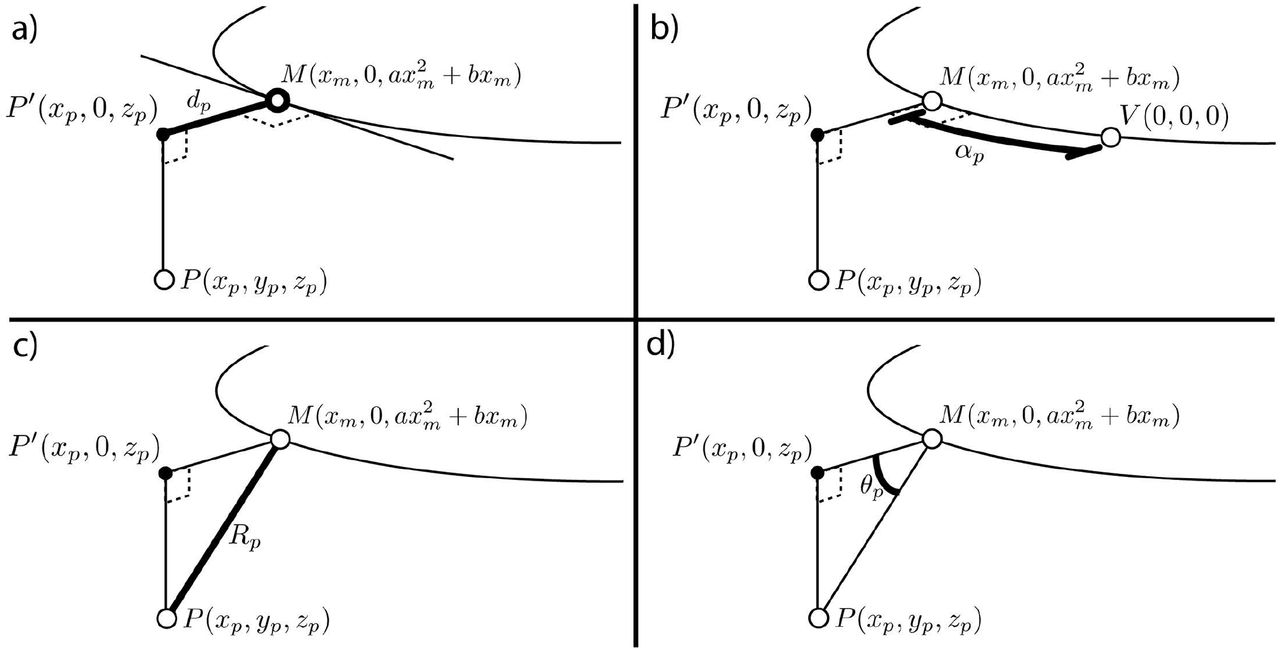
Given a data point P(xp, yp, zp) and a model of the commissure  , we calculate a cylindrical coordinate system that defines the position of P relative to M. a) First, we must identify the xm value which defines the point M(xm) that is closest to P. Since M lies in the X′Z′ plane where all y = 0, we can consider P as it lies in the X′Z′-plane, P′(xp, 0, zp). The distance between M and P′ (dp) is calculated by finding the Euclidean distance between the two points. We then use an optimization function to find the value of xm that minimizes dp. b) Given M(xm) that minimizes dp, the arclength distance between M and V(0,0,0) at the midline (αp) is found by calculating the integral of M between M(xm) and V. c) Given M(xm) that minimizes dp, the Euclidean distance (Rp) between M and P can be calculated in 3 dimensions. d) Finally, given dp and Rp, the angle of P(θp) can be calculated according to trigonometric rules.
In order to identify the value of xm, an optimization function from SciPy was used to minimize dp as a function of xm [33]. In other words, given a point P(x, y, z), find a value xm such that the distance between the projection of P to the X′Z′-plane and the point M(xm, 0, z(xm)) is minimized. αp was defined by calculating the distance along the model between M and the vertex V(0,0,0),
 (Fig 21 B). θp was calculated as follows:
 (Fig 21 D). Finally, R was calculated as the Euclidean distance between P and M in 3D space,
 (Fig 21 C). The probability density functions of each dimension in the cylindrical coordinate system (α,θ,R) were estimated using a kernel density estimate (KDE) [33]. A Gaussian kernel was used with the bandwidth selected according to Scott’s Rule [34].
After transforming the data to cylindrical coordinates, the dataset is saved to a PSI file according to PSI Format 1.0. Each point is assigned an ID number and the following values are saved: x, y, z, α, R, θ. The Cartesian coordinates correspond to the position of the data following sample alignment.
Landmark calculation
In order to perform statistical comparisons between samples, we reduced the sample data to a set of representative landmark points. The POC was divided into eight wedges around θ, each spanning 45º, and into nα slices along α. For each sample the number of points in each wedge was calculated and the 50th percentile (median) of the R values of the data determined. In order to identify landmarks that exhibited statistically significant differences in median radius across wild type and yot samples, a two-sided t-test was performed on each landmark bin. We are testing the null hypothesis that the distributions of median radius values are the same in wild type and mutant samples. Given that 88 landmarks are being tested, but variability and independent development exist between different landmarks, multiple testing solutions were needed to control the false positive rate. This was achieved by setting the minimum p-value to p¡.01, and counting as significant only bins with 2 adjacent significantly different bins.
Distribution and accessibility
The code base of ΔSCOPE is available online as a Python package hosted on the https://pypi.org/project/deltascope/ Python Package Index. The raw code repository is available on https://github.com/msschwartz21/deltascope Github, which records changes to the code and logs issues encountered by users of the code. In order to facilitate ease-of-use, extensive documentation of ΔSCOPE and its associated workflows is available on https://deltascope.readthedocs.io/en/latest/ Read the Docs.
Supporting information
S1 File. An archived copy of the ΔSCOPE code repository. The most up-to-date version of the code is available on https://github.com/msschwartz21/deltascopeGithub or for installation via https://pypi.org/project/deltascope/Python Package Index.
S2 File. A pdf copy of documentation that accompanies the ΔSCOPE code repository. Also available on https://deltascope.readthedocs.io/en/latest/ Read the Docs.
S1 Data. Data associated with the developmental timecourse analysis of the glial bridge and post-optic commissure. https://doi.org/10.35482/bld.003.2019
S2 Data. Data associated with the analysis of the role of S1a. https://doi.org/10.35482/bld.002.2019
Acknowledgments
We would like to thank the generous contributions of Melissa Hardy and the late Chi-Bin Chien to this research in their development and donation of the heatshock (hsp70) responsive slit1a tghsp70:slit1a:mcherry and tghsp70:mcherry lines. We would like to Nadia PenkoffLiedbeck, Cassie Kemmler, and Jin-Sook Park for their substantial contributions to data collection and project assistance. We would also like to thank Margaret Perry, Audrey Bertin, Kalynn Kosyka, Crystal Zang, Emma Ning for their assistance reviewing the code base and providing technical assistance weeding out errors. This work would not have been possible with out the generous contributions of time and effort by the Smith College Center for Microscopy and its director, Judith Wopereis, and the Smith Animal Care facility. We would also like to thank our funding sources at the NIH (HD060023) and NSF (IOS-1656310), as well as graduate student funding from the University of Massachusetts Amherst IDGP. We are very thankful for all of the technical support provided by Alicia Famiglietti and all constructive discourse by the entire Barresi lab throughout this work.
Footnotes
References


