

Abstract
How are actions linked with subsequent outcomes to guide choices? The nucleus accumbens (NAc), which is implicated in this process, receives glutamatergic inputs from the prelimbic cortex (PL) and midline regions of the thalamus (mTH). However, little is known about what is represented in PL or mTH neurons that project to NAc (PL-NAc and mTH-NAc). By comparing these inputs during a reinforcement learning task in mice, we discovered that i) PL-NAc preferentially represents actions and choices, ii) mTH-NAc preferentially represents cues, iii) choice-selective activity in PL-NAc is organized in sequences that persist beyond the outcome. Through computational modeling, we demonstrate that these sequences can support the neural implementation of temporal difference learning, a powerful algorithm to connect actions and outcomes across time. Finally, we test and confirm predictions of our circuit model by direct manipulation of PL-NAc neurons. Thus, we integrate experiment and modeling to suggest a neural solution for credit assignment.
Introduction
Multiple lines of experimental evidence indicate that the NAc (part of the ventral striatum) is critical to reward-based learning and decision making (Cox and Witten, 2019; Di Ciano et al., 2001; Parkinson et al., 1999; Roitman et al., 2005; Setlow et al., 2003; Stuber et al., 2011). The NAc is a site of convergence of glutamatergic inputs from a variety of regions, including the prefrontal cortex and the midline thalamus, along with dense dopaminergic inputs arising from the midbrain (Do-Monte et al., 2017; Hunnicutt et al., 2016; Otis et al., 2017; Poulin et al., 2018; Reed et al., 2018; Zhu et al., 2016).
An important mechanism underlying reward-based learning and decision making is thought to be dopamine-dependent synaptic plasticity of glutamatergic inputs to the NAc that are co-active with a reward prediction error (RPE) in dopamine neurons (Fisher et al., 2017; Gerfen and Surmeier, 2011; Reynolds and Wickens, 2002; Russo et al., 2010). Such strengthening of glutamatergic inputs is thought to be central to learning, allowing actions that are followed by reward to be more likely to be repeated in the future (Britt et al., 2012; MacAskill et al., 2014; Steinberg et al., 2013; Tsai et al., 2009; Witten et al., 2011).
A central question in reinforcement learning is how actions and outcomes become associated with each other, even when they are separated in time (Asaad et al., 2017; Gersch et al., 2014; Sutton, 1988; Wörgötter and Porr, 2005). A possible mechanism that could contribute to solving this problem of temporal credit assignment in the brain is that neural activity in the glutamatergic inputs to the NAc provide a neural memory trace of previous actions. This could allow action representations from glutamatergic inputs and outcome information from dopaminergic inputs to overlap in time.
Whether glutamatergic inputs to the NAc indeed represent memories of previous actions is unclear. More broadly, what information is carried by glutamatergic inputs to the NAc during reinforcement learning, and whether different inputs provide overlapping or distinct streams of information, has not been examined systematically. To date, there have been relatively few recordings of cellular resolution activity of glutamatergic inputs to the NAc during reinforcement learning, nor comparison of multiple inputs within the same task, nor examination of the timescale with which information is represented within and across trials. Furthermore, if glutamatergic inputs do indeed provide memories of previous actions, construction of a neurally plausible instantiation of an algorithm for credit assignment based on the measured signals remains to be demonstrated (for review of biological instantiation of reinforcement learning algorithms, see (Joel et al., 2002)).
To address these gaps, we combined a retrograde viral targeting strategy with cellular resolution imaging during a reinforcement learning task to examine and compare activity in major cortical and thalamic input to the NAc core: the input from prelimbic cortex (part of mPFC, “PL-NAc”) and that from the midline thalamus (“mTH-NAc”). We found that PL-NAc neurons preferentially encode actions and choices relative to mTH-NAc neurons, with choice-selective activity that persists until the start of the subsequent trial. The long timescale through which prior actions are encoded in cortical inputs to the NAc provides the information to bridge actions, outcomes, and subsequent choices. In addition, we demonstrated with computational modeling that these choice-selective sequences can contribute to a concrete neural instantiation of temporal difference (TD) learning, a powerful reinforcement learning algorithm that allows appropriate learning of the association of actions and outcomes separated in time. Finally, we test and confirm a prediction of our model through direct optogenetic manipulation of PL-NAc neurons. Thus, by recording and manipulating glutamatergic inputs to the NAc and integrating these data with computational modeling, we provide a specific proposal for how TD learning could be implemented by neural circuitry.
Results
Cellular resolution imaging of glutamatergic inputs to the NAc during a probabilistic reversal learning task
Mice performed a probabilistic reversal learning task while inputs from thalamus or cortex were imaged (Figure 1a). A trial was initiated when the mouse entered a central nose poke, which prompted the presentation of a lever on either side. Each lever had either a high (70%) or low (10%) reward probability, with the identity of the high and low probability levers reversing in an unsignaled manner after a variable number of trials (see Methods for block transition probabilities). After a variable delay (0-1s), either a sound (CS+) was presented at the same time as a reward was delivered to a central reward port, or another sound (CS–) was presented that signaled the absence of reward.

(a) Schematic of probabilistic reversal learning task. Animals began a trial by entering a central nose poke (nose poke’) which resulted in the presentation of two levers (‘levers out’). A lever press resulted in either a rewarded (CS+, reward consumption) or unrewarded (CS–) outcome, with the probability of a given outcome dependent on whether the trial was in a right or left high probability block. A high probability press (i.e. a left press in a left block, or a right press in a right block) led to reward on 70% of trials, while a low probability press led to reward on 10%. (b) Example behavior of a mouse performing 100 trials during a single recording session. The choice of the animal (black dots) follows the identity of the higher probability lever as it alternates between a left and right block (horizontal grey bars). (c) Left, Probability of the animals choosing either the left or right lever 10 trials before and after a switch from a left to right high probability block. Right, same as left except choice probabilities following a right to left high probability block (d). Animals had a significantly higher stay probability following a rewarded versus unrewarded trial (*** p=5×10⁻⁹, two-tailed t-test, n=16 mice) (e) Coefficients from a logistic regression that uses choice and outcome from the previous five trials to predict choice on each trial. The regression used two sets of predictors: (i) ‘Rewarded trials’ (green) which identify a previous trial as a rewarded right press (+1), rewarded left press (−1) or unrewarded press (0) and (ii) ‘Unrewarded trials’ (red), which identify a previous trial as an unrewarded right press (+1), unrewarded left press (−1) or rewarded trial (0). Positive regression coefficients correspond to a greater likelihood of the animal making a lever press with the same choice identity as that of the previous trial. c,d,e, error bars are s.e.m. across animals (n=16) (f) Left, surgical schematic for PL-NAc (top) and mTH-NAc (bottom) recordings showing the injection site and optical lens implant with miniature head-mounted microscope attached. Right, Coronal section from a PL-NAc (top) and mTH-NAc (bottom) animal showing GCaMP6f expression in each respective recording site. Inset: confocal image showing GCaMP6f expression in individual neurons. (g) Left, example field of view from a recording in PL-NAc (top, blue) and mTH-NAc (bottom, orange) with five representative regions of interest (ROIs). Right, normalized GCaMP6f traces from the five ROIs on the left. For visualization purposes, each trace was normalized by the peak fluorescence across the hour long session.
As expected, mice reversed the lever they were more likely to press following block transitions (Figure 1b,c). Similarly, mice were significantly more likely to return to a previously chosen lever (i.e. stay) following rewarded, as opposed to unrewarded, trials (Figure 1d; p<0.0001: paired, two-tailed t-test across mice, n=16 mice), meaning that, as expected, mice were using previous choices and outcomes to guide behavior. A logistic regression to predict choice based on previous choices and outcomes indicated that mice relied on ~3 previous trials to guide their choices (Figure 1e; see Methods for model details).
To image activity of glutamatergic input neurons to the NAc during this behavior, we injected a retroAAV or CAV2 virus expressing Cre-recombinase in the NAc as well as an AAV2/5 expressing Cre-dependent GCaMP6f in either the PL or mTH (Figure 1f). A GRIN lens was implanted above either the PL or mTH (see Supplementary Figure 1 for implant locations), and a head-mounted miniature microscope was used to image activity in these populations during behavior (Figure 1f, n=278 neurons in PL-NAc from n=7 mice, n=256 neurons in mTH-NAc from n=9 mice). An example field of view from a single recording session is shown for both PL-NAc neurons as well as mTH-NAc neurons (Figure 1g). Behavior between mice in the PL-NAc versus mTH-NAc cohorts was similar (Supplementary Figure 2).

(a) Schematic of coronal sections along the anterior/posterior axis (A/P, numbers relative to bregma) with recording locations of 7 PL-NAc animals. Red lines indicate bottom of lens implant. (b) Same as a except location of 9 mTH-NAc recordings.

(a) Top, regression coefficients from logistic regression model (see Figure 1) from PL-NAc cohort (n=7 mice). Bottom, same except coefficients from mTH-NAc cohort (n=9 mice). Both cohorts use choice and outcome information from the previous two trials to predict the current choice. Regression coefficients between the two cohorts are not significantly different for any trials back for either rewarded or unrewarded trials (P>0.01, unpaired, two-tailed t-test of regression coefficients across animals at each trial back, n=7 and 9 mice for PL-NAc and mTH-NAc, respectively). (b) Stay probability following rewarded (blue or orange) and unrewarded (grey) trials for PL-NAc (top) and mTH-NAc (bottom) cohorts. Both cohorts have a significantly higher stay probability following a rewarded trial (PL-NAc: P=0.00008; mTH-NAc: P=0.00003, paired, two-tailed t-test comparing stay probability on rewarded and unrewarded trials across mice, n=7 and 9 mice for PL-NAc and mTH-NAc, respectively). (c) Probability of a left or right lever press following a transition from a left-preferring to right-preferring block of mice from the PL-NAc (top, n=7 mice) and mTH-NAc (bottom, n=9 mice) cohorts. Both cohorts display similar change in choice behavior following a block transition. Error bars indicate s.e.m. across animals in all panels.
Actions are preferentially represented by PL-NAc neurons, while reward-predicting stimuli are preferentially represented by mTH-NAc neurons
Individual PL-NAc and mTH-NAc neurons displayed elevated activity when time-locked to specific events in the task (Figure 2a). To precisely relate neural activity to each event, we built an encoding model. Briefly, time-lagged versions of each behavioral event (nosepoke, lever press, etc) were used to predict the GCaMP6f signal in each neuron using a linear regression. This allowed us to obtain “temporal kernels”, which related each event to the GCaMP6f signal in each neuron, while reducing the contribution of the other events (Figure 2b; see Methods for model details).
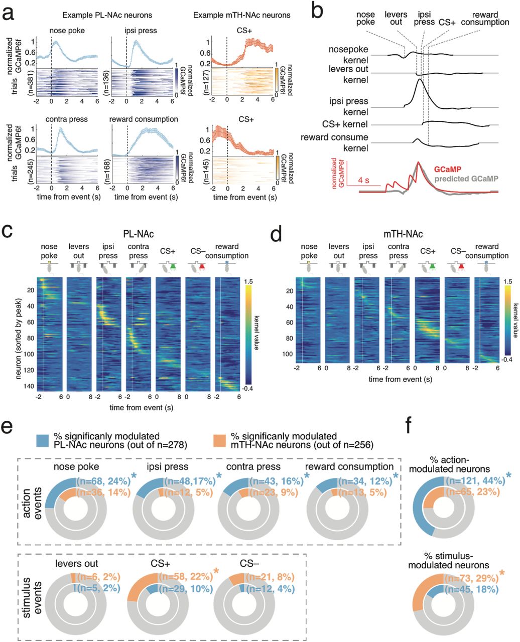
(a) Time-locked responses of individual PL-NAc (blue) and mTH-NAc (orange) neurons to task events. (b) Kernels representing the response to each of the task events for an example neuron, generated from the encoding model. The predicted GCaMP trace in the model is the sum of the individual kernels, aligned to the behavioral event times (see Methods). (c) All PL-NAc neurons with significant modulation to at least one event (n=143/278 neurons from 7 mice). Each row is a neuron and columns are the event kernels from the encoding model. The heatmap is ordered by the time of peak kernel response across all behavioral events. (d) Same as c, for mTH-NAc neurons that were significantly modulated by at least one event (n=109/256 neurons from 9 mice). (e) Proportion of neurons significantly modulated by each task event. PL-NAc population had a significantly larger fraction of neurons modulated by action events (‘nose poke’, ‘ipsilateral lever press’, ‘contralateral lever press’, ‘reward’) compared with mTH-NA. In contrast, mTH-NAc had a significantly larger fraction of CS+ modulated neurons compared with PL-NAc. Significance was determined using the linear model used to generate kernels in b, see Methods for additional model details. (f) Top, a greater proportion of PL-NAc neurons encode at least one action event (P=0.0002: two-proportion Z-test comparing proportion of action-modulatedP L-NAc and mTH-NAc neurons). Bottom, same as top except a larger proportion of mTH-NAc neurons encode a stimulus event compared with PL-NAc (P=0.0006: two-proportion Z-test comparing proportions of stimulus-modulated neurons between PL-NAc and mTH-NAc). e,f Asterisk indicates P<0.05, two-proportion Z-test comparing proportion of significantly modulated PL-NAc and mTH-NAc neurons.
This encoding model was used to identify neurons in the PL-NAc and mTH-NAc populations that were significantly modulated by each event in our task (significance was assessed by comparing the encoding model with and without each task event, see Methods). We found a slightly (but significantly) larger proportion of PL-NAc neurons were modulated by at least one task event relative to mTH-NAc (PL-NAc: n=143/278 neurons from 7 mice; mTH-NAc: n=109/256 neurons from 9 mice; P=0.041: two-proportion Z-test comparing proportions of significantly event-modulated neurons).
Interestingly, the selectivity for actions versus sensory stimuli clearly differed between the two populations (Figure 2c-f). In particular, more PL-NAc neurons were modulated by action events (nose poke: P=0.002, ipsi lever press: P=0.0002, contra lever press: P=0.02, reward consumption: P= 0.004, two-proportion Z-tests comparing proportion of action-modulated neurons in PL-NAc and mTH-Nac), while more mTH-NAc neurons were modulated by the reward-predictive cues (CS+: P= 0.0002, CS-: P=0.062, two-proportion Z-test comparing proportion of stimulus-modulated neurons in PL-NAc and mTH-NAc). Examination of the time-locked GCaMP6f fluorescence (rather than the encoding model) led to similar conclusions of preferential action representations in PL-NAc (Supplementary Figure 3).

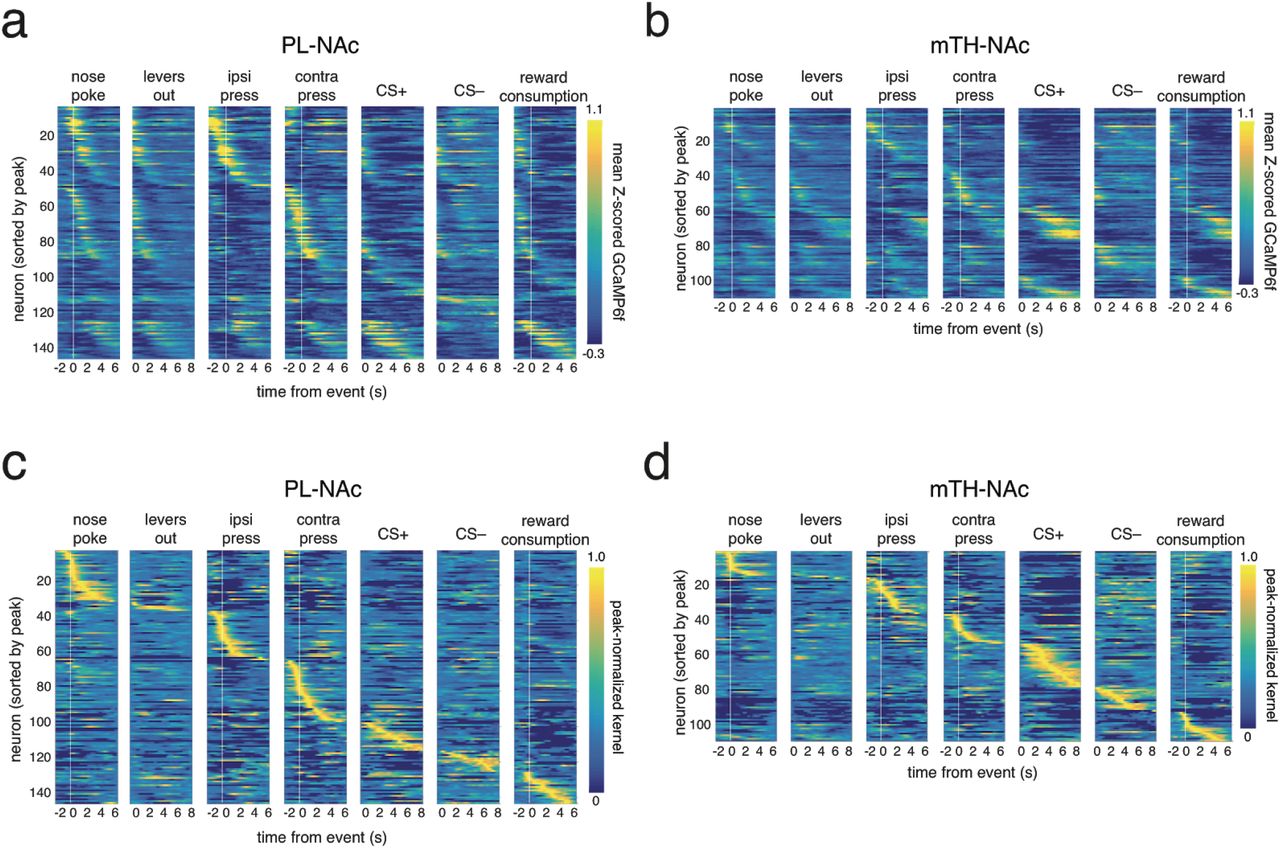
(a) Heatmap of event-modulated PL-NAc neurons’ mean Z-scored GCaMP6f response to each of the task events (n=143 neurons from 7 mice). (b) Same as a except response of event-modulated mTH-NAc neurons (n=109 neurons from 9 mice). The pattern of activation is qualitatively similar to that found using the regression model from Figure 2c,d. (c) Same as Figure 2c except each PL-NAc neuron’s kernels are normalized by the peak kernel value across all events. (d) Same as c except mTH-NAc.
PL-NAc neurons preferentially encode choice relative to mTH-NAc neurons
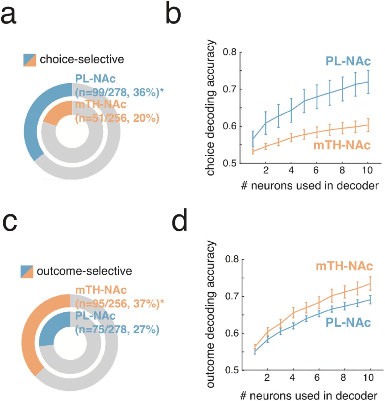
This preferential representation of actions in PL-NAc relative to mTH-NAc suggests that lever choice (contralateral versus ipsilateral to the recording site) could also be preferentially encoded in PL-NAc. Indeed, a significantly larger fraction of neurons were choice-selective in PL-NAc compared with mTH-NAc (Figure 3a; PL-NAc: 99/278 (36%); mTH-NAc: 51/256 (20%); P=0.00006: two proportion Z-test; significant choice-selectivity was determined with a nested comparison of the encoding model with and without choice information, see Methods). A population decoder supported this observation of preferential choice-selectivity in PL-NAc relative to mTH-NAc (Figure 3b; PL-NAc: 72±3%, mTH-NAc: 60±2%, choice decoding accuracy from a logistic regression with activity from multiple, random selections of 10 simultaneously imaged neurons, mean±s.e.m. across mice).

(a) Proportion of choice-selective neurons in PL-NAc (n=99 out of 278 neurons from 7 mice) and mTH-NAc (n=51 out of 256 neurons from 9 mice) (b) Choice decoding accuracy using neural activity from one to ten randomly-selected, simultaneously imaged neurons around the time of the lever press. The PL-NAc population (n=6 animals) more accurately decodes the choice of the trial compared with mTH-NAc (n=9 animals; peak decoding accuracy of 72+/-3% for PL-NAc and 60+/-2% for mTH-NAc). Error bars indicate s.e.m. across animals. (c) Proportion of outcome-selective neurons in PL-NAc (n=75 out of 278 neurons, n=7 mice) and mTH-NAc (n=95 out of 256 neurons, n=9 mice). (d) Outcome decoding accuracy using neural activity from one to ten randomly-selected, simultaneously imaged neurons after the time of the CS. The mTH-NAc population (n=9 animals) more accurately decodes the outcome of the trial compared with PL-NAc (n=6 mice; peak decoding accuracy of 74+/-2% for mTH-NAc and 69+/-1% for PL-NAc). Error bars indicate s.e.m. across animals.
In contrast to the preferential representation of choice in PL-NAc compared to mTH-NAc, a significantly larger fraction of neurons in mTH-NAc were outcome-selective compared with PL-NAc (Figure 3c; mTH-NAc: 95/256 (37%), PL-NAc: 76/278 (27%); P=0.01: two-proportion Z-test; significant outcome-selectivity was determined with a nested comparison of the encoding model with and without outcome information, see Methods). Similarly, outcome decoding in mTH-NAc was slightly better relative to PL-NAc (Figure 3d; mTH-NAc: 73±2%, PL-NAc: 69±1%: logistic regression to decode outcome with repeated random selections of 10 simultaneously imaged neurons, mean±s.e.m. across mice).
PL-NAc neurons display choice-selective sequences that persist into the next trial
We next examined the temporal organization of choice-selective activity in PL-NAc neurons. Across the population, choice-selective PL-NAc neurons displayed sequential activity with respect to the lever press that persisted for >4s after the press (Figure 4a,b). The robustness of these sequences was confirmed using a cross-validation procedure, in which the order of peak activity across the PL-NAc choice-selective population was first established using half the trials (‘training’), and then the population heatmap was plotted using the same established ordering and activity from the other half of trials (‘test’) (Figure 4b). To quantify the consistency of these sequences, we correlated the neurons’ time of peak activity in the ‘training’ and ‘test’ data, and observed a strong correlation (Figure 4c; R2=0.829, P=3×10⁻²⁶, n = 99 neurons from 7 mice) indicating that the temporal properties of choice-selective PL-NAc neurons were consistent across trials. In contrast, choice-selective sequential activity in the mTH-NAc population was significantly less consistent than PL-NAc (Supplementary Figure 4; P=0.007, Z=2.7: Fisher’s Z, comparison of correlation coefficients derived from comparing peak activity between ‘test’ and ‘training’ data from PL-NAc versus mTH-NAc).

(a) Left, heatmap of choice-selective mTH-NAc neurons’ peak-normalized GCaMP6f response to the ipsilateral (left column) and contralateral (right column) lever press using ‘train data’ from half of trials and sorted by the time of peak activity (n=51 neurons from 9 mice). Right, same as left only heatmap is made using ‘test data’ taken from other half of trials while maintaining the order from the ‘train data’. Compare to PL-NAc data in Figure 4b. (b) Correlation between the time of peak activity using the ‘train’ (horizontal axis) and ‘test’ (vertical axis) trials for choice-selective mTH-NAc neurons. While mTH-NAc choice-selective neurons also show significant correlation between ‘train’ and ‘test’ trials (R2 = 0.61, P = 0.000002, n=51 neurons from 9 mice), this correlation is lower than that of PL-NAc (comparison with data in Figure 4c;). (c) Top; average GCaMP6f activity of three simultaneously imaged mTH-NAc choice-selective neurons with different response times relative to the lever press. Error bars are s.e.m across trials. Bottom, heatmaps of response across trials to ipsilateral (orange) and contralateral press (grey) (d) Average decoding accuracy of the current (orange), previous (grey) and future trial (black) using activity from 10 simultaneously imaged mTH-NAc neurons as a function of time throughout the trial. Error bars are s.e.m. across 9 animals. Dashed black lines indicate time of events used to time-stretch neural activity (see methods for details). Red dashed line indicates median time of reward consumption.

(a) Top; average GCaMP6f activity of three simultaneously imaged PL-NAc choice-selective neurons with different response times relative to the lever press. Error bars are s.e.m across trials. Bottom, heatmaps of GCaMP6f fluorescence across trials to ipsilateral (blue) and contralateral press (grey) (b) Heatmaps demonstrating sequential activation of choice-selective PL-NAc neurons (n=99/278 neurons). Each row is the average GCaMP6f activity time-locked to the ipsilateral (left column) and contralateral (right column) lever press for a neuron, normalized by the neuron’s peak average fluorescence. Left, heatmap was first ordered using ‘training data’ from half of trials and sorted by the time of peak activity. Right, same as left only heatmap is made using ‘test data’ taken from other half of trials while maintaining the order from the ‘train data’. (c) High degree of correlation between the time of peak activity using the ‘train’ (horizontal axis) and ‘test’ (vertical axis) trials for choice-selective PL-NAc neurons (R2 = 0.83, P = 3×10⁻²⁶, n = 99 neurons). (d) Average choice decoding accuracy as a function of GCaMP6f activity throughout the trial, from 100 random selections per mouse of 10 simultaneously imaged PL-NAc neurons (each trial’s activity is aligned relative to the events demarcated with the vertical dashed black lines, see Methods). Error bars are s.e.m. across mice (n=6). Red dashed line indicates median onset of reward consumption.
A striking feature of the choice-selective sequences in PL-NAc was that they persisted for seconds after the choice, potentially providing a neural ‘bridge’ between action and outcome. To further quantify the timescale of choice encoding, both within and across trials, we used activity from simultaneously imaged neurons at each timepoint in the trial to predict the animal’s choice (with a decoder based on a logistic regression using random combinations of 10 simultaneously imaged neurons to predict choice). Choice on the current trial could be decoded above chance for ~9s after the lever press, spanning the entire trial (including the time of reward delivery and consumption), as well as the beginning of the next trial (Figure 4d). Choice on the previous or subsequent trial was not represented as strongly as current trial choice (Figure 4d; in all cases we corrected for cross-trial choice correlations with a weighted decoder, see Methods). We also examined the temporal extent of choice encoding in the mTH-NAc population (Supplementary Figure 4c,d). Similar to PL-NAc, we observed that decoding of the animals’ choice persisted up to the start of the next trial. However, the peak decoding accuracy across all time points in the trial was lower in mTH-NAc (59%±0.2%) compared with PL-NAc (73±0.2%).
Choice-selective sequences in PL-NAc neurons, in combination with known anatomy, can provide a substrate for temporal difference (TD) learning
Thus far, we observed that choice-selective sequences in PL-NAc neurons encoded the identity of the chosen lever for multiple seconds after the lever press. This sequential activity bridged the gap in time between an animal’s action and reward feedback, and therefore contained information that could be used to solve the task (Figure 4b,d). But how could a biologically realistic network use sequences to implement this task? In particular, how could PL-NAc neurons (and their synapses) that were active at the beginning of the choice-selective sequence - and were presumably important to initiating the sequence - be strengthened by an outcome that occurred toward the end of the sequence?
To address this question, we developed a biologically realistic computational model that could perform this task based on the observed choice-selective sequences in PL-NAc neurons. This was achieved using a model that implemented a temporal difference (TD) reinforcement learning algorithm by combining the recorded choice-selective sequential activity of PL-NAc neurons with the known connectivity of downstream structures (Figure 5a-c). The goal of TD learning is for weights to be adjusted in order to predict the sum of future rewards, or “value”, as well as possible (Dayan and Niv, 2008; O’Doherty et al., 2003; Sutton et al., 1998; Tsitsiklis and Van Roy, 1997). The error signal in this algorithm, which adjusts weights at each time step, is the difference between experienced and expected reward. In this algorithm, the expected reward is estimated as the difference in value at neighboring time points, and is the source of the term “temporal difference”. (This difference in value at neighboring time points estimates expected reward because value is the sum of all future rewards.) The error signal in this algorithm closely resembles the RPE signal observed in ventral tegmental area (VTA) dopamine neurons(Bayer and Glimcher, 2005; Schultz, 1998; Schultz et al., 1997), but how this signal is computed remains an open question.

(a) Schematic of circuit architecture used in the model. Choice-selective PL neurons, each with a sequential temporal activity pattern defined as  for right-preferring neurons and
  for left-preferring neurons, form synapses with GABAergic NAc projection neurons with weights
  and
and  . Assuming that dopamine neuron provide an RPE signal δ(t), the strength of PL-NAc synapses would be modified to reflect value at the time point that the corresponding PL-NAc neuron is active. This results in temporally-restricted value signals in NAc neurons, which after undergoing a sign inversion in the ventral pallidum (VP), projects to both a GABA interneuron as well as a dopamine neuron in the VTA. The activity within the GABA VTA interneuron thus represents the sum of activity across all NAc neurons at a given time point, t, which is representative of the total value function at that time. Therefore, the dopamine neuron computes a TD error, δ(t), based on the direct input from the VP neurons, which signals value, along with the temporally delayed value signal arising from the synapse from the GABA interneurons, and a reward input r(t). (b) Equations for the model as instantiated by the circuit schematic in a. Here α defines the learning rate, τ(c) defines the decay time constant for the PL-NAc synaptic eligibility trace E(t), Δ is the delay generated by the VTA GABA interneuron, is the discount in value associated with a time step Δ, nL,r is the total number of left and right-preferring neurons respectively. The individual sums of left and right-preferring NAc neuron activity is given by QL and QR, respectively, and the sum of the left and right value is Q. (c) Heatmap of PL-NAc firing rates used as input to the model. Firing rates estimated from GCaMP6f activity in Figure 4b. (d) Behavior of the TD model for a series of high probability block reversals. The decision variable (red trace) along with the predicted choice of the model (black dots) follows the identity of the higher probability lever as it alternates between a left and right block (horizontal grey bars) (e) Predicted stay probability of the TD model following rewarded and unrewarded trials. Similar to the behavior of mice in Figure 1d, the model predicts a higher stay probability following a rewarded trial compared with an unrewarded trial. (f) Simulated VTA dopamine neuron activity, generated by averaging across rewarded trials, top, and unrewarded trials, bottom. (g) Top, coefficients from a linear regression that uses outcome of the current and previous six trials to predict δ(t) during reward feedback. Bottom, same as top, except outcome history predicts δ(t) in the time prior to reward feedback. Both set of coefficients follow pattern predicted by the encoding of an RPE as observed in recorded dopamine activity (see Supplementary Figure 5 for experimental recordings). (h) Control model was designed such that the PL-NAc neurons fire synchronously at the onset of the sequence (2.5s before the lever press), rather than sequentially. (i-l) same as d-g, except results from using the control model with synchronous PL-NAc activity. Unlike the sequential model, synchronous PL-NAc activity is not able to generate appropriate behavior (i-j) nor is it able to produce an RPE signal (k-l).

(a) Coefficients from a linear regression similar to that in Figure 5g,l, except outcome history predicts recorded GCaMP6f in VTA-NAc dopaminergic terminals to CS presentation, data from Parker et al. (2016). The positive coefficient for the current trial and negative coefficients for previous trials indicate the encoding of an RPE reward prediction error. Error bars represent s.e.m across 11 recording sites. (b) Same as a except linear model predicts average VTA-NAc dopamine activity before the CS presentation. The positive coefficients corresponding to outcome on previous trials indicates an increase in dopamine activity following reward, consistent with the encoding of an RPE reward prediction error signal.
In our model, the PL-NAc sequences enabled the calculation of the TD error in dopamine neurons. Over the course of a series of trials, this error allowed a reward that occurred at the end of the PL-NAc sequence to adjust synaptic weights at the beginning of the sequence (Figure 5a-c). Our model generated a TD error in dopamine neurons based on minimal assumptions: i) the choice-selective sequences in PL-NAc neurons that we report here, ii) established (but simplified) anatomical connections between PL, NAc, and VTA neurons (see circuit diagram in Figure 5a), and iii) dopamine- and activity-dependent modification of the synapses connecting PL and NAc neurons (with a synaptic eligibility decay time constant of 0.5s, consistent with (Gerstner et al., 2018) and (Yagishita et al., 2014)).
In more detail, our model consisted of choice-selective and sequentially active PL neurons that formed synapses with NAc neurons, with the strength of each synapse modified in an activity-dependent manner by dopamine inputs from the VTA (Figure 5a). Assuming a TD error in the dopamine neurons, this would lead to neurons in NAc (and its synaptic target, the ventral pallidum, VP) acquiring activity that correlated with the value of either the left or right choice, with temporally restricted periods of activation determined by the timing of the sequential activation of the PL neuron that innervated them. The VP neurons sent convergent projections to the GABA interneuron and dopamine neurons in the VTA. These GABA interneurons therefore encoded value at every time point, as they received convergent input from neurons that encoded value transiently. In addition to the convergent VP inputs, the VTA dopamine neurons received a direct reward signal, as well as an input from the GABA interneurons of the VTA (which provided a synaptically delayed and inverted version of the VP signal - in other words, the GABA inputs performed the “temporal differencing” operation). Critically, these three inputs onto the dopamine neuron composed the three components of the TD error signal with the correct signs: reward, value, and an inverted and delayed value signal (Figure 5b). Thus, dopamine neurons carried a formal TD error, which enabled them to properly modify PL-NAc synapses at the beginning of the sequence. This synaptic modification enables the NAc neurons to encode value, providing a substrate for the selection of proper choice based on previous trial outcomes.
Thus, our model performed the task appropriately, both across blocks and on a trial-by-trial basis (Figure 5d,e comparison to Figure 1b,d; choice based upon a probabilistic readout of the difference between right and left values at the start of the sequence, see Methods). Appropriate task performance was achieved due to the calculation of a TD RPE signal in VTA dopamine neurons. The RPE signal was evident within a trial, based on the positive response to reward and negative response to unrewarded outcomes (Figure 5f). The RPE signal was also evident across trials, based on the negative modulation of the dopamine outcome signal by previous trial rewards, and by the positive modulation of the pre-outcome signal by previous trial rewards (Figure 5g, multiple linear regression similar to (Bayer and Glimcher, 2005; Parker et al., 2016), compare to recorded dopamine activity in NAc in Supplementary Figure 5).
The model also generated neural activity of the NAc/VP and GABA interneurons that was in agreement with previous reports (Cohen et al., 2012; Kim et al., 2009; Roesch et al., 2009; Tian et al., 2016). NAc neurons displayed transient and sequential value-related activity (Supplementary Figure 6a). The NAc/VP activity was transient and sequential because neurons were active primarily when the corresponding PL input neuron in the sequence was active, and activity correlated with value due to the PL-NAc weights being modified by the RPE signal in dopamine neurons (correlation with choice value was evident by the fact that activity depended on the identity of the high probability lever). The VTA GABA interneuron, instead, had a sustained value signal, due to the converging input of the transient, sequential value signals from NAc/VP (Supplementary Figure 6b). Note that a sustained value signal in VTA GABA interneurons and a transient value signal in the NAc/VP was reported in a recent study recording from monosynaptic inputs to the VTA dopamine neurons (Tian et al., 2016).

(a) Heatmaps of average activity relative to the time of the lever press of NAc projection neurons in the sequential TD model from Figure 5a across different trials within a block. Top row is the average activity across the first trials in a block (early trials), middle row from the fourth trials (middle trials) and bottom row from the last trials (late trials). Each column is average activity from trials from different block/ press combinations. For each subplot, the left-preferring neuron are ordered first, and the right preferring are ordered last. The activity of these left- and right-preferring NAc neurons increases throughout a block of their respective lever preference. In contrast, their activity decreases throughout a block opposite to their lever preference. (b) Average activity of our model’s VTA GABA interneuron (Figure 5a) relative to the time of the lever press across the same early, middle and late trials. Similar to a, throughout a left block (left column), the activity on left press trials increases from early to late trials while activity on right presses decreases. The opposite pattern is seen for left and right press trials throughout a right block (right column). (c) Same as a except NAc projection activity using synchronous PL-NAc activity. Unlike the sequential model, NAc projection activity on right and left trials is not modulated throughout a given block. (d) Same as b except VTA interneuron activity generated using synchronous model.
The choice-selective sequences in PL-NAc neurons were critical to model performance, as they allowed the backpropagation of the RPE signal across trials. This was verified by comparing the performance of the model using PL-NAc activity that was altered to be synchronously active at the sequence onset (Figure 5h). Unlike the sequential case, synchronous PL-NAc activity was unable to correctly modulate lever value following block transitions, and therefore did not lead to correct choices (Figure 5i,j). This was due to the fact that the synchronous model was unable to generate an RPE signal that was modulated properly within or across trials. Within a trial, negative outcomes did not result in the expected decrease in the dopamine signal (Figure 5k), while across trials, the influence of the previous trial’s reward on the dopamine signal was disrupted relative to both the sequential model and recorded dopamine activity (Figure 5l, compare to Figure 5g and recorded dopamine activity in NAc in Supplementary Figure 5).
Activation of PL-NAc neurons decreases the effect of previous trial outcomes on subsequent choice in both the model and the mice
We next sought to generate experimentally testable predictions from our model by examining the effect of disruption of these sequences on behavioral performance (Figure 6a,b). Towards this end, we replaced the PL-NAc sequential activity in the model with constant, population-wide and choice-independent activity on a subset of trials (10% of trials; Figure 6a). This generated a decrease in the probability of staying with the previously chosen lever following rewarded trials and an increase following unrewarded trials (Figure 6c). In other words, the effect of previous outcome on choice was reduced when PL-NAc activity was disrupted. In contrast, activation did not result in a difference in stay probability on the trial with activation, as choice was determined by spontaneous activity before the sequence initiates in PL-NAc neurons, combined with the synaptic weights between PL and NAc neurons (Figure 6d).
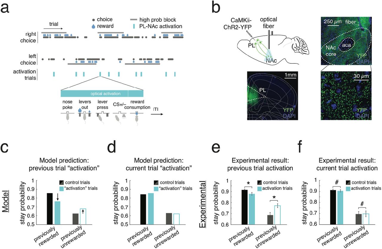
(a) In the model and in mice, PL-NAc neurons were activated synchronously and continuously on a randomly selected 10% of trials, disrupting the endogenous choice-selective sequential activity. For the model, activation began at the start of the sequence (2.5s before lever press) and lasted until the end of the trial (4s after lever press). For the experimental data, ChR2 activation (447 nm, 20 Hz stimulation, 5 ms pulse duration, 1-3 mW) began when the animal entered the central nose poke and continued until either 2s after the time of the CS or the end of reward consumption, depending on the outcome of the trial and the experimental cohort (see Methods and Supplementary Figure 7 for details). (b) Top, surgical schematic illustrating injection site of an AAV2/5 expressing ChR2-YFP in the PL (black needle) and optical fiber implant in the NAc core terminals. Bottom left, coronal section showing ChR2-YFP expression in PL. Bottom right, ChR2-YFP terminal expression in the NAc-core. (c) For the model, effect of previous trial activation on stay probability on the subsequent trial. Activation on a rewarded trial decreased stay probability on the subsequent trial, while activation on an unrewarded trial increased stay probability. (d) Same as c, except effect of activation on stay probability on the activated trial. For both rewarded and unrewarded trials, activation had no effect on stay probability on the stimulated trial. (e) Stay probability of mice following PL-NAc ChR2 activation. Activation on rewarded trials reduced stay probability on the subsequent trial (P = 0.002, paired, two-tailed t-test, n=14 mice). In contrast, activation on unrewarded trials caused animals to be more likely to stay with the previously chosen lever (P = 0.0005, paired, two-tailed t-test, n=14 mice). (f) Same as e, except effect of activation on stay probability on the activation trial. Activation caused no significant effect on stay probability following rewarded (P = 0.62, paired, two-tailed t-test, n=14 mice) or unrewarded trials (P = 0.91, paired, two-tailed t-test, n=14 mice). Error bars represent s.e.m. across animals.
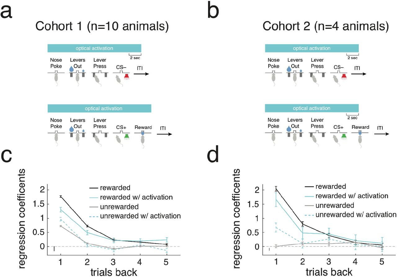
(a) Schematic of optical activation parameters for cohort 1. On 10% of unrewarded trials, optical activation began when the animal entered the central nosepoke and ended 2s after the end of the 500ms CS– tone. On 10% of rewarded trials, activation began with nose poke and ended after the animal left the reward port. (b) Schematic for cohort 2. Unlike cohort 1, optical activation ended on the same timescale on both rewarded and unrewarded trials – 2s after the end of CS presentation. (c) Logistic regression model similar to that in Figure 1e demonstrating effect of PL-NAc activation on lever choice cohort 1 animals (n=10 mice, see Methods for model details). Rewarded trials with activation one and two trials back decreased stay probability compared with rewarded trials without activation. Activation had an opposite effect on unrewarded trials, where there was an increase in stay probability following activation one trial back compared to trials without activation. (d) Same as c except data from cohort 2 (n=4 mice). Effect of optical activation of PL-NAc neurons was qualitatively similar across the two cohorts.
We tested these predictions experimentally by performing an analogous manipulation in mice, which involved activating PL-NAc axon terminals with ChR2 on 10% of trials. In close agreement with our model, mice had a significant decrease in stay probability following a rewarded trial that was paired with activation (Figure 6e; P=0.001: paired, two-tailed t-test, comparison between stay probability following rewarded trials with and without activation) and were more likely to stay following an unrewarded trial paired with activation (Figure 6e; P=0.0005: paired, two-tailed t-test, comparison between stay probability following unrewarded trials with and without activation). In contrast, activation on the current trial had no significant effect on stay behavior following either rewarded or unrewarded trials (Figure 6f; P>0.5: paired, two-tailed t-test, comparison between stay probability on trials with and without activation following both rewarded and unrewarded trials). We also observed an increase in the probability of the animals abandoning the trials with activation compared with those trials without, suggesting that this manipulation had some influence on the mouse’s motivation to perform the task (P=0.0006: paired, two-tailed t-test comparing percentage of abandoned trials on activated versus non-activated trials; 12.2+/-2.5% for activated trials, 0.9+/-0.2% for non-activated trials).
Discussion
This work provides both experimental and computational insights into how the NAc and associated regions could contribute to reinforcement learning. Experimentally, we found that mTH-NAc neurons are preferentially modulated by a reward-predictive cue, while PL-NAc neurons more strongly encoded actions (e.g. nose poke, lever press). In addition, PL-NAc neurons display choice-selective sequential activity which persists for several seconds after the lever press action, beyond the time the animals receive reward feedback. Computationally, we demonstrate that the sequential nature of PL-NAc activity can contribute critically to task performance, by implementing a biologically plausible version of TD learning (Sutton et al., 1998; Tesauro, 1992). Despite its simplicity, the model is able to i) perform the task, ii) replicate previous recordings in neurons across the circuit (i.e. VTA dopamine, VTA GABA, and NAc/VP neurons), and iii) make new predictions that we have experimentally tested on the effect of perturbing PL-NAc activity on trial-by-trial learning. Thus, this work suggests a computational role of choice-selective sequences, a form of neural dynamics whose ubiquity is being increasingly appreciated (Harvey et al., 2012; Long et al., 2010; Ölveczky et al., 2011; Pastalkova et al., 2008; Picardo et al., 2016; Sakata et al., 2008; Terada et al., 2017).
Relationship to previous neural recordings in the NAc and associated regions
To our knowledge, a direct comparison at cellular resolution of activity across multiple glutamatergic inputs to the NAc has not previously been conducted. This is a significant gap, given that these inputs are thought to contribute critically to reinforcement learning by providing the information to the NAc that dopaminergic inputs can reinforce (Centonze et al., 2001; Nestler, 2001; Nicola et al., 2000; Shen et al., 2008; Wilson, 2004; Xiong et al.). The differences in the representations in the two populations that we report were apparent due to the use of a behavioral task with both actions and sensory stimuli – in contrast to previous studies that employed Pavlovian tasks (Otis et al., 2017, 2019; Zhu et al., 2018).
The preferential representations of actions relative to sensory stimuli in PL-NAc is somewhat surprising, given that previous studies have focused on sensory representations in this projection (Otis et al., 2017), and also given that the NAc is heavily implicated in Pavlovian conditioning (Day and Carelli, 2007; Day et al., 2006; Di Ciano et al., 2001; Parkinson et al., 1999; Roitman et al., 2005; Wan and Peoples, 2006). On the other hand, there is extensive previous evidence of action correlates in PFC (Cameron et al., 2019; Genovesio et al., 2006; Luk and Wallis, 2013; Siniscalchi et al., 2019; Sul et al., 2010), and NAc is implicated in operant conditioning in addition to pavlovian conditioning (Atallah et al., 2007; Cardinal and Cheung, 2005; Collins et al., 2019; Hernandez et al., 2002; Kelley et al., 1997; Kim et al., 2009; Salamone et al., 1991).
The presence of choice-selective sequences in PL is reminiscent of previous reports in other behaviors in other regions of cortex, as well as in the hippocampus (Harvey et al., 2012; Pastalkova et al., 2008; Terada et al., 2017). In fact, given previous reports of choice-selective sequences in multiple brain regions and species (Long et al., 2010; Ölveczky et al., 2011; Picardo et al., 2016; Sakata et al., 2008), the relative absence of sequences in mTH-NAc neurons may be more surprising than the presence in PL-NAc. Interestingly, a study that recorded in another region of thalamus (Schmitt et al., 2017), as well as a study that recorded in dorsal striatum (Akhlaghpour et al., 2016), did not report sequential choice-selective activity (in the setting of other decision making tasks). Taken together, this may suggest that sequential choice-selective activity is less widespread in thalamus and striatum as in cortex and hippocampus.
The representation of the reward-predicting stimulus in mTH-NAc is in alignment with previous studies that have examined sensory representations in mTH structures (although, to our knowledge, the strength of action versus stimulus representations had not been directly examined). In particular, a previous study observed pronounced encoding of task-related stimuli in the centromedial thalamus of primates (Matsumoto et al., 2001). In this same study, encoding of these stimuli by striatal neurons was reduced following ablation of the thalamus. Together with our data, this suggests that the thalamus is contributing information about task-relevant stimuli to the striatum, which is likely critical for pavlovian conditioning (Campus et al., 2019; Do-Monte et al., 2017; Otis et al., 2019; Zhu et al., 2018).
Choice-selective sequences implement TD learning in a simple model that replicates and integrates numerous experimental findings
Given the widespread observation of choice-selective sequences across multiple behaviors and brain regions, including the PL-NAc neurons that we record from in this study, a fundamental question is what is the computational function of such sequences. Here, we suggest that these sequences may contribute to the neural implementation of TD learning, by providing a temporal basis set that bridges the gap in time between actions and outcomes.
A key idea of the model is that neurons active in a sequence that ultimately results in reward enable the backpropagation in time of the dopaminergic RPE signal, due to the fact that the earlier neurons in the sequence predict the activity of the later neurons in the sequence, which themselves overlap with reward. This causes synaptic weights onto NAc of these earlier neurons to be strengthened, which in turn biases the choice towards that represented by those neurons. Confirming the importance of the sequential nature of PL-NAc activity, when the model instead receives synchronous, rather than sequential PL-NAc activity, it fails to perform the task appropriately (Figure 5h-l).
Despite the fact that our model is constrained only by the PL-NAc activity we recorded and a simplified version of the downstream connectivity, it replicates numerous experimental findings. The most obvious is the calculation of an RPE signal in dopamine neurons (Bayer and Glimcher, 2005; Hart et al., 2014; Hollerman and Schultz, 1998; Schultz et al., 1997), which allows proper value estimation and, thus, task performance.
The key to the model producing an RPE signal in dopamine neurons is the GABA interneuron in the VTA, which generates the “temporal differencing” of the value inputs from VP, based on the sign inversion and temporal delay generated by the presence of a VTA GABA interneuron (Figure 5a). Although previous work had suggested other neural architectures for this temporal differencing operation (Hazy et al., 2010; Joel et al., 2002; Suri and Schultz, 1998, 1999), these models have not been revisited in light of recent cell-type and projection-specific recordings in the circuit. In fact, our architecture is motivated by new data. For example, electrical stimulation of VP generates both immediate inhibition of dopamine neurons, and delayed excitation, as required by our model (Chen et al., 2019). In addition, GABA interneurons encode value (Cohen et al., 2012; Tian et al., 2016), as predicted by our model, and their activation inhibits dopamine neurons, again consistent with our model (Eshel et al., 2015).
In addition, despite its simplicity, our model appears to explain some puzzling recent observations in the circuit: why do the NAc/VP neurons display temporally heterogeneous value representations, while the VTA dopamine and GABA interneurons have pure (and homogeneous) RPE and value signals, respectively (Adler et al., 2012; Cohen et al., 2012; Tian et al., 2016)? In fact, our model produces value signals in the NAc/VP that are transient and sequential due to the sequential nature of the PL input, whereas it produces a value signal in the GABA interneuron in the VTA that is sustained due to integrating inputs from the NAc/VP neurons. To our knowledge, this is the first model to predict heterogeneous value signal in the inputs to the VTA and the sustained value signal in the VTA GABA interneurons. However, our model does not completely predict the relative timing and sign of the value correlates in the NAc versus the VP (Tian et al., 2016), likely because of anatomical connections that we omitted from our circuit for simplicity (e.g.VP→ NAc, (Ottenheimer et al., 2018; Wei et al., 2016)).
Besides linking to recent data, another aspect that is attractive about our specific proposal for temporal differencing by the VTA GABA interneuron is that it could provide a generalizable mechanism for calculating RPE: it could extend to any input that projects both to the dopamine and GABA neurons in the VTA, and that also receives a dopaminergic input.
In addition to reproducing multiple previous experimental observations, our model also makes new and testable predictions, one of which we have tested in this paper. Specifically, in the model, overwriting the choice-selective sequential activity with continuous and synchronous activity in PL-NAc neurons disrupts the model’s ability to link choice and outcome on one trial to guide choice on the subsequent trial (Figure 6c). Optogenetic activation of PL-NAc activity adheres to this model prediction (Figure 6e). In contrast to the effect of stimulation on subsequent trial choice, stimulation causes no disruption of choice on the stimulated trial, in either the model or the experiment (Figure 6d,f). This is true in the model because choice is determined by the PL-NAc weights at the beginning of the trial, which are determined by previous trials’ choices and outcomes. Thus, the model provides a mechanistic explanation of a puzzling experimental finding: that optogenetic manipulation of PL-NAc neurons affects subsequent choices but not the choice on the stimulation trial itself.
Potential extensions of our model
TD learning based on a stimulus representation of sequentially active neurons has previously been proposed for learning a behavioral sequence (Fee and Goldberg, 2011; Jin et al., 2009), and for learning the timing of a CS-US relationship (Gershman et al., 2014). Here, we extend these ideas in the setting of a biologically constrained network model for driving appropriate choice behavior that depended on linking actions with subsequent outcomes.
For simplicity, we did not include mTH-NAc neurons in our model because the behavioral task involves learning which choice to make, and the mTH-NAc population had a relatively weak choice signal. The mTH-NAc inputs would instead be relevant had the goal of the task been to bridge a delay between a CS and a US (i.e. a pavlovian rather than an operant task), and including the thalamic input into this model is thus an obvious future extension.
Another element of the circuit that we did not include in this model is the indirect feedback loops from the basal ganglia back to mPFC. Inclusion of this feedback would produce representations of value and not just choice in mPFC, consistent with previous observations (Bari et al., 2019; Gläscher et al., 2009; Grabenhorst and Rolls, 2011; Kim et al., 2008). These value representations may bias choice via projections to the dorsal striatum (Bari et al., 2019). In addition, the indirect feedback from the NAc back to mPFC could also contributes to the formation of the PL sequences in the first place, with NAc activity at one time point helping to trigger cortical activity at the next time point. Further experiments and model extensions will be needed to explore these ideas.
Methods
Mice
30 male C57BL/6J mice aged 6-10 weeks from The Jackson Laboratory (strain 000664) were used for these experiments. Prior to surgery, mice were group housed with 3-5 mice/cage. To prevent mice from damaging the implant of cagemates, all animals used in imaging experiments were single housed post-surgery. All animals were kept on a 12-h on/ 12-h off light schedule. All experiments and surgeries were performed during the light off time. All experimental procedures and animal care was performed in accordance with the guidelines set forth by the National Institutes of Health and were approved by the Princeton University Institutional Animal Care and Use Committee.
Probabilistic reversal learning task
Beginning three days prior to the first day of training, mice were placed on water restriction and given per diem water to maintain >80% original body weight throughout training. Mice performed the task in a 21 x 18 cm operant behavior box (MED associates, ENV-307W). A shaping protocol of three stages was used to enable training and discourage a bias from forming to the right or left lever. In all stages of training, the start of a trial was indicated by illumination of a central nose poke port. After completing a nose poke, the animal was presented with both the right and left lever after a temporal delay drawn from a random distribution from 0 to 1s in 100 millisecond intervals. The probability of reward of these two levers varied based on the stage of training (see below for details). After the animal successfully pressed one of the two levers, both retracted and, after a temporal delay drawn from the same uniform distribution, the animals were presented with one of two auditory cues for 500ms indicating whether the animal was rewarded (CS+, 5 kHz pure tone) or not rewarded (CS–, white noise). Concurrent with the CS+ presentation, the animal was presented with 6μl of 10% sucrose reward in a dish located equidistantly between the two levers, just interior to the central nose poke. In all stages of training, a 2s intertrial interval which began either at the end of CS on unrewarded trials or at the end of reward consumption on rewarded trials. The end of reward consumption was defined as the animal being disengaged from the reward port for 100ms.
In the first stage of training (“100-100 debias”), during a two hour session, animals could make a central nose poke and be presented with both the right and left levers, each with a 100% probability of reward. However, to ensure that animals did not form a bias during this stage, after five successive presses of either lever the animal was required to press the opposite lever to receive a reward. In this case, a single successful switch to the opposite lever returned both levers to a rewarded state. Once an animal received >100 rewards in a single session they were moved to the second stage (“100-0”) where only one of the two levers would result in a reward. The identity of the rewarded lever switched after 10 rewarded trials plus a random number of trials drawn from a geometric distribution of p = 0.4 (mean 2.5). On average, there were 23.23 +/-7.93 trials per block and 9.67 +/-3.66 blocks per session. After 3 successive days of receiving >100 rewards, the mice were moved to the final stage of training (“70-10”), which on any given trial one lever had a 70% probability of leading to reward (high-prob lever) following a press while the opposite lever had only a 10% probability of reward (low-prob lever). The identity of the higher probability lever reversed using the same geometric distribution as the 100-0 training stage. In this final stage, the mice were required to press either lever within 10s of their presentation, otherwise, the trial was abandoned and the levers retracted. All experimental data shown was collected while mice performed this final “70-10” stage.
Behavioral logistic regression
For the logistic regressions shown in Figure 1e and Supplementary Figure 2a, we modeled the choice of the animal on trial i based on lever choice and reward outcome information from the previous n trials using the following logistic regression model:

Where C(i) is the probability of choosing the right lever on trial i, R(i − j) and U(i − j) are the choice of the animal j trials back from the i-th trial for either rewarded or unrewarded trials, respectively. R(i − j), was defined as +1 when the jth trial back was both rewarded and a right press, −1 when the jth trial back was rewarded and a left press and 0 when it was unrewarded. Similarly, U(i — j),was defined as +1 when the jth trial back was both unrewarded and a right press, −1 when the jth trial back was unrewarded and a left press and 0 when it was rewarded. A right trial was represented by +1, left trial −1 and a trial of the opposite outcome was 0 (i.e. − R is 0 if the trial is unrewarded and U is 0 on rewarded trials). The calculated regression coefficients,  and
and  , reflect the strength of the relationship between the identity of the chosen lever on a previously rewarded or unrewarded trial, respectively, and the lever chosen on the current trial. The regression coefficients for each mouse were fit using the glmfit function in MATLAB and error bars reflect means and s.e.m. across mice.
Cellular resolution calcium imaging
To selectively image from neurons which project to the NAc, we utilized a combinatorial virus strategy to image cortical and thalamic neurons which send collaterals to the NAc. 16 mice (7 PL-NAc, 9 mTH-NAc) previously trained on the probabilistic reversal learning task were unilaterally injected with 500nl of a retrogradely transporting virus expressing Cre-recombinase (CAV2-cre, IGMM vector core, France, injected at ~2.5 × 10¹² parts/ml or retroAAV-EF1a-Cre-WPRE-hGHpA, PNI vector core, injected at ~6.0 × 10¹³) in either the right or left NAc core (1.2 mm A/P, +/-1.0 mm M/L, −4.7 D/V) along with 600nl of a virus expressing GCaMP6f in a Cre-dependent manner (AAV2/5-CAG-Flex-GCaMP6f-WPRE-SV40, UPenn vector core, injected at ~1.27 × 10¹³ parts/ml) in either the mTH (−0.3 & −0.8 A/P, +/-0.4 M/L, −3.7 D/V) or PL (1.5 & 2.0 A/P, +/-0.4 M/L, −2.5 D/V) of the same hemisphere. 154 of 278 (55%, n=5 mice) PL-NAc neurons and 95 out of 256 (37%, n=5 mice) mTH-NAc neurons were recorded using the CAV2-Cre virus, the remainder were recorded using the retroAAV-Cre virus. In this same surgery, animals were implanted with a 500 um diameter optical lens (GLP-0561, Inscopix) in the same region as the GCaMP6f injection - either the PL (1.7 A/P, +/-0.4 M/L, −2.35 D/V) or mMTh (−0.5 A/P, +/-0.3 M/L, −3.6 D/V). 2-3 weeks after this initial surgery, animals were implanted with a base plate attached to a miniature, head-mountable, one-photon microscope (nVISTA HD v2, Inscopix) above the top of the implanted lens at a distance which focused the field of view. All coordinates are relative to bregma using Paxinos and Franklin’s the Mouse Brain in Stereotaxic Coordinates, 2nd edition (Paxinos and Franklin, 2004). GRIN lens location was imaged using the Nanozoomer S60 Digital Slide Scanner (Hamamatsu) (location of implants shown in Supplementary Figure 1). The subsequent image of the coronal section determined to be the center of the lens implant was then aligned to the Allen Brain Atlas (Allen Institute, brain-map.org) using the Wholebrain software package (wholebrainsoftware.org, (Fürth et al., 2018)).
Post-surgery, mice with visible calcium transients were then retrained on the task while habituating to carrying a dummy microscope attached to the implanted baseplate. After the animals acclimated to the dummy microscope, they performed the task while images of the recording field of view were acquired at 10 Hz using the Mosaic acquisition software (Inscopix). To synchronize imaging data with behavioral events, pulses from the microscope and behavioral acquisition software were recorded using either a data acquisition card (USB-201, Measurement computing) or, when LED tracking (see below for details) was performed, an RZ5D BioAmp processor from Tucker-Davis Technologies. Acquired videos were then pre-processed using the Mosaic software and spatially downsampled by a factor of 4. Subsequent down-sampled videos then went through two rounds of motion-correction. First, rigid motion in the video was corrected using the translational motion correction algorithm based on Thevenaz et al.,1998 included in the Mosaic software (Inscopix, motion correction parameters: translation only, reference image: the mean image, speed/accuracy balance: 0.1, subtract spatial mean [r = 20 pixels], invert, and apply spatial mean [r = 5 pixels]). The video then went through multiple rounds of non-rigid motion correction using the NormCore motion correction algorithm (Pnevmatikakis and Giovannucci, 2017) NormCore parameters: gSig=7, gSiz=17, grid size and grid overlap ranged from 12-36 and 8-16 pixels, respectively, based on the individual motion of each video. Videos underwent multiple (no greater than 3) iterations of NormCore until non-rigid motion was no longer visible). Following motion correction, the CNMFe algorithm (Zhou et al., 2018) was used to extract the fluorescent traces (referred to as ‘GCaMP6f throughout the text) as well as an estimated firing rate of each neuron (CNMFe parameters: spatial downsample factor=1, temporal downsample=1, gaussian kernel width=4, maximum neuron diameter=20, tau decay=1, tau rise=0.1). Only those neurons with an estimated firing rate of four transients/ minute or higher were considered ‘task-active’ and included in this paper − 278/330 (84%, each mouse contributed 49/57/67/12/6/27/60 neurons, respectively) of neurons recorded from PL-NAc passed this threshold while 256/328 (78%, each mouse contributed 17,28,20,46,47,40,13,13,32 neurons, respectively) passed in mTH-NAc.
Encoding model to generate event kernels
To determine the response of each neuron attributable to each of the events in our task, we used a multiple linear regression model with lasso regularization to generate a response kernel for each behavioral event (example kernels shown in Figure 2b). In this model, the dependent variable was the GCaMP6f trace of each neuron recorded during a behavioral session and the independent variables were the times of each behavioral event (‘nose poke’, ‘levers out’, ‘ipsilateral lever press’, ‘contralateral lever press’, ‘CS+’, ‘CS-’ and ‘reward consumption) convolved with a 25 degrees-of-freedom spline basis set that spanned −2 to 6s before and after the time of action events (‘nose poke’, ipsilateral press’, ‘contralateral press’ and ‘reward consumption) and 0 to 8s from stimulus events (‘levers out’, ‘CS+’ and ‘CS-’). To generate this kernel, we used the following linear regression with lasso regularization using the lasso function in MATLAB:
 where F(t) is the Z-scored GCaMP6f activity of a given neuron at time t, T is the total time of recording, K is the total number of behavioral events used in the model, Nsp is the degrees-of-freedom for the spline basis set (25 in all cases), βjk is the regression coefficient for the jth spline basis function and kth behavioral event, β0 is the intercept term and λ is the lasso penalty coefficient. The value of lambda which minimized the mean squared error of the model, as determined by 5-fold cross validation, was used. The predictors in our model, Xjk were generated by convolving the behavioral events with a spline basis set, to enable temporally delayed version of the events to predict neural activity:
 where Sj(i) is the jth spline basis function at time point i with a length of 81 time bins (time window of −2 to 6s for action events or 0 to 8s for stimulus events sampled at 10 Hz) and ek is a binary vector of length T representing the time of each behavioral event k (1 at each time point where a behavioral event was recorded using the MED associates and TDT software, 0 at all other timepoints).
Using the regression coefficients, βjkgenerated from the above model, we then calculated a response kernel for each behavioral event:

This kernel represents the (linear) response of a neuron to each behavioral event, while accounting for the linear component of the response of this neuron to the other events in the task.
Quantification of neural modulation to behavioral events
To identify neurons that were significantly modulated by each of the behavioral events in our task (proportions shown in Figure 2e,f), we compared the full encoding model (equation 2) to a reduced model with the behavioral event in question excluded. For each behavioral event, we calculated the F-statistic of the reduced model and compared it with a null distribution of F-statistics generated by running the nested model 500 times on GCaMP6f activity that was circularly shifted by a random integer. The P-value used for significance was then obtained by comparing the value of the non-shuffled F-statistic to the null distribution. If the threshold for significance was a P-value of less than 0.01, after accounting for multiple comparison testing of each of the behavioral events by Bonferroni correction, then the event was considered significantly encoded by that neuron.
To determine whether a neuron was significantly selective to the choice or outcome of a trial (‘choice-selective’ and ‘outcome-selective’, proportions of neurons from each population shown in Figure 3a,c), we utilized a nested model comparison test similar to that used to determine significant modulation of behavioral events above, where the full model used the following behavioral events as predictors: ‘nose poke’, levers out’, ‘all lever press’, ‘ipsilateral lever press’, ‘all CS’ and ‘CS+’. By separating the lever press and CS events into predictors that were either blind to the choice or outcome of the trial (‘all lever press’ and ‘all CS’, respectively) and those which included choice and outcome information (‘ipsilateral lever press’ and ‘CS+’, respectively) we were able to determine whether the model was improved by running a nested version of the regression that removed either choice or outcome information. Therefore, neurons with significant encoding of the ‘ipsilateral lever press’ event (using the same P-value threshold determined by the shuffled distribution of F-statistics) were considered choice-selective, while those with significant encoding of the ‘CS+’ event were considered outcome-selective.
Neural decoders
Choice decoder
To quantify how well simultaneously imaged PL-NAc and mTH-NAc populations could be used to decode choice, we trained a weighted logistic regression model-based decoder to predict the choice the animal made on each trial using the mean GCaMP6f activity from −2 to 6s after the lever press of the trial in question (decoder results shown in Figure 3b). The activity of between 1 and 10 randomly sampled, simultaneously imaged neurons were used to decode choice. The decoder was run using 100 different combinations of randomly-selected neurons and evaluated with 5-fold cross-validation across trials (not timepoints). The average decoding accuracy across all five of these train-test combinations as well as the 100 runs using different combinations of neurons was reported. Note that only 6/7 animals in the PL-NAc cohort were used in the decoder analyses as one animal had fewer than 10 simultaneously imaged neurons.
Given that animals differed in their total number of ipsilateral and contralateral presses during a recording session, we wanted to account for this choice bias in our decoder. Additionally, given the block structure of our task, animals were likely to press the same lever on adjacent trials. We thus wanted to ensure that choice decoding of a given trial was indeed a reflection of neural activity encoding the identity of the lever press on the current trial as opposed to that of the previous or future trial. To ascertain that the calculated regression weights were not biased by the prevalence of a given lever choice as well as the correlation between adjacent choices, we classified each trial as one of eight ‘press sequence types’ based on the following ‘previous-current-future’ press sequences: ipsi-ipsi-ipsi, ipsi-ipsi-contra, ipsi-contra-contra, ipsi-contra-ipsi, contra-contra-contra, contra-contra-ipsi, contra-ipsi-ipsi, contra-ipsi-contra. We then used this classification to equalize the effects of press-sequence type on our regression by multiplying each predictor (i.e. the average neural activity of a trial) by a weight corresponding to the inverse of the frequency of the press sequence type of that trial. These weights were then used in a weighted logistic regression model using the fitglm function in MATLAB, where the dependent variable was the choice of the animal (+1 for an ipsilateral press, 0 for a contralateral press) and the independent variables were the averaged GCaMP6f activity from −2s before to 6s after the lever press from the number of neurons used in the decoder.
To predict choice in each trial, we calculated the dot product between the vector of calculated regression coefficients and the vector of averaged GCaMP6f activity of all neurons used in the regression. This value was then passed through the logistic function
 to obtain a value between 0 and 1, corresponding to the probability of an ipsilateral choice. If this value was less than 0.5, the predicted choice was considered a contralateral press, whereas if the value was greater than or equal to 0.5, it was considered an ipsilateral choice. These predicted values were then compared with the actual press of the animal to determine the decoding accuracy of the model.
Time-course choice decoders
To determine how well activity from PL-NAc and mTH-NAc neurons was able to predict the animals’ choice as a function of time throughout the trial, we used the same decoder as above only using the average GCaMP6f activity in serial 500 millisecond bins throughout the trial as opposed to a single, 8s window around the lever press (decoder results shown in Figure 4d & Supplementary Figure 4d). Because we sought to compute the decoding accuracy of the population relative to the time of the trial, we linearly interpolated the GCaMP6f trace of each trial to a uniform time length, relative to behavioral events in our task. We performed this time-stretching for two periods in the task - (i) between the nose poke and lever press and (ii) between the lever press and the nose poke of the next trial. The time point to which both these periods were stretched were defined as the median latency between the flanking events (either nose poke to lever press or lever press to next trial nose poke) using all trials from all animals. For each trial, the GCaMP6f traces were adjusted using the interp1 function in MATLAB. The resultant traces, as well as the neural activity 2s before the initial nosepoke and 3s after the next trial nosepoke, were then concatenated together and binned into 500 millisecond intervals. For each of these time points, the decoder was trained and tested using the average activity from 10 randomly-selected, simultaneously imaged neurons. This decoder was run with 100 different neuron combinations and used 5-fold cross-validation to assess decoding accuracy. This activity was used to separately predict the choice of the animal on the previous, current and future trials (Figure 4d).
Outcome decoder
For the outcome decoder in Figure 3d, we used the same weighted regression used for choice decoding, except the dependent variable was the outcome of the trial (+1 for a reward, 0 for no reward) and in the place of the average GCaMP6f activity surrounding the lever press, we used the average GCaMP6f activity during the intertrial interval (ITI). The ITI was defined as the time between CS presentation and either 1s before the next trial’s nose poke or 8s after the CS, whichever occurred first. This was used in order to avoid including any neural activity attributable to the next trial’s nose poke in our analysis.
Statistics
All t-tests reported in the results were performed using either the ttest or ttest2 function in Matlab. In all cases, t-tests were two-tailed. In cases where multiple comparisons were performed, we applied a Bonferroni correction to determine the significance threshold. Two-proportion Z-tests (used to compare fractions of significantly modulated/selective neurons, Figures 2e,f & 3a,c) and Fisher’s Z (used to compare correlation coefficients, Figure 4c & Supplementary Figure 4b) were performed using Vassarstats.net.
For all t-tests in this paper, data distributions were assumed to be normal, but this was not formally tested. No statistical methods were used to predetermine sample sizes, but our sample sizes were similar to those generally employed in the field.
TD-learning model: Theory
To computationally model how the brain could solve the reversal learning task, we generated a biological instantiation of the TD algorithm for reinforcement learning (Sutton et al., 1998) by combining the recorded PL-NAc activity with known circuit connectivity in the NAc and associated regions (Hunnicutt et al., 2016; Kalivas et al., 1993; Otis et al., 2017; Watabe-Uchida et al., 2012). The goal of the model is to learn the value of each choice at the onset of the PL-NAc sequence, so it can be used to drive the choice, despite the fact that the reward occurs later in the sequence.
The Value Function
Our implementation of the TD algorithm seeks to learn an estimate, at any given time, of the total discounted sum of expected future rewards, known as the value function Q(t). To do this, we assume that the value function over time is decomposed into a weighted sum of temporal basis functions (Sutton et al., 1998) corresponding to the right-choice and left-choice preferring PL-NAc neurons:
 with the total value being given by the sum over both the left and right neurons as

Here, QR(t) and QL(t) are the components of the value functions encoded by the right- and left-preferring neurons respectively, nR,L are the number of right- and left-preferring choice-selective neurons respectively, and  are the weights between the ith PL neuron and the NAc, which multiply the corresponding basis functions. Thus, each term in QR(t) or QL(t) above corresponds to the activity of one of the striatal neurons in the model (Figure 5a). The notation, and QR(t) and QL(t), of the two components of the value function is chosen by analogy to the classic reinforcement learning literature (Sutton et al., 1998) in which Q is used to denote value associated with a particular action. However, note that in our model the total value Q(t) sums the values associated with the left and right actions and is thus not associated with a particular action. At any given time, however, one or the other choice-selective sequence is preferentially active on any given trial (see Figure 5c), so that a single sequence, corresponding to the chosen action, gets reinforced.
The prediction error
TD learning updates the value function iteratively by computing errors in the predicted value function and using these to updates the weights wi The prediction error (Sutton et al., 1998) at each moment of time is calculated from the change in the estimated value function over a time step of size dt as follows
 where δ(t) is the prediction error per unit time. Here, the first two terms represent the estimated value at time t, which equals the sum of the total reward received at time t and the (discounted) expectation of rewards, i.e. value, at all times into the future. This is compared to the previous time step’s estimated value Q(t − dt) The coefficient
  represents the temporal discounting of rewards incurred over the time step dt.
To translate this continuous time representation of prediction error signals to our biological circuit model, we assume that the prediction error δ(t)dt is carried by dopamine neurons (Montague et al., 1996; Schultz et al., 1997). These dopamine neurons then receive three inputs corresponding to the three terms on the right side of the above equation: a reward signal originating from outside the VTA, a discounted estimate of the value function Q(t) from the striatum via the ventral pallidum ((Tian et al., 2016); (Chen et al., 2019)) and an oppositely signed, delayed copy of the value function that converges upon the VTA interneurons (Cohen et al., 2012; Matsumoto and Hikosaka, 2009; Parker et al., 2016; Saunders et al., 2018).
Because the analytical formulation of TD learning in continuous time is defined in terms of the infinitesimal time step dt, but a realistic circuit implementation needs to be characterized by a finite delay time for the disynaptic pathway through the VTA interneurons, we rewrite the above equation approximately for small, but finite delay Δ as:
 where we have defined
  as the discount factor corresponding to one interneuron time delay and, in all simulations, we chose a delay time Δ = 0.01s. Note that the discount factor is biologically implemented in different strengths of the weights in the VP input to the GABA interneuron and dopaminergic neuron in the VTA.
The eligibility trace
This prediction error rate δ(t) was then used to update the weights of the recently activated synapses, where the “eligibility” of a synapse for updating depended upon an exponentially weighted average of its recent past activity. The eligibility (Gerstner et al., 2018; Sutton et al., 1998) of a synapse is defined in terms of the exponentially weighted recent history of its presynaptic inputs as
 which can be rewritten as
 where τe defines the time constant of the decay of the eligibility trace, which was chosen to be 0.5s based upon (Gerstner et al., 2018; Yagishita et al., 2014).
Weight Updates
The weight of each PL-NAc synapse, Wi, is updated according to the product of its eligibility Ei(t) and the prediction error rate δ(t) at that time using the following update rule (Gerstner et al., 2018; Sutton et al., 1998):
 where α = 0.05 (spikes/s)−1 was the learning rate. Note that the units of α derive from the units of weight being value ⋅ (spikes/s)−1 The PL-NAc weights used in the model are thresholded to be non-negative so that the weights obey Dale’s principle.
Decision implementation
In the model, the decision to go left or right is determined by “probing” the relative values of the left versus right actions just prior to the start of the choice-selective sequence. To implement this, we assumed that the choice was read out in a noisy, probabilistic manner from the activity of the first 15 neurons in each (left or right) PL population prior to the start of the sequential activity. This was accomplished by providing a 100 ms long, noisy probe input to each of these PL neurons and reading out the summed activity of the left and right striatal populations. The difference between these summed activities was then put through a softmax function (given below) to produce the probabilistic decision.
To describe this decision process quantitatively, we define the probability of making a leftward or rightward choice in terms of underlying decision variables dleft and dright corresponding to the summed activity of the first 15 striatal neurons in each population:
 where 𝔼t[⋅] denotes time-averaging over the 100 ms probe period and
  and
and  denote the non-negative stochastic probe input, which was chosen independently for each neuron and each time step from a normal distribution with mean equal to 0.05 s−1 (5% of peak activity) and a standard deviation of
  . The probability of choosing the left or the right lever for a given trial n is modeled as a softmax function of these decision variables plus a “stay with the previous choice” term that models the tendency of animals in our study to return to the previously chosen lever irrespective of reward (Figure 1 d), given by the softmax distribution
 where IIeft/right is 1 if that action (i.e. left or right) was chosen on the previous trial and 0 otherwise and βvalue = 1200 and βstay = 0.4 are free parameters that define the width of the softmax distribution and the relative weighting of the value-driven versus stay contributions to the choice.
Model implementation
PL-NAc inputs to the neural circuit model
To generate the temporal basis functions, fi(t) (Figure 5c), we used the choice-selective sequential activity recorded from PL-NAc neurons shown in Figure 4b. Specifically, we used the average inferred spiking activity across trials from −4 to 4s after an ipsilateral and contralateral lever press to estimate the firing rate of each choice-selective PL-NAc neuron. Spiking activity was inferred from calcium fluorescence using the CNMFe algorithm (Zhou et al., 2018), and choice-selectivity was determined using the nested comparison model described in Methods above and used to generate Figure 3a. For the purposes of this model, ipsilateral and contralateral presses are referred to as left and right, respectively. The resulting spike rate probability was interpolated using the interp function from the NumPy Python package to convert the 10 Hz sampling rate of the GCaMP6f signal to the time step dt used in the model. This activity was then smoothed using a Gaussian filter with a standard deviation of 300 ms (gaussian_filter1d, sciPyNdImage Python package) and normalized by the peak of the average spike rate probability from that neuron. Due to the block structure of our task, mice had a high correlation of choice from trial to trial. Therefore, it is possible that activity late in a trial may be reflective of choice-encoding of the future, rather than the present trial. Because we sought to model the activity of PL neurons of a single, rather than multiple rials, we discounted any choice-selective activity reflective of the future trial by counterbalancing the number of stay and switch trials when generating the average spike probability rate. To do this, the number of stay and switch trials were equalized by randomly downsampling the trial type (stay or switch) that occurred more frequently. This resampling was performed 100 times and the average across all trials was used in the model. On each trial, random background activity was added to  in the form of non-negative noise drawn from a normal distribution with mean equal to 0.05 s−1 (5 % of peak activity) and a standard deviation of
  .
.
To generate the synchronous PL activity used in Figure 5h-l, the temporal basis function of each PL neuron was time-shifted so the peak probability of firing was 2s before the time of the lever press. To mimic the PL activity during the optogenetic activation of PL-NAc neurons (Figure 6c,d), we set
 for all PL neurons, at all times t, from the start of the update to the end of the trial. These ‘activation trials’ occurred on a random ten percent of trials.
Reward input to the neural circuit model
The reward input r(t) to the dopamine neurons was given by a Gaussian temporal profile centered at the time of the peak reward:
 where R(i) is 1 if trial i was rewarded and 0 otherwise, μr is the time of peak reward and σr defines the width of the Gaussian (0.2s in all cases, width chosen to approximate distribution of dopamine activity in response to reward stimuli observed in previous studies (Matsumoto and Hikosaka, 2009; Schultz et al., 1997)). For each trial, a value of μr was randomly drawn from a uniform distribution spanning 0.4-1,4s from the time of the lever press. This distribution was chosen to reflect the 1s jitter between lever press and reward used in our behavioral task (see Methods above) as well as the observed delay between reward presentation and peak dopamine response in a variety of studies (Cohen et al., 2012; Matsumoto and Hikosaka, 2009; Parker et al., 2016; Saunders et al., 2018). To ensure that no residual reward response occurred before the time of the lever press, ra(t) was set to 0 for any time t that was 0.4s before the time of the peak reward, μr.
Weight update implementation
On each trial, the weight updates defined by equation 6 was initiated at a time t = tstart, where tstart is drawn from a Gaussian distribution with a mean at-2.5s, just prior to the start of the choice-selective sequences, and a variance of 0.2s. We chose to vary the start time of the update as a way to model the observed temporal variability in the initiation of the sequences..
Cross-trial analysis of RPE in dopamine neurons
To generate the regression coefficients in Figure 5g,l, we performed a linear regression analysis adapted from (Bayer and Glimcher, 2005), which uses the animals’ reward history from the previous n trials to predict the average dopamine activity on a given trial, i, either before or after the time of reward feedback:
 where Dbefore(i) is the average dopamine signal from −4 to −1s before the time of reward feedback on trial i, Dafter(i) is the average dopamine signal from 0 to 1s after reward feedback on trial i,
  is the reward outcome history j trials back from trial i (1 if j trials back is rewarded and 0 if unrewarded) and
  and
and  are the calculated regression coefficients which represent the effect of previous reward j trials back on the strength of the average dopamine responses, Dbefore or Dafter, respectively. For the regression coefficients generated from recorded dopamine activity (Supplementary Figure 5) we used the Z-scored GCaMP6f signal from VTA-NAc terminal recordings of 11 animals performing the same probabilistic reversal learning task described in this paper (see (Parker et al., 2016) for more details). The regression coefficients for the experimental data as well as both the sequential and synchronous computational model were fit using the LinearRegression function from the linear_model module in Python’s scikit-learn package.
Optogenetic activation of PL-NAc neurons
14 male C57BL/6J mice were bilaterally injected in the PL (M-L ± 0.4, A-P 2.0 and D-V −2.5 mm) with 600nl AAV2/5-CamKlla-hChR2-EYFP (UPenn vector core, injected 0.6 μl per hemisphere of titer of 9.6 × 10¹³ pp per ml) Optical fibers (300 μm core diameter, 0.37 NA) delivering 1-2 mW of 447 nm laser light (measured at the fiber tip) were implanted bilaterally above the NAc Core at a 10 degree angle (M-L ±1.1, A-P 1.4 and D-V -4.2 mm). Animals were anesthetized for implant surgeries with isoflurane (3-4% induction and 1-2% maintenance). Animals were given 5 d of recovery after the surgical procedure before behavioral testing.
During behavioral sessions, 1-3 mW of 5-ms pulses of 447-nm blue light was delivered at 20 Hz on a randomly selected 10% of trials beginning when the animal entered the central nose poke. Light stimulation on unrewarded trials ended 1s after the end of the CS-presentation. On rewarded trials, light administration ended either 1s after CS+ presentation (‘cohort 1’) or the end of reward consumption, as measured by the animal not engaging the reward port for 100ms (‘cohort 2’). See Supplementary Figure 7 for schematic of activation times as well as behavior between two cohorts. Animals alternated between sessions with and without activation - sessions without activation were excluded from analysis. Anatomical targeting was confirmed as successful in all mice through histology after the experiment, and therefore no mice were excluded from this data set.
To examine the effect of PL-NAc activation from multiple trials back on the animals’ choice (Supplementary Figure 7), we expanded our behavioral logistic regression model described above to include the identity of those trials with optical activation, as well as the interaction between choice and activation:
 where L(i) represents optical activation on the ith trial (1 for optical stim, 0 for control trials),
  represents the coefficient corresponding to the effect of activation on choice j trials back and
  and
and  represent the coefficients corresponding to the interaction between rewarded choice x optical activation and unrewarded choice x activation, respectively.
References


