

ABSTRACT
Allele frequencies vary across populations and loci, even in the presence of migration. While most differences may be due to genetic drift, divergent selection will further increase differentiation at some loci. Identifying those is key in studying local adaptation, but remains statistically challenging. A particularly elegant way to describe allele frequency differences among populations connected by migration is the F-model, which measures differences in allele frequencies by population specific FST coefficients. This model readily accounts for multiple evolutionary forces by partitioning FST coefficients into locus and population specific components reflecting selection and drift, respectively. Here we present an extension of this model to linked loci by means of a hidden Markov model (HMM) that characterizes the effect of selection on linked markers through correlations in the locus specific component along the genome. Using extensive simulations we show that our method has up to two-fold the statistical power of previous implementations that assume sites to be independent. We finally evidence selection in the human genome by applying our method to data from the Human Genome Diversity Project (HGDP).
Migration is a major evolutionary force homogenizing evolutionary trajectories of populations by promoting the exchange of genetic material. At some loci, however, the influx of new genetic material may be modulated by selection. In case of strong local adaptation, for instance, migrants may carry mal-adapted alleles that are selected against. Identifying loci that contribute to local adaptation is of major interests in evolutionary biology because these loci are thought to constitute the first step towards ecological speciation (e.g. Wu 2001; Feder et al. 2012) and allow us to understand the role of selection in shaping phenotypic differences between populations and species (e.g. Bonin et al. 2006; Fournier-Level et al. 2011).
A simple yet flexible and useful approach to identify loci contributing to local adaptation is to scan the genome using statistics that quantify divergence between populations. One frequently used such statistics is FST that measures population differentiation, and loci with much elevated FST have been reported for many population comparisons (e.g. Jones et al. 2012; Andrew and Rieseberg 2013; Stölting et al. 2013). While other statistics measuring absolute divergence (Cruickshank and Hahn 2014) or assessing incongruence between a population tree and the genealogy at a locus (Durand et al. 2011; Peter 2016) may be more suited in some situations, genome scans suffer from two inherent limitations. First, multiple evolutionary scenarios may explain the deviations in those statistics, making interpretation difficult (Cruickshank and Hahn 2014; Eriksson and Manica 2012). Second, the definition of outliers is arbitrary, allowing for the detection of candidate loci only. Indeed, loci also vary in their divergence between populations that were never subjected to selection, but outlier approaches would still be identifying outliers.
Multiple methods have thus been developed that explicitly in-corporate the stochastic effects of genetic drift. A first important step to improve the reliability of outlier scans was the proposal to compare observed values of such statistics against the distribution expected under a null model. Among the first, Beaumont and Nichols (1996) proposed to obtain the distribution of FST through simulations performed under an island model. While the idea to evidence selection by comparing FST to its expectations is far from new (e.g. Lewontin and Krakauer 1973), the difficulty to properly parameterize the null model was quickly realized Nei and Maruyama (e.g. 1975). The success of the method by Beaumont and Nichols (1996) relies on tailoring the paramters of the underlying island model to match the observed eterozygousity at each locus, an approach that is also easily extended to structured island models (Excoffier et al. 2009).
A more formal approach is given by means of the F-model Falush et al. 2003; Gaggiotti and Foll 2010; Rannala and Hartigan 1996), under which allele frequencies are measured by locus and population specific  coefficients that reflect the amount of drift that occurred in population j at locus l since its divergence from a common ancestral population. In the case of bi-allelic loci, the current frequencies
  are then given by a beta distribution (Beaumont and Balding 2004)
 where pl are the frequencies in the ancestral population and θl j is given by

It is straightforward to extend this model to account for different evolutionary forces that effect the degree of genetic differentiation. Beaumont and Balding (2004), for instance, proposed to partition the effects of genetic drift and selection into locus specific and a population specific components αl and βj, respectively:

Loci with αl ≠ 0 are interpreted to be targets of either balancing (αl < 0) or divergent (αl > 0) selection (Beaumont and alding 2004). Targets of selection may then be identified by contrasting models with αl = 0 or αl ≠ 0 for each locus l, as is for instance done using reversible-jump MCMC in the popular software BayeScan (Foll and Gaggiotti 2008).
A common problem of this and many other genome-scan methods is the assumption of independence among loci, which is easily violated when working with genomic data. By evaluation information from multiple linked loci jointly, however, the statistical power to detect outlier regions is likely increased considerably. Indeed, even a weak signal of divergence may become detectable if it is shared among multiple loci. Similarly, false positivs may be avoided as their signals is unlikely shared with linked loci.
Unfortunately, fully accounting for linkage is often statistially challenging as well as computationally very costly. A much more feasible approach is to model linkage through the autocorrelation of hierarchical parameters along the genome. Boitard t al. (2009) and Kern and Haussler (2010), for instance, proposed genome-scan method in which each locus was classified as elected or neutral, and then used a Hidden Markov Model (HMM) to account for the fact that linked loci likely belonged to the same class, while ignoring auto-correlation in the genetic data itself.
Here we build on this idea to develop a genome-scan method based on the F-model. While an HMM implementation of the F-model was previously proposed to deal with linked sites when inferring admixture proportions (Falush et al. 2003), we use it here to characterize auto-correlations in the strength of selection αl among linked markers. As we show using both simulations and an application to human data, aggregating information across loci results in up to two-fold power at the same false discovery rate.
Methods
A Model for Genetic Differentiation and Observations
We assume the classic F-model in which J populations diverged from a common ancestral population. Since divergence, population experienced genetic drift at a different rate. We quantify this drift of population j = 1, …, J at locus l = 1, …, L by θjl. We further assume each locus to be bi-allelic with ancestral frequencies pl, in which case the current frequencies  are given by a beta distribution (Beaumont and Balding 2004), as shown in (1). We thus have
 where
where  and Γ(·) is the gamma function.
Let njl denote the allele counts in a sample of Njl haplotypes from population j at locus l, which is given by a binomial distribution
 and hence

Equations (3) and (4) combine to a beta-binomial distribution

Model of selection
In the absence of selection, all loci are assumed to experience the same amount of population specific drift. Following Beaumont and Balding (2004), we thus decompose θjl into a population-specific component βj shared by all loci, and a locus-specific component αl shared by all populations, as shown in (2).
To account for auto-correlation among the locus-specific component, we propose to discretize αl = α(Sl), where Sl = −s max, −s max + 1, …, s max are the states of a ladder-type Markov model with m = 2s max + 1 states such that
 for some positive parameters α max. The transition matrix of this Markov model shall be a finite-state birth-and-death process
 with elements [Q(dl)]ij denoting the probabilities to go from state i at locus l − 1 to state j at locus l at known distance dl and given the strength of auto-correlation measured by the positive scaling parameter κ. Here, Λ is the m × m generating matrix
 where the middle row at position s max + 1 reflects neutrality and is given by the element

As exemplified in Figure 1, the two parameters µ and ν control the distribution of sites under selection in the genome with large ν affecting the number of selected regions and µ their extent and selection strength, with higher values leading to more sites under selection. The stationary distribution of this Markov chain is given by

(A) Proportion of neutral sites as a function of µ and ν. The dashed line indicates a fraction of 80%. (B and C) Example trajectories of alphal along 1,000 loci simulated with smax = 10, αmax = −3.0, log(k) =3.0, dl = 100, ν = 0.02 and µ = 0.91 (B) and µ = 0.74 (C), respectively.
 with
with

Note that as κ → ∞, our model approaches that of (Foll and Gaggiotti 2008) implemented in BayeScan but with discretized αl.
Hierarchical Island Models
Hierarchical island models, first introduced by Slatkin and Voelm (1991), address the fact the divergence might vary among groups of populations. They were previously used to infer divergent selection, both using a simulation approach (Excoffier et al. 2009) as well as in the case of F-models (Foll et al. 2014). Here we describe how our model is readily extended to to additional hierarchies.
Consider G groups each subdivided into Jg populations with population specific allele frequencies  that derive from group-specific frequencies pgl as described above with group-specific parameters µg, νg and κg. Analogously, we now assume group-specific frequencies to have diverged from a global ancestral frequency Pl according to locus-specific and group-specific parameters Θgl. Specifically,
 such that
 where Ql = 1 − Pl and qgl = 1 − pgl. The parameter Θgl is given by

As above, Bg quantifies group specific drift, Sl = −s max, −s max + 1, …, s max are the states of a Markov model with m states and transition matrix  with parameters µ and ν, a positive scaling parameter κ and A(Sl) and A max defined as in (6). Hence, we assume independent HMM models of the exact same structure at all levels of the hierarchy, as outlined in Figure 2.

A directed acyclic graph (DAG) of the proposed hierarchical model with three groups (black, red and blue) of two populaions each.
Inference
We implemented a Bayesian inference scheme for the proposed model using a Markov chain Monte Carlo (MCMC) approach using Metropolis–Hastings updates, as detailed in the Supplementary Material. As priors, we used

Following Beaumont and Balding (2004), we used µb = 0 and  throughout. We further set ap = bp = 1.
To identify candidate regions under selection, we used our MCMC samples to determine the false-discovery rates
 for divergent and balancing selection, respectively, where n = {n11, …, nJL} and N = {N11, …, NJL} denote the full data.
Implementation
We implemented the proposed Bayesian inference scheme in the easy-to-use C++ program Flink.
Given the heavy computational burden of the proposed model, we introduce several approximations. Most importantly, we group the distances dl into E + 1 ensembles such that el = ⌈log2 dl⌉, el = 0, …, E and use the same transition matrix Q(2 e) for all loci in ensemble e. We then calculate Q(1) for the first ensemble using the computationally cheap yet accurate approximation
 with m = log2(D/3) + 10 where D = 2s max + 1 is the dimensionality of the transition matrix (Ferrer-Admetlla et al. 2016). The transition matrices of all other ensembles can then be obtained through the recursion Q(e) = Q(e − 1) 2. (See Supplementary Information for other details regarding the implementation).
Data availability
The authors affirm that all data necessary for confirming the conclusions of the article are present within the article or available from repositories as indicated. The source-code of Flink is available through the git repository https://bitbucket.org/wegmannlab/flink, along with detailed information on its usage.14
Simulation study
Simulation parameters
To quantify the benefits of accounting for auto-correlation in the locus specific components αl among linked loci, we simulations to compare the power to identify loci under selection of our method implemented in Flink against the method implemented in BayeScan (Foll and Gaggiotti 2008). All simulations were conducted under the model laid out above for a single group using routines available in Flink and with parameter settings similar to those used in (Foll and Gaggiotti 2008). Specifically, we focused on a reference simulation in which we sampled N = 50 haplotypes from J = 10 populations with βj chosen such that  in the neutral case αl = 0. We then varied the number of populations J, the sample size
  or the strength of auto-correlation κ individually, while keeping all other parameters constant able 1). Following Foll and Gaggiotti (2008), we simulated all pl ∼ Beta(0.7, 0.7) and 20% of sites under selection by setting µ = 0.91 and ν = 0.02. We further set s max = 10 (resulting in m = 21 states) and
  for all simulations. We simulated 10 3 loci for each of 10 chromosomes, with a distance of 100 between adjacent sites.
To infer parameters with Flink, we set s max and α max to the true values and ran the MCMC for 7 · 10 5 iterations, of which we discarded the first 2 · 10 5 as burnin. During the chain, we recorded all parameter values every 100 iterations as posterior samples. To infer parameters with Bayescan, we used version 2.1 with default settings. We identified loci under selection at a False-Discovery-Rate (FDR) threshold of 5% for both methods.
Power of inference
We first evaluated the power of Flink in inferring the hierarchical parameters βj, ν, µ and κ. As shown through the distributions of posterior means across all simulations, these estimates were very accurat and unbiased, regardless of the parameter values used in the simulations (Figure 3). This suggests that the power to identify selected loci is not limited by the number of loci used.
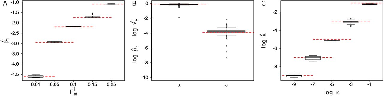
Boxplot of the parameters β1 (left), ν and µ (center) and log(κ) (right). The values are obtained from the mean of the poserior distributions obtained using Flink on the 10 simulations run for each of the set of parameters reported in Table 1. The red otted lines show the true values of the respective parameters.
We next studied the impact of the sample size and the strength of population differentiation on power. In line with findings reported by (Foll and Gaggiotti 2008), power generally increased with , the number of sampled haplotypes and the number of sampled populations (Figure 4A-C). Importantly, larger sample sizes or stronger differentiation was particularly relevant for detecting loci under balancing selection, for which the power was generally lower and virtually zero at low differentiation
  or if only few populations were sampled (J = 2).
Parameters used in simulations

The true positive rate in classifying loci as neutral (black) or under divergent (orange) or balancing selection (blue) as a function of the Fst between populations (A), the number of haplotypes N (B), the number of populations J (C) and the strength of auto-correlation κ (D). Lines indicate the mean and range of true positive rates obtained with Flink (solid) and BayeScan across 10 replicate simulations. Filled dots and the vertical gray line indicate the reference simulation shown in each plot.
We finally compared the power of Flink to that of BayeScan on the same set of simulations. As shown in Figure 4, Flink had a higher power at the same FDR across all simulations, and often considerably so, unless the number of populations sampled was large. If J = 10 populations were sampled, for instance, the power of Flink was about 0.2 higher for loci under divergent selection, and even up to 0.4 higher for those under balancing selection (Figure 4A,B).
Importantly, this increase in power is fully explained by Flink accounting for auto-correlation among the αl values. As shown in Figure 4D, the power of both methods converges as soon as the strength of auto-correlation vanishes (i.e. κ is large). Exploiting information from linked sites to identify divergent or balancing selection can thus strongly increase power, certainly if linkage extends to many loci. This is maybe best illustrated by the much higher power of Flink to identify loci under balancing selection at low differentiation ( , Figure 4A), in which case even many neutral loci are expected to show virtually no difference in allele frequency and only an aggregation of such loci can be interpreted as a reliable signal for selection (Foll and Gaggiotti 2008).
Runtime
Thanks to careful optimization, there is little to no overhead of our implementation compared to that of BayeScan. On the reference simulation of 10 4 loci from 10 populations, for instance, Flink took on average 130 minutes on a modern computer if calculations were spread over 4 CPU cores. On the same data, BayeScan took 361 minutes. However, we note that comparing the two implementations is difficult due to many settings that strongly impact run times such as the number of iterations or the use of pilot runs in BayeScan. Without pilot runs, the run time of BayeScan reduced to 182 minutes on average for the default number of iterations (10 5 including burnin). In the same time, Flink runs for close to 10 6 iterations, but also requires more to converge.
But since computation times scale linerly with the number of loci, they remain prohibitively slow for whole genome applications in a single run. However, they computations are easily spread across many computers by analyzing the genome in independent chunks such as for each chromosome or chromosome arm independently. This is justified because 1) linkage does not persist across chromosome boundaries and is usually also weak across the centromere and 2) because our simulations indicate that 10 4 polymorphic loci were sufficient to estimate the hierarchical parameters accurately.
Application to Humans
To illustrate the usefulness of Flink we applied it to SNP data of 46 populations analyzed as part of the Human Genome Diversity Project (HGDP) (Rosenberg N.A. et al. 2002; Rosenberg et al. 2005) and available at https://www.hagsc.org/hgdp/files.html. We then used Plink v1.90 (Chang et al. 2015) to transpose the data into vcf files and used the liftOver tool of the UCSC Genome Browser (James Kent et al. 2002) to convert the coordinates to the human reference GRCh38.
We divided the 46 populations into 6 groups (Table 2) of between 4 and 15 populations each according to genetic landscapes proposed by Peter et al. (2017). We then inferred divergent and balancing selection using the hierarchical version of Flink on all 2 autosomes, but excluded 5 Mb on each side of the centromer and adjacent to the telomeres. The final data set consists in total f 563,589 SNPs. We analyzed each chromosome arm individally with α max = 4.0, s max = 10 and using an MCMC chain with 7 · 10 5 iterations, of which we discarded the first 2 · 10 5 as burnin. Estimates of hierarchical parameters are shown in figure S2 and the locus-specific FDRs qd (l) and qb (l) are shown for all loci, all groups as well as the higher hierarchy in Supplementary Figures S4-S42. All regions identified as potential targets for selection are further detailed in Supplementary Files. As summarized in Table 2, we discovered between 759 and 1,889 and between 433 and 1,735 candidate regions for divergent and balancing selection, respectively, spanning together about 10% of the genome.
Population groups analyzed
Comparison to BayeScan
We first validated our results by running BayeScan on the same data but for each group individually. We then identified divergent regions as continuous sets of SNP markers that passed an FDR threshold of 0.01 or 0.01 for each method and determined the FDR threshold necessary to identify at least one locus within these regions by the other method. As shown in Figure 5A for selected regions among Europeans, the majority of regions identified by BayeScan were replicated by Flink at small FDR thresholds. In contrast, most of the regions identified by Flink were not replicated by BayeScan, in line with a higher statistical power for the former. Visual inspection indeed revealed that for most regions identified by Flink but not BayeScan, the latter also showed a signal of selection at multiple markers, each of which not passing the FDR threshold individually (see Figure 5B for examples). In contrast, sites identified by BayeScan but not Flink usually consisted of a signal at a single site, suggesting many of those are likely false positives (Figure 5C).

(A) The fraction of regions identified as divergent among Europeans by Flink (green) and Bayescan (black) at a false discovery rate (FDR) of 0.01 (solid) and 0.05 (dashed) also identified by the other method at different FDR. (B-D) Example of regions found under divergent selection by Flink (B), BayeScan (C) or both (D). The dashed line represents the FDR threshold of 0.01.
Results were similar for the other groups (Figure S3), but the correspondence between the methods was higher for African group and considerably lower for the American group, likely due to the different patterns of divergence among populations (Figure S2).
Comparison with a recent scan for selective sweeps
Since positive selection might affect a subset of populations only and hence lead to an increase in population differentiation (Nielsen 2005), we compared our outlier regions also to those of a recent scan for positive selection that combined multiple test for selection using a machine learning approach (Sugden et al. 2018). Among the 593 candidate loci reported for the CEU population of the 1000 Genomes Project (1000 Genomes Project Consortium et al. 2015) and overlapping the chromosomal segments studied here, 293 loci (49.4%) fall within a region we identified as under divergent selection either among European populations (154 loci), at the higher hierarchy (132 loci), or both (7 loci).
To test if this overlap exceeds random expectations, we generated 10,000 bootstrapped data sets by randomly sampling the same amount of loci among all those found polymorphic in the 1000 Genome Project CEU samples and within the chromosomal segments studied here. We then determined the overlap with our outlier regions for each data set. On average, 46.6 loci overlapped with our regions identified among European populations or at the higher hierarchy. Importantly, the largest overlap observed among the bootstrapped data set (72 loci) was much smaller than that observed (293 loci, P < 10 −4).
Example: The LCT region
As illustration, we show the FDRs qd (l) and qb (l) for 30 Mb around the LCT gene in Figure 6 for the higher hierarchy as well as the European, Middle Eastern and East Asian group. The LCT gene is a well studied target of positive selection which has acted to increase lactase persistence in several human populations, including Europeans (Nielsen et al. 2007). Lactase persistence varies among Europeans and decreases on a roughly north-south line (Bersaglieri et al. 2004; Leonardi et al. 2012; Burger et al. 2007; Itan et al. 2009), consistent with the signal of divergent selection we detected among European populations (Figure 6). In line with previous findings (e.g. Grossman et al. 2013), we detected a signal of divergent selection among Europeans also in various genes around LCT, most notably in R3HDM1 but also MIR128-1, BXN4 and DARS. In contrasts, we detected no such signal for the other groups.

Signal of selection around the LCT gene on Chromosome 2q. The orange and blue lines indicate the locus-specific FDR for divergent (orange) and balancing (blue) selection, respectively. The black dashed line shows the 1% FDR threshold. A zoom of the highlighted region is shown on the right indicating the position of several genes: R3HDM1 (R3), MIR128-1 (MI), UBXN4 (UB), MCM6 (MC), DARS (DA) and DARS-AS1 (DA1). The entire Chromosome 2q is shown in Supplementary Figure S7.
Discussion
Genome scans are common methods to identifying loci that contribute to local adaptation among populations. Here we extend the particularly powerful method implemented in BayeScan Foll and Gaggiotti (2008) to linked sites.
Accounting for linkage in population genetic methods, while desirable, is often computationally hard. We propose to alleviate this problem by modeling the dependence among linked sites through auto-correlation among hierarchical parameters, rather than the population allele frequencies or haplotypes themselves. In the context of genome scans, this has been previously successfully by classifying each locus as selected or neutral (Boitard et al. 2009; Kern and Haussler 2010). Here, we extend this idea by modeling auto-correlation among the strength of selection acting at individual loci. While ignoring auto-correlation at the genetic level certainly leads to a loss of information, the resulting method remains computationally tractable. And as we show with simulations and an application to human data, the resulting method features much improved statistical power compared to BayeScan, a similar method that ignores linkage completely.
Accounting for partial linkage particularly improved the power to identify loci with more similar allele frequencies among populations than expected by the genome-wide divergence. These loci are generally interpreted as being under balancing selection Foll and Gaggiotti (2008); Beaumont and Balding (2004), but may also be the result of purifying selection restricting alleles from reaching high allele frequencies. Given the large number of loci we inferred in this class from the HGDP data (about 5% of the genome), we speculate that balancing selection in unlikely the main driver, and caution against over-interpreting these results. But we note that the empirical false discovery rate for loci under balancing selection was extremely low in our simulations.
An obvious draw-back of modeling the locus-specific selection coefficients as a discrete Markov Chain is that for most candidate regions we detected, multiple loci showed a strong signal of selection, making it difficult to identify the causal variant. However, once a region is identified, estimates of selections coefficients can be obtained for each locus individually to identify the locus with the strongest signal, for which one might then also use complementary methods.
We finally note that the implementation provided through Flink allows to group populations hierarchically. Accounting for multiple hierarchies was previously shown to reduce the number of false positives in FST based genome scans (Excoffier et al. 2009) and also applied in an F-model setting (Foll et al. 2014). Aside from accounting for structure more accurately, a hierarchical implementation also allows for genome-wide association studies (GWAS) with population samples. In such a setting, each sampling location would constitute a “group” of, say, two “populations”, one for each phenotype (e.g. cases and controls). The parameters at the higher hierarchy will then accurately describe population structure and loci associated with the phenotype will be identified as those highly divergent between the two “populations”. A natural assumption would then be that the locus-specific coefficients αl are be shared among all groups, i.e. that they are governed by a single HMM. While we have not made use of such a setting here, we note that it is readily available as an option in Flink.
Acknowledgments
This study was supported by two Swiss National Foundation grants to DW with numbers 31003A_149920 and 31003A_173062.
Footnotes
↵1 Department of Biology, University of Fribourg, Chemin du Musée 10, 1200 Fribourg, Switzerland, daniel.wegmann{at}unifr.ch
↵2 Where authors are identified as personnel of the International Agency for Research on Cancer / World Health Organization, the authors alone are responsible for the views expressed in this article and they do not necessarily represent the decisions, policy or views of the International Agency for Research on Cancer / World Health Organization.


