

Abstract
Genes are regulated through enhancer sequences, in which transcription factor binding motifs and their specific arrangements (syntax) form a cis-regulatory code. To understand the relationship between motif syntax and transcription factor binding, we train a deep learning model that uses DNA sequence to predict base-resolution binding profiles of four pluripotency transcription factors Oct4, Sox2, Nanog, and Klf4. We interpret the model to accurately map hundreds of thousands of motifs in the genome, learn novel motif representations and identify rules by which motifs and syntax influence transcription factor binding. We find that instances of strict motif spacing are largely due to retrotransposons, but that soft motif syntax influences motif interactions at protein and nucleosome range. Most strikingly, Nanog binding is driven by motifs with a strong preference for ∼10.5 bp spacings corresponding to helical periodicity. Interpreting deep learning models applied to high-resolution binding data is a powerful and versatile approach to uncover the motifs and syntax of cis-regulatory sequences.
Introduction
Understanding the cis-regulatory code of the genome is vital for understanding when and where genes are expressed during embryonic development, in adult tissues, and during disease. Despite extensive molecular efforts to map millions of putative enhancers in a wide variety of cell types and tissues (1–3), the cis-regulatory information contained in these enhancer sequences remains poorly understood. Enhancers contain arrangements of short sequence motifs that are bound by sequence-specific transcription factors (TFs). While the combination of TF binding motifs is known to be important for the cis-regulatory code, the rules by which the motifs’ syntax influences TF binding and enhancer activity remain more elusive. A widely accepted element of syntax are composite motifs, which consist of two or more strictly spaced motifs that provide a platform for DNA-mediated cooperativity between the corresponding TFs (4). However, whether less strict (“soft”) motif spacing preferences exist and influence the cooperative binding of TFs is not clear.
Experimental manipulations of enhancer sequences, such as mutations or synthetic designs, have repeatedly pointed to the importance of syntax for enhancer function, including soft spacing preferences between motifs (e.g. 5–12)). However, preferred motif syntax derived from such studies are usually not statistically over-represented in genome-wide analyses, questioning whether such rules are generally relevant and impose evolutionarily constraints on enhancer function (13–17). Likewise, unbiased genome-wide surveys for over-represented motif spacing have been conflicting. When patterns are discovered (18–24), they are difficult to validate experimentally and their significance, as well as mechanistic underpinnings, are poorly defined. For example, over-represented instances of strict motif spacings are sometimes associated with retrotransposons that contain multiple TF binding motifs (19, 20). Thus, the appearance of syntax may be the result of biases inherent to genome composition, rather than the result of strong constraints on enhancer function.
The technical limitations associated with identifying genome-wide enhancer syntax could be overcome in two ways. First, by mapping all relevant motifs bound by TFs in vivo with more precision, the statistical power to detect soft motif preferences could be substantially improved. Traditionally, TF binding sites have been mapped in vivo using chromatin immunoprecipitation experiments coupled to sequencing (ChIP-seq). However, the number of confidently mapped binding sites is relatively small due to the limited resolution of the method and the inherent limitations of using position weight matrix (PWM) representations to identify the bound motif instances (25). Second, having an experimental readout for the effect of motif syntax would provide confidence in the functional importance of specific motif spacings. While motif syntax could affect the activity of enhancers through numerous and complex mechanisms, the simplest readout would be to directly detect in vivo cooperative binding of TFs to their motifs.
Both solutions to improving the study of motif syntax can be implemented with ChIP-exo assays such as ChIP-nexus. These in vivo binding assays have near base-resolution due to an exonuclease digestion step during ChIP, (26, 27) which generates precise DNA binding footprints of TFs in vivo (26, 27). This yields more specific TF binding motifs and higher resolution maps of motif instances (27, 28). In addition, the binding profiles uncover distinct patterns associated with indirectly bound TFs (28, 29) or cooperating TFs, in which one TF helps the binding of a second TF on a nearby motif (30). Although the full extent of TF cooperativity at the level of binding is not known, these results suggest that ChIP-nexus may identify TF cooperativity dependent on motif syntax.
Extracting rules of TF cooperativity from ChIP-nexus data is however a challenging computational task. Traditionally, motif discovery (31–34) is performed separately, after identifying bound regions from ChIP-seq data using peak-calling methods that search for generic binding footprints (35–40). To avoid information loss between the two steps, integrative approaches learn the sequence motifs together with their characteristic footprints (19, 28). While this leads to considerable improvements in the detection of directly and indirectly bound motifs, such approaches rely on strong modeling assumptions and do not model the role of motif syntax on TF occupancy.
Here, we develop novel convolutional neural networks (CNNs) and model interpretation techniques to decipher the cis-regulatory code of in vivo transcription factor binding from ChIP-nexus data. Instead of making explicit assumptions about binding patterns and the underlying DNA sequence features, we take advantage of the power of CNNs to learn arbitrarily complex patterns from regulatory DNA sequence that are predictive of base resolution TF binding profiles. CNNs have been shown to accurately predict diverse molecular phenotypes including TF binding from DNA sequence, by fitting flexible mathematical functions composed of hierarchical layers of non-linear transformations of DNA sequence that capture sequence motifs and their higher-order organizational context (41–44).
Although the predictive power of CNNs is undisputed and still improving (45), the challenge is to extract the rules by which motif combinations and syntax predict the in vivo transcription factor binding profiles. While interpretation tools are becoming available to identify predictive sequence features in individual DNA sequences from trained models (41, 42, 44, 46–49), tools for extracting higher-order predictive patterns from sequence predictions are largely lacking (50). Another challenge is that binding data are currently modeled with limited resolution, either as binary binding events (41–43) or as low-resolution, continuous binding signal averaged across 100-200 bp windows (51). The resulting loss of information likely restricts the ability of the CNNs to detect and predict more subtle patterns in high-resolution ChIP-nexus data.
To maximize the potential for identifying motif combinations and the role of motif syntax in ChIP-nexus data, we therefore designed a novel CNN called BPNet that predicts ChIP-nexus profiles at base resolution. We expanded model interpretation methods to enable de novo inference of predictive motif instances in individual regulatory sequences and derive novel motif representations to capture globally predictive sequence features across all binding sites. We further developed new approaches that uses the trained BPNet model as an in silico oracle to infer motif syntax and derive rules of TF cooperativity.
We used BPNet to investigate the motif syntax of the four pluripotency TFs Oct4, Sox2, Nanog, and Klf4 in mouse embryonic stem cells (ESCs). These TFs are important for reprogramming and maintaining cells in a naive pluripotent state, which allows differentiation into any cell type. Due to the importance of the model system, there is ample experimental information to assess the biological relevance of our extracted information.
We discovered known and novel motifs predicted to contribute to the binding of the four TFs, and mapped over 241,000 motif instances in the genome, outperforming current methods in accuracy and resolution. Novel motif representations derived from the model distinguish TF binding motifs from retrotransposons, allowing us to better identify preferred motif syntax. Importantly, we directly extract specific rules of cooperative TF binding from the model. These rules are consistent with the preferential soft motif syntax in the genome and are in remarkable agreement with experimentally characterized protein-protein or nucleosome interactions in ESCs. Furthermore, we observed unexpected rules of TF binding cooperativity, including a broad preference for Nanog to bind DNA with helical periodicity. These results suggest that motif syntax drives TF cooperativity, and that we have developed a powerful and versatile method to identify the rules by which this occurs. Using interpretable deep learning on high-resolution regulatory genomics data paves the way for the systematic discovery of cis-regulatory motifs and syntax in experimentally accessible cell types.
Results
BPNet predicts base-resolution ChIP-nexus TF binding profiles from DNA sequence in mouse ESCs
To obtain genome-wide strand-specific base-resolution footprints for Oct4, Sox2, Nanog and Klf4, we performed ChIP-nexus experiments for each TF in mouse ESCs (Figure 1A). The profiles had higher resolution and specificity compared to ChIP-seq, as we have shown for other TFs with this approach (27). For example, Oct4 and Sox2 are known to form heterodimers on the composite Oct4-Sox2 motif in ESCs (52), and both the Oct4 and Sox2 ChIP-nexus data show sharp, narrow footprints on this motif, while the average ChIP-seq profile is broad (Figure 1B). On the Sox2 motif, only Sox2 but not Oct4 ChIP-nexus data show a strong, sharp footprint (Figure 1B). This motif specificity is not present in the ChIP-seq data, which show binding signal for both Oct4 and Sox2 at the Sox2 motif (Figure 1B). Having confirmed the high quality of the data, we selected a total of 147,974 genomic regions with strong ChIP-nexus signal for Oct4, Sox2, Nanog or Klf4 and sized these regions to 1 kb length.

A) ChIP-nexus experiments were performed on four transcription factors (Oct4, Sox2, Nanog and Klf4) in mouse embryonic stem cells (ESCs). After digestion of the 5’ DNA ends with lambda exonuclease, stop sites are mapped to the genome at single-base resolution. Bound sites exhibit a distinct footprint of aligned reads, where the positive strand peak occurs many bases before the negative strand peak. B) The average ChIP signal at the top 500 Oct4-Sox2 and Sox2 motif sites for Oct4 and Sox2 are shown for ChIP-nexus data (line for positive and negative strand) and ChIP-seq data (grey). Note that the ChIP-nexus data have higher resolution and show less unspecific binding of Oct4 to the Sox2 motif. C) A convolutional neural network (BPNet) is trained to predict the number of aligned reads from ChIP-nexus for all TFs simultaneously at each nucleotide position from 1kb DNA sequence for each strand. D) Observed and predicted ChIP-nexus read coverage of the forward strand (dark) and the reverse strand (light) for the Lefty enhancer located on the held-out test chromosome 8. E) BPNet predicts the positions of local maxima with high signal (around footprints) in the profiles at replicate-level accuracy as measured by the area under precision-recall curve (auPRC) at multiple resolutions (from 1 bp to 10 bp) in held-out test chromosomes 1, 8 and 9 (Methods). F) More convolutional layers (x-axis) increase the number of input bases considered for profile prediction at each position (receptive field) and thereby yield increasingly more accurate profile shape predictions on the tuning chromosomes 2-4 (measured in auPRC as above).
To learn the relationship between DNA sequence and ChIP-nexus binding profiles in these 1 kb regions, we developed a deep convolutional neural network, BPNet, that predicts the ChIP-nexus read coverage profiles at base resolution from the underlying 1 kb sequences (Figure 1C). For these sequence-to-profile predictions, BPNet uses multiple layers of convolutional filters with dilation (51, 53) and residual connections (54, 55) in order to learn increasingly complex predictive sequence patterns in a compositional manner. Therefore, the ChIP-nexus profile predictions are not just based on motifs directly underlying the footprints, but in fact incorporate sequence information from the entire 1 kb sequence. To increase the potential of capturing how multiple motifs and their syntax influence binding of all four TFs, BPNet was jointly trained on ChIP-nexus profiles of all four TFs using multi-task learning. To capture different aspects of the ChIP-nexus data that are interdependent. BPNet uses a multi-scale loss function to learn to map each 1 kb sequence to multiple outputs: the total read counts in the 1 kb region (count prediction), and the positional distribution of read counts across all bases on the + and – strand (profile prediction). This approach allows us to disentangle the influence of sequence features on the total occupancy and on the shape of ChIP-nexus profiles (Methods). Finally, to control for potential biases in the ChIP-nexus profiles, BPNet also models experimental control data (PAtCh-CAP data (49), see Methods).
After training and tuning the models on a subset of the 147,974 genomic regions with strong ChIP-nexus signal from separate sets of chromosomes (called training and tuning sets), genomic regions from the remaining held-out set of chromosomes (called the test set) were used for performance evaluation (Methods). At individual enhancers such as those associated with Lefty1 (56), Zfp281 (57), and Sall1 (58, 59) genes (Figure 1D and Figure S1C), the predicted and observed ChIP-nexus profiles were noticeably similar with highly concordant summits of footprints. Across all regions in the test set, the positions of high predicted versus observed ChIP-nexus counts were also highly concordant (Figure 1E, Methods). The positional concordance was on par with replicate experiments and substantially better than randomized profiles or average profiles at resolutions ranging from 1-10 bp.

A) Observed and predicted ChIP-nexus read counts mapping to the forward strand (dark) and the reverse strand (light) for the Zfp281 and Sall1 enhancers located on the held-out (test) chromosome 1. B) Observed and predicted total read counts for BPNet (top) and replicate experiments (bottom) across the four studied TFs along with the Spearman correlation coefficient. C) auPRC of profile predictions is high across various learning rates on the tuning set chromosomes 2-4 demonstrating the robustness of the model. D) The deconvolutional layer slightly improves the profile predictive performance compared to a point-wise convolutional layer (deconvolution size=1). D) auPRC of profile predictions (top) and the Spearman correlation of total count predictions (bottom) for a range of different relative total count weight α in the BPNet loss function parameterized as λ = α/2 n_obs. Relative weight of 1 (center) denotes equal weighting of the counts and profile loss functions. The best performance is obtained for alpha < 1 showing that putting more weight to profile predictions helps for both profile and count predictions.
Systematic analysis of the network architecture revealed that a key component for reaching high prediction performance was the increased depth of the network (larger number of layers), which determines the total span of local sequence used by the model to predict ChIP-nexus read coverage at any single position (Figure 1F, Figure S1). Nanog was particularly sensitive to network depth, indicating that the learned sequence patterns required to predict Nanog ChIP-nexus profiles span over larger sequence regions (45). In addition, we improved profile prediction performance by prioritizing (up weighting) the profile predictions compared to the total count predictions during training. Irrespective of the relative up weighting, the correlation of predicted and observed total read counts always remained lower than the correlation of total counts between replicates (BPNet Rs = 0.62 vs. replicate Rs=0.94) (Figure S1). These results indicate that while local sequence context (1 kb) is sufficient to accurately capture the shape of ChIP-nexus profiles and positions of binding footprints, longer sequences or other measurements such as local chromatin state may be required to better predict TF occupancy (45). Hence, we performed model interpretation using the profile predictions in downstream analyses. Altogether, our results show that ChIP-nexus profiles can be accurately predicted from local sequences by BPNet.
A suite of model interpretation tools identifies TF binding motifs and maps genomic motif instances with high accuracy
Having learned an accurate sequence model of ChIP-nexus binding profiles of all four TFs, we then investigated whether we could extract predictive sequence patterns such as motifs from the trained model. We previously developed an efficient method called DeepLIFT that can quantify the contribution of each base pair in the input sequence to a single predicted output of a neural network model (60). Since BPNet predicts the ChIP-nexus data at multiple positions, we adapted DeepLIFT to compute base-resolution contribution scores from the entire predicted ChIP-nexus profile across both strands (Figure 2A, Methods). These profile contribution scores are computed in a TF-specific fashion, such that the same sequence will have different contribution scores depending on the TF.

A) DeepLIFT recursively decomposes the predicted binding output of the model for a specific TF for an input DNA sequence in terms of quantitative contribution or importance scores of each base (called the profile contribution score) in the input DNA sequence by backtracking the prediction through the network. B) Procedure for inferring and mapping predictive motif instances using a known distal Oct4 enhancer (chr17:35504453-35504603) as an example. From the predicted ChIP-nexus profile for each TF (top), DeepLIFT derives profile contribution scores that highlight the important bases for the binding of each TF (middle). Regions with high contribution scores (called seqlets) resemble TF binding motifs. TF-MoDISco learns motifs by consolidating similar seqlets across all sequences bound by the TF, which then allows systematic annotation of all predictive instances in the genome to a set of motifs (bottom). C) An outline of the motif discovery and annotation method: TF-MoDISco first scans for seqlets, extends the seqlets to 70 bp, computes pairwise distances between extended seqlets after pairwise alignment and then clusters seqlets to obtain motifs. Each motif is summarized by the contribution weight matrix (CWM) obtained by averaging the contribution scores of each of the 4 bases at each position across all aligned seqlets in a cluster. The corresponding position frequency matrix (PFM) is obtained by computing the frequency of bases at each position. Motif instances are identified and refined by scanning the CWM for each motif for high scoring matches across the profile of contribution scores along candidate sequences genome-wide. D) Number of motif instances found in the ∼150,000 thousand genomic regions for the main short motifs as listed in Figure 4. E) Histogram of the number of mapped motif instances found per region. F) Comparison of the motifs obtained by BPNet-facilitated CWM scanning and classical PWM scanning. The quality of the motif instances for each TF is assessed by determining the Spearman rank correlation of the motif scores with the ChIP-nexus profile heights (Methods and Supplementary material – method comparison).
We illustrate the nature of the DeepLIFT base-resolution contribution scores for each of the four TFs using the Oct4 distal enhancer as an example (Figure 2B). All four TFs show strong predicted footprints matching the observed ChIP-nexus footprints (Figure 2B top, Figure S2A), and TF-specific local subsequences with high contribution scores. Intriguingly, these local subsequences, which we call seqlets, resemble known TF binding sequence motifs (Figure 2B middle).

A) Observed and predicted ChIP-nexus read counts for the Oct4 distal enhancer. B,C,D) Previously validated binding motifs for Oct4-Sox2 were re-discovered by BPNet. ChIP-nexus read counts and BPNet contribution scores for three enhancers are shown. B) The Oct4-Sox2 motif site in the Klf4 E2 enhancer was validated by deleting the site using CRISPR/Cas9 (69). C,D) The Oct4-Sox2 binding motifs in the Nanog and Fbx15 enhancers were confirmed previously using reporter assays of constructs with various motif mutations (70, 71).
One of the most prominent seqlets matches the composite Oct4-Sox2 motif (TGCATNACAA), which has previously been mapped to this exact position in the Oct4 enhancer (61). We note that this motif has high contribution scores for not only Oct4 and Sox2, which are directly bound to the motif, but also for Nanog and Klf4 at slightly lower levels (Figure 2B middle). This suggests that the Oct4-Sox2 motif is indirectly important for the binding of other TFs. The known Klf4 motif (CGCCCC) was also detected as an important seqlet and it was specific for Klf4 binding. Other seqlets were not as readily identifiable as matches to known motifs. For example, it was unclear whether a short TGAT sequence in the middle of the Nanog footprint (position ∼100) is a Nanog motif since previous reports on its consensus have been conflicting (62–68). This demonstrates the ability of contribution scores to highlight TF binding motifs, but also indicates the need to identify and characterize the motifs more systematically.
To systematically summarize recurring predictive sequence patterns across all binding sites, we used TF-MoDISco, an algorithm we recently developed for de novo motif discovery from contribution scores (48). For each TF, TF-MoDISCo automatically identifies seqlets across all its putative bound regions and then clusters optimally aligned seqlets based on pairwise similarity scores (Figure 2C). TF-MoDISCo then derives for each cluster a novel motif representation called a contribution weight matrix (CWM) by averaging the contribution scores of each of the four possible bases at each position across all aligned seqlets in the cluster (Figure 2C). TF-MoDISco also derives a position frequency matrix (PFM), which contains the base frequencies instead of the average contribution scores (Figure 2C). By normalizing the PFM by nucleotide background frequencies, we further derive a classical log-odds position weight matrix (PWM) for each motif, which we use for comparisons with PWM motifs derived by other methods.
In total, TF-MoDISCo detected 145,748 seqlets across the 147,974 genomic regions and clustered them into 51 motifs. We were able to interpret all 51 motifs, but due to retrotransposons (see Figure 3 below) and subtle differences between subsets of similar motifs, we focused on 11 representative TF binding motifs for further analysis (Methods, Figure S3). They include the well-known Oct4-Sox2, Sox2, and Klf4 motifs, as well as known and novel motifs for Nanog and other pluripotency TFs that we did not profile, including Zic3 and Essrb (Figure S3 and see Figure 4 below).

A) All 33 short motifs (information content < 30 bit) are shown with (from left to right): motif ID, number of seqlets supporting the motif, CWM, PFM, and average ChIP-nexus read count distribution (footprint) for each TF. All sequence logos and profile plots share the same y-axis in each column. Motif ID consists of the TF name for which the motif was discovered (O for Oct4, S for Sox2, N for Nanog, and K for Klf4) and the order in which the motif was discovered by TF-MoDISco run for each TF. B) Motifs clustered according to their similarity using hierarchical clustering. The 11 representative motifs selected manually are shown on the left.

A) In addition to the Oct4 and Sox2 motif, the strictly-spaced Oct4-Sox2 motif was identified by TF-MoDISco separately (left). The CWM of the Oct4-Sox2 motif correlates with the structure of Oct1 and Sox2 bound to the Oct4-Sox2 motif (right). For visualization, amino acids of Oct1 and Sox2 that contact DNA are shown as solid, and the atoms in the DNA bases are shown as spheres colored by base are sized according to the contribution scores shown in the CWM below (right). B) Example of a retrotransposon (RLTR9E N6) that results in a composite motif with strict spacings between a Sox2, Nanog and Klf4 binding site. The PFM is shown on top and the CWM for each TF is shown below, highlighting the sequences that contribute to binding. C) The long motifs (green) are predominantly annotated as repeat elements. D) Histogram of the information content (IC, in bits) of PFMs of all motifs obtained from TF-Modisco shows a bimodal distribution. Motifs with an IC <30 were classified as short motifs (grey), and those with >30 as long motifs (green). E) Overview of all long motifs with their respective ID, motif information content (PFM), number of CWM instances in genomic regions, fraction of motif instances overlapping with a repeat, and the most frequent RepeatMasker annotation. Highlighted are potential locations of the four main motifs (Oct4-Sox2, Sox2, Nanog and Klf4) within the repeat elements. F) Sequence composition of individual instances of the RLTR9E N6 motif in the genome were sorted by the number of substitutions (Kimura distance) from the consensus motif (B) such that the most ancestral sequences are at the top. Keeping these sequences in the same order suggests that the Nanog, Sox2 and Klf4 ChIP-nexus binding footprints (right) are already present in the ancestral sequences and that the spacing between them is largely constant across all sequences. G) Analysis of the most frequent quartile of genome-wide shows that the top motif pairs come from ERV retrotransposons. Note that since motif centers are defined as the center of the trimmed motif, the absolute distance between two motifs is not exactly defined.

A) The discovered short motifs contain known motifs, new motifs (***), and known motifs new in this context (*). From left to right: motif ID, motif name, CWM, PFM. All sequence logos share the same y-axis. B) The highest average contribution score of the motif across TFs may indicate direct binding C) The TF’s average ChIP-nexus footprint (read count distribution on the positive strand at the top and negative strand at the bottom) indicates whether the motif is directly bound (sharp profile, marked with grey background), indirectly bound (fuzzy profile) or not bound at all. The footprints for each TF share the same y-axis. D) Sharp Nanog binding was associated with three Nanog motif variants (shown as CWM), which show the strongest ChIP-nexus footprint at the TCA sequence (blue). The CWM of Nanog-mix (N5) and Nanog-alt (N4) contain a sequence that matches the sequence AATGGGC bound by Nanog in a crystal structure (grey) (81). The CWM of Nanog-alt contains GG (pink). E) tRNA-overlapping B-box motif instances were reoriented to match tRNA gene transcriptional direction and sorted by tRNA gene start proximity. This reveals Oct4 binding across both the B-box and tRNA gene start/stop sites. F) The B-box motif is bound by Oct4 at 283 tRNA genes with a diverse set of amino acid classifications. H) Model representing the relationship between the B-box motif to tRNA genes and Oct4.
Using these 11 representative TF motifs, we next set out to comprehensively map predictive motif instances in all genomic regions by rescanning the contribution scores for motif matches (scheme in Figure 2C, results for Oct4 enhancer in Figure 2B). A motif instance was called a match to a CWM if it had a high contribution score and was similar to the CWM (Methods). In total, we obtained 241,005 unique motif instances in the 147,974 genomic regions, with Klf4 motifs occurring most frequently (Figure 2D). Altogether, 72,696 regions (48.1%) have at least three predictive motif instances and 20,352 regions (13.5%) have at least 5 predictive motif instances (Figure 2E). In support of the map’s accuracy, motif instances that are supported by previous independent validation experiments were rediscovered. For example, we identified the Oct4-Sox2 binding site of the Klf4 E2 enhancer (Figure S2B), which was functionally validated by CRISPR/Cas9 (69), and the Oct4-Sox2 binding sites in the Nanog and Fbx15 enhancers (Figure S2C,D), which were validated in reporter assays by small deletions (70, 71).
Next, we compared the CWM based motif instances in our map to those obtained by the traditional approach of scanning the raw DNA sequence with PWM representations of the same motifs. To evaluate the motif instances, we measured the ChIP-nexus signal strength in their immediate vicinity. Since our motif instances are derived from BPNet’s predicted CWMs and contribution scores, we performed this comparison only on sequences from the held-out (test) chromosomes, which were not used to train BPNet. Thus, the motif instances obtained by our CWM scanning method were derived from BPNet’s predictions considering the entire 1 kb input sequence, without having been explicitly trained on the corresponding ChIP-nexus data. We found that the motif instances from CWM scanning were substantially more strongly correlated with local ChIP-nexus signal strength than those from PWM scanning (Figure 2G). This was true for all TFs, with the most striking improvement observed for Nanog, which binds a very short motif (Rs = 0.36 for CWM versus 0.06 for PWM, Figure 2G). This strong difference was not due to the poor quality of our PWMs since PWMs obtained from applying ChExMix to our ChIP-nexus data were almost identical to PWMs obtained from TF-MoDISco (Supplemental Material: Method comparison). Instead, this strong difference is likely due to the much higher false-positive rate of PWM scanning compared to CWM scanning (Supplemental Material: Method comparison). These results highlight the advantages of using profile contribution scores and the novel CWM motif representation to identify motif instances associated with ChIP-nexus footprints.
Retrotransposons bound by multiple TFs confound the interpretation of strict motif syntax
Unlike conventional motif discovery methods which typically learn relatively short (4-25 bp) ungapped motifs, TF-MoDISCo has the ability to discover long (<70 bp), more complex motifs. This is beneficial since it allows TF-MoDISCo to discover predictive motifs that are found frequently with an exact base pair spacings between each other, a feature often used to identify motif syntax. Indeed, TF-MoDISCo discovered the composite Oct4-Sox2 motif (Figure 3A). Based on modeling Oct1-Sox2, the specific spacing in the Oct4-Sox2 motif promotes the cooperative binding of Oct4 and Sox2 through protein-protein interactions and DNA-mediated allostery (52, 72, 73). The specific DNA contacts made by the heterodimer correspond to the bases with high contribution scores in the Oct4-Sox2 CWM (Figure 3A right).
In contrast to the Oct4-Sox2 motif, the less well-studied composite Sox2-Nanog motif identified using SELEX (67) was not discovered by TF-MoDISCo. Consistent with this result, we found no evidence that this motif was bound in our ChIP-nexus data (Figure S4A). Instead, our data suggest that the cooperative binding between Sox2 and Nanog occurs through a different mechanism, one that does not involve a composite motif (see below).

A) No evidence for binding to the previously reported Nanog-Sox heterodimer motif. Median ChIP-nexus signal, predicted BPNet signal, and DeepLIFT contribution of Oct4, Sox2, Nanog, and Klf4 across motif instances containing TF-MoDISco Oct4-Sox2, Sox2, Nanog, and Klf4 motifs and the putative Nanog-Sox heterodimer motif (RMWMAATWNCATTSW) (67). B) Histograms depicting the frequency of center-to-center motif pair spacings across the 11 representative motifs. Colors represent ERV classes which overlap with the corresponding motif pairs.
Among the 51 motifs, we found additional composite motifs in which the CWMs captured multiple TF binding sites with fixed spacing constraints (Figure 3B). However, the PFMs of these motifs were unusually long (> 40 bp) with very high information content. This implies that the genomic instances of these composite motifs shared near identical base composition across the entire length of the pattern, including the parts of the sequence that do not have significant contribution scores to TF binding. We therefore tested whether the genomic instances (which are uniquely mappable based on the ChIP-nexus read lengths) of the long composite motifs overlapped with repeat elements, sequences that get copied and inserted at multiple loci throughout the genome. Among the 18 long composite motifs that have high information content (30-100 bits) (Figure 3C), the majority (>80%) of motif instances overlapped with repeat elements as annotated by Repeat Masker (Figure 3D). Most of these repeats were classified as long-terminal repeats (LTRs) of endogenous retrotransposon viruses (ERVs), and included the ERVK, ERVL and the ERVL-MaLR family (Figure 3E). These results suggest that composite patterns with strict motif spacings are frequently due to retrotransposons bound by these TFs.
This idea is consistent with previous observations that retrotransposons in ESCs may contain multiple TF binding sites and previous suggestions that multiple functional TF binding sites may have already been present in an ancestral ERV copy before replicating in the genome (74–78). In support of this, we found that the motif instances with the least number of mutations, which likely represent the most recently integrated ERVs, were already bound by multiple TFs (Figure 3F).
These results suggest that frequently observed strict motif spacing can be the result of spreading retrotransposons, rather than functional constraints. To test the prevalence of this confounding effect, we analyzed to what extent over-represented strict motif spacings are due to retrotransposons. For this, we selected motif pairs with a minimum number (>500) of co-occurring motif instances in our regions and determined the relative frequencies of the distances for each motif pair. Among the top 1% highest frequencies from all motif pairs, 83% were annotated as ERVs, including ERVK, ERV1, ERVL and ERVL-MaLR (Figure 3G, Figure S4B). Notably, the top most frequent distances were all larger than 20 bp (Figure 3G), thus exceeding the typical distance between motifs found in composite motifs that promote TF cooperativity (79, 80). This makes it unlikely that these over-represented strictly spaced motif instances represent functional constraints on motif syntax.
ChIP-nexus profiles reveal direct and indirect binding at discovered motifs
Rather than analyzing motif spacings, we next analyzed whether the 11 representative TF motifs might mediate cooperative binding (Figure 4A). Such cooperative binding could allow us to directly measure an effect of motif syntax. We noticed that many motifs had high average contribution scores for multiple TFs (Figure 4B). Moreover, we discovered motifs of pluripotency TFs that we did not profile, including the Zic3 and Essrb motifs (Figure 4A), which we validated with additional ChIP-nexus experiments (Figure S5A,B). Thus, BPNet predicts that Oct4, Sox2, Nanog, and Klf4 frequently bind cooperatively, with the help of motifs from other TFs.
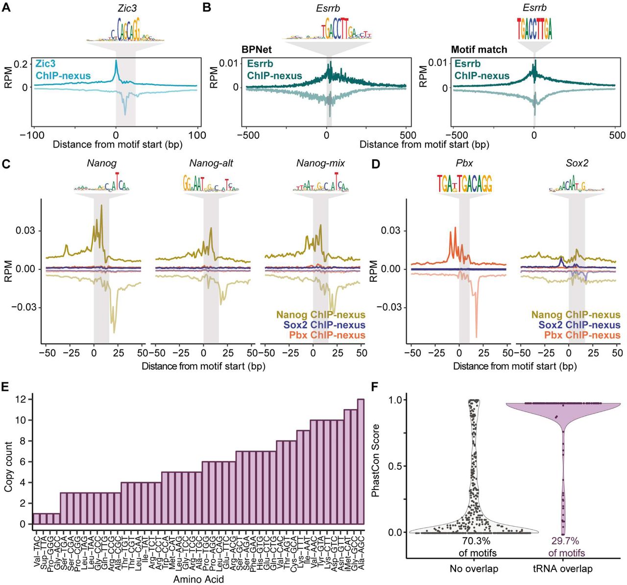
A) Validation of the discovered Zic3 motif. B) Validation of the discovered Essrb motif. Averaged Esrrb ChIP-nexus footprints centered across the TF-MoDISco Esrrb motif and the top 1000 motif-matched Esrrb motif (TCAAGGTCA) regions. C) Nanog validation: Averaged Nanog, Sox2, and Pbx ChIP-nexus footprints centered across the three TF-MoDISco Nanog motifs. D) Average Nanog, Sox2, and Pbx ChIP-nexus footprints at the TF-MoDISco Sox2 motif shows that Pbx and Nanog do not bind specifically. Average Nanog, Sox2, and Pbx ChIP-nexus footprints at the top 5000 scoring sites containing the Pbx motif (TGAKTGACAGG) show that Sox2 and Nanog are not bound to these sites. E) The average phastCon scores (phastCons60way.UCSC.mm10) across the B-box that do and do not overlap with genomic tRNA database (GtRNAdb) annotated tRNAs (141). F) Copy counts of tRNAs overlapping with the B-box, separated by amino acid anti-codons.
One explanation for the contribution of additional motifs is indirect binding through a partner TF, or “tethering”, which has been observed with low-resolution ChIP data (16, 20, 66, 82, 83) and ChIP-exo data (28, 29). Using the learned motifs that matched the known Oct4-Sox2, Sox2, and Klf4 motifs as benchmarks, we found that directly bound motifs show very sharp average ChIP-nexus footprints for the corresponding TF (marked in grey in Figure 4C). In addition, we observed broader, more fuzzy footprints, which we attribute to indirect binding. Their level of occupancy correlates well with the contribution scores of the motif for the indirectly bound TF (Figure 4B,C), suggesting that the indirect footprints are predicted by BPNet.
The property of ChIP-nexus footprints to distinguish direct from indirect binding helped us identify and characterize some of the less well-described motifs. Most notably, we identified Nanog motifs that have a sharp Nanog footprint: Nanog, Nanog-alt and Nanog-mix, the latter of which is partially redundant with the first two (Figure 4D). All have a main footprint around a TCA core sequence, which closely resembles the Nanog motif identified previously by a thermodynamic model from ChIP-seq data (68). Consistent with direct binding, a closely matching sequence (GCCATCA) is bound by Nanog in an EMSA gel shift assay (68). Nanog-alt and Nanog-mix also contain the sequence to which monomeric Nanog is bound in a crystal structure (AATGGGC) (81), and Nanog-alt contains an additional GG to the left (Figure 4D). Given these two separate direct DNA contacts, the observed Nanog binding footprint likely represents Nanog binding as a homodimer (84), although the existence of an unknown Nanog binding partner cannot be ruled out (Figure S5C,D).
We also identified additional motifs bound by Oct4: a canonical Oct4 motif that binds monomeric Oct4 (85) and a near-palindromic motif (Oct4-Oct4) that likely binds Oct4 homodimers since it resembles the MORE and PORE motifs (86, 87) (Figure 4A). This motif has not previously been shown to be bound in ESCs in vivo, but is known to be important during neuronal differentiation (88). We also found an additional, longer motif for Klf4 (Klf4-long), which is bound by Klf4 more weakly than the canonical motif (Figure 4A).
An unexpected motif that initially looked like it was directly bound by Oct4 was a long palindromic motif known as the B-box (Figure 4A), which mediates RNA polymerase III transcription (89, 90). The motifs were found inside ∼280 highly conserved tRNA genes with diverse amino acid anti-codons (Figure 4F, Figure S5E,F). Since the B-box motif is palindromic, we computationally oriented the motifs based on the transcription direction. This revealed that Oct4 strongly binds upstream and downstream of the tRNAs, while binding to the B-box with a more fuzzy footprint (Figure 4G,H). Together with previous evidence (91–93), these results suggest that Oct4 binds indirectly to the B-box via TFIIIC and that this binding may be functionally important for tRNA expression in ESCs.
Finally, we analyzed the indirect footprints in more detail. This revealed that indirect tethering frequently appeared to be directional, as reflected both in the average binding footprints and the contribution scores (Figure 4B,C). This effect was prominently observed for Sox2 and Nanog, which have been shown to physically interact with each other and were thought to bind together to a composite motif (67, 94). However, we found that Nanog was bound indirectly to the Sox2 motif, but Sox2 was not bound to the Nanog motif. This suggests that these TFs indeed cooperate, but with a different mechanism than previously envisioned. We therefore set out to analyze more systematically how motif pairs influence cooperative binding, which would represent a means to identifying motif syntax.
Using BPNet like an in silico oracle reveals cooperative TF interactions
We created two in silico tools that allowed us to systematically interrogate BPNet, like an oracle, to predict whether binding of a TF to its motif is enhanced in the presence of a second motif, and how this change in binding depends on the relative spacing between the motifs (Figure 5A,B). The first approach uses synthetically designed sequences (Figure 5A), while the second uses genomic sequences with and without perturbations (Figure 5B). For both approaches, we used the motifs most strongly bound by each of the four TFs, which are the Oct4-Sox2, Sox2, Nanog, and Klf4 motifs, respectively (shown in Figure 4). To ensure maximum specificity of the predicted TF binding signal, we determined the position of the predicted summit of the footprint on each strand and consistently measure the change in binding at this position. We also subtract indirect binding from the footprint’s shoulder to minimize indirect effects (Figure S6A) (Methods).

A) The influence of motif B on the binding of TF A at motif A is quantified by the fold change of predicted profile height at the reference summit position when motif B is present or absent nearby (hAB vs hA). The binding fold change is corrected for the “shoulder” effect of motif B by subtracting the predicted profile height when only motif B is present in the sequence. B) Spacing distribution of all CWM-derived motif instance pairs in the genome stratified by motif identity and strand orientation. Note that for homotypic interactions, ++ and -- are the same and are shown as ++. C) In silico analysis of motif interactions on synthetic sequences measuring the predicted binding fold change for all motif pairs across all strand orientations (Supplementary to Figure 5C).

A) Outline of the in silico analysis on synthetic sequences, which tests whether the binding of TF A at motif A is influenced by the presence of a nearby motif B. First, the motif A is inserted into 128 different background sequences. Next, BPNet is used to predict the average TF binding profile of TF A averaged across all sequences (averaging out randomly created binding effects in the background sequences). The profile summit positions and their magnitude hA are registered as a reference point (top left). Motif B is inserted at a specific distance from motif A into a new set of random sequence and the average predicted profile height at the registered reference summit is measured (hAB). The fold-change of TF binding profiles is used to quantify the interaction between motifs. B) The second type of in silico motif interaction analysis uses genomic sequences containing motif instance pairs as determined by CWM scanning instead of random background sequences with inserted consensus motif sequences to determine hAB. Profile height at motif A for TF A in the absence of motif B (hA) is obtained by replacing the sequence at motif B with random bases and letting BPNet make the profile prediction. C) Examples from the synthetic in silico analysis as outlined in A showing either protein-range interactions involving Nanog and Sox2 (left) or nucleosome-range interactions exerted by the Oct4-Sox2 motif on the binding of Sox2, Nanog or Klf4, respectively (right). Results are shown for the +/+ orientation of the two motifs. D) The genomic in silico mutagenesis analysis uses the average of all motif orientations, and yields similar results as shown in C. E) Quantification of the results shown in D as heat map. The distances < 35 bp is shown as representative for protein-range interactions, while 70-150 bp is shown as representative for nucleosome-range interactions. F) Odds by which two motifs are found within a specified distance from each other divided by the odds the two motifs would be found in the proximity by chance (observed by permuting the region index). * denotes p-value < 10−5 using Pearson’s Chi-squared test (Methods).
In the synthetic approach, predicted binding of the first TF (TF A) is measured on its corresponding motif (motif A) embedded in random DNA sequences. A second motif (motif B) is then added with decreasing distances to the motif A and the resulting fold change in predicted binding of TF A to motif A is measured (B -> A in Figure 5A, Movie S1). The procedure is then repeated by anchoring motif B and measuring the fold change in binding of the second TF (TF B), while adding motif A at decreasing distances (A -> B in Figure 5A). Such an approach is not feasible experimentally since synthetic sequences may harbor cryptic binding motifs for TFs (even after excluding known motifs), and therefore the number of sequences tested would have to be large in order to gain confidence into specific motif interactions. In the in silico approach, however, we can use more than 100,000 random sequences as the synthetic sequence context, thereby averaging out spurious effects.
Using the synthetic approach, we mapped the interactions between all motif pairs. We found no obvious effect of motif orientation, but observed specific and clearly different interaction patterns between motif pairs (Figure S6B,C). For example, the predicted Nanog binding at the Nanog motif was strongly enhanced when another Nanog motif was nearby, but interestingly, this enhancement exhibited a periodic pattern with decreasing distances between the motifs (Figure 5A). A similar periodic enhancement of Nanog binding at a Nanog motif was observed when a Sox2 motif was nearby. This was not true the other way around since Sox2 binding at the Sox2 motif was not enhanced by a Nanog motif. However, Sox2 binding at the Sox2 motif was enhanced in the presence of another Sox2 motif nearby (Figure 5A). Thus, BPNet predicts that Sox2 and Nanog strongly interact and that this interaction is directional, consistent with the indirect footprints we observed. The magnitude of this interaction was strongest at close distances (<35 bp) and decayed rapidly with further distances. Such distance could be bridged by protein-protein interactions, which Sox2 and Nanog have been shown to engage in (67, 94). We therefore refer to this interaction distance as protein-range. We note however that similar distances have been observed for TF interactions mediated by DNA-mediated allostery, which do not rely on specific protein-protein interactions (4, 95).
We also observed interactions at nucleosome distance. In the presence of Oct4-Sox2, the predicted binding of Sox2, Nanog, and to a lesser extent Klf4, was enhanced at distances up to 150 bp, thus in nucleosome range (Figure 5A). Interestingly, Oct4 and Sox2 have been characterized as pioneer TFs, which can bind nucleosomes and make the region more accessible for other TFs (69, 96, 97). Our observed interactions therefore suggest that Oct4-Sox2 is a strong pioneer motif. Consistent with this, these interactions were also directional: the Oct4-Sox2 motif greatly increased the predicted binding of other TFs, while the motifs of the other TFs did not substantially affect the predicted binding of Oct4. These differences in distance and directionality among all interactions can also be summarized as heat map using the distance intervals of <35 bp and 70-150 bp (Figure 5C).
In the genomic in silico approach, we identified all non-overlapping motif instances of the four motifs in the original genomic sequences and measured the fold change in TF binding with and without perturbation of a nearby motif. For each motif pair, we measured TF binding (TF A) to its motif (motif A) before and after replacing a second motif (motif B) with a random sequence (B -> A), and vice versa (A -> B)(Figure 5B, example in Figure S7A). The advantage of this approach is that we can directly compare predicted binding to the experimentally measured in vivo binding data before applying the perturbations.

A) Example genomic in silico mutagenesis analysis at the distal Oct4 enhancer. Predicted ChIP-nexus profiles and the contribution scores greatly decrease at both motifs (Oct4-Sox2 and Nanog) when erasing the Oct4-Sox2 motif (through random sequence insertion). By contrast, when the Nanog motif is erased (right), the predicted profile and the contribution scores of Oct4-Sox2 motif remain intact. B) Such directional effect of motifs can be quantified by the corrected binding fold change (Figure 5B, Figure S5A) for all motif pairs in the genome and visualized as a scatterplot. C) Example scatterplot for the interaction between Sox2 and Nanog. Sox2 shows a positive directional effect on Nanog most profound for short motif distances (<35 bp). D) Predicted binding fold changes for all motif pairs in genomic sequences.
Using this approach, we again observed that most motif pair interactions were directional, rather than mutual (Figure S7B,C,D). Overall, the interaction patterns were very similar to the synthetic approach, albeit of lower magnitude (Figure 5B, Figure S7D). The smaller effect sizes might be due to the imperfect binding motifs present in the genome since the synthetic approach used the best matching sequence for each motif. It is also possible that motif perturbations can be buffered by additional motifs that are present in genomic sequences, but not in the synthetic context.
In summary, both in silico approaches yielded similar results and pointed to two interesting findings. First, we observed protein-range and nucleosome-range interactions by the way the motif interaction strength decayed with increasing distances. Second, we observed a strong directionality in the pairwise interactions between motifs, which suggests a hierarchical enhancer model, in which some TFs preferentially bind first and then assist other TFs in binding to the enhancer.
Having characterized cooperative interactions, we now revisited the motif spacing analysis. To focus on soft preferences for motif spacing, we removed retrotransposons containing strictly spaced motifs and determined which motif pairs co-occur more frequently than expected by chance (Figure 5D, Figure S4B). The Nanog motifs were most strongly overrepresented at short distances to Sox2 and other Nanog motifs (<35 bp), consistent with their protein-range interactions. At intermediate distances (35-70 bp), the Oct4-Sox2, Sox2 and Nanog motifs all preferentially co-occur, while the Klf4 motif only co-occurs more frequently with other Klf4 motifs, consistent with its weaker interaction. At nucleosome-distance (70-150 bp), the Oct4-Sox2 motif still co-occurs with Nanog, consistent with its pioneering role. Strikingly, even though the BPNet model architecture can capture potential motif co-occurrence and interactions up to 1 kb apart, motif pairs exhibit no significant over-representation beyond 150 bp, suggesting that motif interactions that are predictive of TF footprint patterns do not frequently extend beyond a single nucleosome. Taken together, we detected genome-wide soft preferences for motif spacings that correspond to some extent with detected cooperative binding interactions and thus are likely functionally relevant motif syntax.
Nanog binding has a strong ∼10.5-bp periodic pattern
The most remarkable soft motif syntax we observed was associated with the Nanog motifs. The pairwise spacings between genomic Nanog motif instances showed a strong preference for distances of a multiple of ∼10.5 bp in all possible motif orientations (Figure 6A, Figure S4B, Figure S6B). A ∼10.5 bp periodicity is a biophysical property of the DNA helix (98) and had already been observed in the in silico interaction analysis, where BPNet predicted enhanced binding for Nanog in a periodic pattern.

A) The pairwise spacing of all CWM-derived Nanog motif instances in the genome in all possible orientations shows a periodic pattern (++ includes the -- orientation). B,C) Motifs derived by PWM scanning or ChEXMix do not show a pronounced periodicity. D) The CWM, but not the PFM, of the main Nanog motif has periodic nucleotides in the flanks. E) A heat map of the contribution scores of the individual Nanog instances also show this periodic pattern, the average of which is shown below. F) Projection of the preferred Nanog periodicity to the outward facing major grooves of the DNA wrapped around a nucleosome. Average CWM scores from the Nanog motif (red) and the DNA backbone (light blue) are highlighted. Histones H2A, H2B, H3 and H4 are marked in the center. G) A Fourier power spectrum of the average contribution score (after subtracting the smoothed signal) reveals an average periodicity of 10.9±0.6 bp. H) Heterologous motif combinations of Nanog with Sox2, Oct4-Sox2 and Zic3 also show a preferred spacing with the same periodicity. The distance between two motifs is always kept positive by placing the second motif in the pair downstream of the first motif in the pair. All 4 motif orientations are considered: + denotes the motif lies on the forward strand and – denotes the motifs on the reverse strand. I) Nanog ChIP-nexus binding on average is higher when Nanog motifs have the preferred spacing or when another motif such as Sox2 or Oct4-Sox2 is located nearby with the preferred periodic spacing. J) Fraction of the power spectrum with 10.9 bp periodicity for all discovered motifs for different TFs. The periodicity is highest for motifs that contribute to Nanog binding, followed by the motifs contributing to Sox2 binding. Motifs with high periodicity that are not retrotransposons are labeled.
Nanog is a well studied TF and hence it is surprising that the preferential helical spacing of Nanog motifs has been missed. This is most likely because computational methods that use classical PWMs to scan regions for motif instances suffer from high false discovery rates. Consistent with this idea, no obvious helical periodicity was observed when we analyzed the pairwise spacings of the Nanog motif instances identified by PWM scanning (Figure 6B). We also tested whether ChEXMix, a state-of-the-art integrative motif discovery tool for ChIP-exo/nexus data could identify the helical periodicity with the help of our Nanog ChIP-nexus data (Figure 6C). However, even with this approach, the pairwise spacings of Nanog motif instances did not show strong helical periodicity, most likely because ChEXMix cannot easily resolve multiple closely spaced binding motifs (Figure 6C, Supplemental Material: Method comparison). These results illustrate the difficulties in identifying Nanog’s binding specificity in vivo (62–68) and confirm the high accuracy and resolution of the CWM scanning approach.
The helical binding preference of Nanog is however very plausible and of interest since helical phasing has long been thought to be a possible element of the cis-regulatory code. Various experiments have suggested that helical spacing between DNA elements can impact gene expression (99–104), and computational analyses have identified binding motifs spaced with helical periodicity (21, 23). Furthermore, more recent evidence suggests that certain TF classes, such as homeodomain TFs like Nanog, bind to nucleosomes with helical periodicity (23, 105, 106). The scope and high resolution of our data, as well as our results from cooperative interactions, therefore provide a unique opportunity to analyze this binding preference within cis-regulatory regions in more detail.
When we analyzed the CWM of the main Nanog motif at full length (before trimming it to the core sequence), we noticed flanking A/T bases in a periodic pattern (Figure 6D). This pattern is not clear from the corresponding PFM representation, suggesting that these A/T bases are not statistically overrepresented across all motif instances, but when present, contribute strongly to the Nanog binding predictions. The same periodic pattern was also observed in contribution scores profiles of individual Nanog motif instances (heat map in Figure 6E). This suggests that the periodicity observed for Nanog is very broad and can occur in the presence of very weakly contributing bases.
The simplest explanation for the broad binding preference is that Nanog binds nucleosomal DNA, similar to other homeodomain TFs (105, 106). The DNA major groove to which Nanog binds is accessible from the solvent side and contains higher frequencies of A/T bases (81, 107). To capture this binding preference, we calculated the average contribution scores across 200-bp regions centered on the Nanog motif (Figure 6E bottom), and to account for the higher binding at the center, we subtracted its smoothed average. We then projected this profile onto the DNA of a nucleosome structure (Figure 6F). While this is a plausible model for Nanog binding, we noticed that the periodicity was slightly larger than the ∼10 bp average A/T step and the solvent accessibility of the modeled nucleosome (Figure S8). We therefore calculated a Fourier power spectrum to quantify periodic patterns across all possible frequencies. This revealed a strong periodicity pattern averaging around 10.9 bp (+− 0.6 bp) (Figure 6G). This falls within the observed 10-11 bp periodicity of DNA observed in vitro and in vivo (98, 108–111), is similar to the preferential motif spacing of ∼11 bp observed previously (21, 23), and consistent with observations that cis-regularory regions do not contain average nucleosomes (112, 113).

A) The periodicity of the Nanog CWM (blue at top) is similar to (but slightly larger than) the periodicity of the average frequency of dinucleotides AA/AT/TA/TT (AT step) across the nucleosomes in ESCs (orange) (149) and the solvent-accessible surface area (SASA) of the bases in the nucleosome crystal structure (black). SASA and AT step values are centered around the dyad, while the Nanog CWM is positioned 4 bp away from the CWM maximum to align it on the left side of the dyad with SASA and the known preference of Nanog to bind the DNA major groove (81). Since SASA is highest when the major groove faces away from the core histone proteins, Nanog could bind at the solvent-accessible surface of nucleosomes. The AT step, which facilitates contacts with the histone proteins underneath the outward-facing major groove (107), is also in phase with SASA and thus could coincide with the AT-rich sequences that contribute to Nanog binding. B) Normalized power spectra of the three signals in (A) show strong peaks around 10-11 bp, with the Nanog CWM periodicity being on the larger side of the spectrum. These results raise the possibility that nucleosomes bound by Nanog are not (or no longer) average canonical nucleosomes like the one in the crystal structure.
We next asked whether the motifs of partner TFs, which enhanced Nanog binding in the in silico interactions, showed preferred spacings to the Nanog motifs. Remarkably, the pairwise motif spacings of Nanog with either Sox2, Oct4-Sox2 or Zic3 also showed strong helical periodicity regardless of motif orientation (Figure 6H), consistent with Sox2 contacting Nanog through direct protein-protein interactions (67, 94). To obtain further evidence for cooperative binding, we then analyzed average ChIP-nexus Nanog binding at Nanog motifs as a function of distance to Nanog, Sox2 or Oct4-Sox2 motifs. For all motif pairs, the average Nanog footprint was higher at the preferred helical spacing (Figure 6I), which provides a potential explanation for the corresponding motif periodicity learned by BPNet.
We then analyzed to what degree any of the motifs by themselves showed this periodic spacing preference by calculating the fraction of the power spectrum at 10.9 bp for all 51 motifs (Figure 6J). This revealed that the motifs predicted to contribute to Nanog binding have the strongest 10.9 bp periodicity, with the main Nanog motif at the top, followed by the other two Nanog motifs, the Sox2 motif and the Oct4-Sox2 motif (Figure 6J). The motifs important for Sox2 binding also showed some moderate periodicity, while motifs contributing to Oct4 and Klf4 binding had minimal periodicity.
This suggests that helical periodicity is not a universal feature of motif syntax, but a preferred binding feature of some TFs and the respective partner TFs that they cooperate with. Based on previous experimental evidence on the relationship between Oct4, Sox2, Nanog and nucleosomes (113–115), we speculate that this cooperativity serves to bind and destabilize nucleosomes, consistent with a previously proposed model of the cis-regulatory code (116, 117).
Altogether, the fact that we discovered pervasive patterns of helical periodicity, a biophysical parameters that BPNet was not explicitly trained on, illustrates the unique advantage of interpreting patterns learned by neural networks, which do not make explicit prior assumptions about the nature of the sequence features.
Discussion
BPNet represents a new modeling paradigm for genomics based on interpretable deep learning
Computational models in regulatory genomics strive to simultaneously provide accurate predictions of regulatory phenomena and deeper insights into how the genome encodes this information. However, models are forced to grapple with the inherent tradeoff between prediction accuracy and interpretability. Typically, simple models trained on extensively pre-processed datasets are preferred, since these allow direct interpretation of a small number of model parameters associated with predefined features based on prior knowledge. Unfortunately, these models often have poor prediction accuracy, casting doubt on the fidelity of model interpretation. In contrast, complex, non-linear models such as neural networks can make highly accurate predictions. But they are composed of millions of cryptic parameters associated with complex features learned agnostically from raw data. Hence, these models are considered uninterpretable black boxes incapable of providing useful biological insights. Here we introduce a novel paradigm that allows the use of agnostic, blackbox models trained on raw functional genomics data to enable accurate predictions while also distilling exquisite and novel biological hypotheses by querying the model like an in silico oracle. We present a deep learning framework based on this paradigm to decipher the syntactic rules of cis-regulatory DNA through the lens of a high-performance convolutional neural network model of transcription factor binding profiles using a suite of novel model interpretation tools.
In order to model high-resolution ChIP-nexus profiles of transcription factor binding, we developed a convolutional neural network, BPNet, which predicts these profiles at base-resolution from raw DNA sequence. Unlike traditional models that use hand-crafted representations of DNA sequence based on limited prior knowledge, BPNet learns in an end-to-end manner, making minimal assumptions about regulatory DNA sequence features and their organizational principles. Furthermore, by modeling the regulatory profiles at the highest possible resolution with minimal preprocessing, BPNet learns sequence features that can explain subtle variations in the binding profiles, such as the strength and shape of heterogeneous TF binding footprints and cooperative interactions between nearby footprints dependent on the spacing, without explicitly defining these properties apriori. BPNet also introduces a novel approach to account for biases in the experimental data by explicitly modeling control data. By seamlessly combining these innovations in a single model, BPNet is able to predict TF binding profiles at accuracy and resolution vastly surpassing previous approaches.
Extracting the predictive rules of the cis-regulatory code from a blackbox neural network model requires a different approach. Rather than trying to directly interpret the millions of model parameters in the trained model, we instead retrieve information from this black box with a suite of powerful interpretation methods that use the model as an in silico oracle. We first infer precisely which bases in each regulatory DNA sequence strongly contribute to the TF binding predictions. We then distil the important subsequences with strong contribution scores into novel CWM motif representations. CWMs are visually reminiscent of classical PFM motif models but summarize predictive contribution scores instead of nucleotide frequencies. This fundamental change in the motif representation allows us to discover known and novel motifs for TFs, long composite motifs in repetitive elements and subtle predictive features in flanking sequences. By scanning base resolution contribution score profiles with CWM motifs, we obtain genome-wide maps of predictive motif instances with significantly reduced false discovery rates. Finally, we present two new complementary approaches using synthetic DNA sequences and in silico mutagenesis of genomic DNA sequences to obtain insights into the combinatorial effects of sequence motifs dependent on spacing and orientation. These tools enable us for the first time to extract rules of cis-regulatory motif syntax from trained neural networks.
BPNet uncovers rules of cis-regulatory motif syntax
The rules of motif syntax in the cis-regulatory code has been a contentious topic since such rules are not consistently observed and are often difficult to link to mechanisms that control enhancer function. By analyzing Oct4, Sox2, Nanog and Klf4 in mouse ESCs with the BPNet framework, we derive a number of specific syntax rules by which motifs interact with each other and affect TF binding cooperativity at the genome-wide level. These rules are supported by the preferential soft motif distance preferences that we observed in our motif maps, suggesting that there are some soft evolutionary constraints on the motif syntax. The rules are also in remarkable agreement with experimental evidence and concepts from previous mechanistic studies, as well as with the biophysical properties of DNA (98) and the sequence distances spanned by protein-protein interactions, DNA allostery (4, 95) or the nucleosome (112). Altogether, we rediscovered many known motifs and binding phenomena de novo, giving credibility to our high-resolution observations on motif syntax rules that extend beyond known findings.
Our approach was able to identify several types of motif interactions that are dependent on distance. First, strictly spaced motifs are directly identified during the motif discovery. However, such composite motifs (e.g. Oct4-Sox2) should not be confounded with strict motif spacings found in retrotransposons, which our method flags due to their long PFMs with high information content. Second, we identified several types of interactions where motifs have soft spacing preferences that increase TF cooperativity in a certain distance range (protein-protein interaction range or nucleosome range) or distances of helical periodicity. Notably, most of these motif interactions showed directional cooperativity, thus one TF enhanced the binding of the other TF, but not vice versa. This directionality was reflected in the indirect footprints, suggesting that indirect TF binding is not just an indirect tethering of a TF to a motif, but an indication that the indirectly bound motif also helps the TF bind its own motif. While the exact mechanisms underlying this phenomenon need to be investigated, the prevalence of directional TF cooperativity supports a hierarchical model of enhancer function, in which some TFs preferentially come first in order to help other TFs bind their motif.
The first type of motif interaction that shapes motif syntax involves a pioneer motif, which has a preferential soft motif spacings to other motifs in nucleosome range (<150 bp). This was the case for the Oct4-Sox2 motif and thus is remarkably consistent with the characterization of Oct4 and Sox2 as being pioneer TFs, which make the region more accessible for TF binding through an effect on the underlying nucleosome (69, 96, 97). A second type of motif interaction involves protein-protein interactions (and possibly DNA allostery), resulting in a soft preference for shorter (< 35 bp) distances between motifs. This was the case for Sox2 and Nanog, which physically interact (67, 94), but unlike previous models (67, 118), did not bind a composite motif. Instead, we observed directional cooperativity in protein-range distance (Sox2 helps Nanog bind but not vice versa). Finally, we discovered that Nanog has a broad preference to bind in a ∼10.5 bp periodicity pattern. Helical periodicity has long been suspected to be part of the cis-regulatory code, but observing such a broad and TF-specific helical binding pattern at high-resolution was unexpected. Furthermore, we found that the preferred helical spacing was also found between Nanog motifs and the motifs of partner TFs, suggesting this type of soft spacing preference is important for motif interactions and motif syntax.
Taken together, we re-discovered and extended many elements of previously proposed enhancer models. First, our motif syntax is fairly flexible but with clear soft spacing preferences. We therefore identified an intermediate level of syntax flexibility, which falls in between the strict motif syntax associated with the original enhanceosome model (102, 119) and the entirely flexible motif syntax of the billboard model (14). Our results are also consistent with extensive indirect TF binding and TF cooperativity characteristic of the recruitment model (120) and the TF collective model (16), but we find extensive soft motif syntax underlying this phenomenon, which has not been observed before at the genome-wide level. Finally, our results support the existence of pioneer TFs, which have to come first to bind to nucleosomes and help other TFs bind (121). We extend this hierarchical enhancer model to also include TFs downstream, which may impose further temporal order through directional cooperativity. Finally, the ∼10.5 bp helical spacing preference for motifs of TFs that cooperate with each other is consistent with models of TF cooperativity (23, 104). Since the helical periodicity may be associated with binding to nucleosomes (105, 106), our results also support the collaborative nucleosome competition model, in which multiple TFs are required in a combinatorial fashion to compete out nucleosomes (116, 117). In summary, our results suggest that previous enhancer models, despite seemingly disjunct by emphasizing different aspects, are compatible with each other and that their elements can be combined into a coherent enhancer model.
BPNet is versatile and opens avenues for future research
The advantage of the BPNet framework for the identification of cis-regulatory code syntax is that it is a flexible and versatile sequence-to-profile modeling approach. Since no explicit assumptions about the nature of the experimental profiles are made, and assay specific biases can be explicitly modeled (e.g. by using a PAtCh-Cap control for ChIP-nexus or input DNA control for ChIP-seq), the method can be adapted to other types of assays that profile regulatory DNA such as ChIP-seq, CUT&RUN, ATAC-seq and DNase-seq. As a proof of concept, we successfully trained BPNet models on high quality ChIP-seq profiles targeting three of the four TFs for which we had ChIP-nexus data. The agreement between the measured and predicted ChIP-seq profiles was on par with replicate experiments. Motifs discovered using the ChIP-seq BPNet models were similar to those obtained from the ChIP-nexus BPNet models, although the number and accuracy of motif instances was lower (Supplemental Material: Method comparison). Our results suggest that modeling base resolution assays such as ChIP-nexus offers significant advantages. However, training and interpreting base resolution BPNet profile models of inherently lower resolution assays such as ChIP-seq also enhances the accuracy of motif instances compared to neural network models trained to predict binary presence or absence of peaks.
Having a predictive, interpretable and versatile modeling framework for the discovery of cis-regulatory code from functional genomics data opens many avenues for future research. We make the entire BPNet software framework available with documentation and tutorials so that it can be readily used and adapted by the community. Applying BPNet to existing compendia of functional genomics data, such as those generated by ENCODE, should allow the systematic mapping of cis-regulatory motifs and their rules of syntax in a variety of cellular contexts. Ultimately, these maps will lead to a more complete understanding of how the constituent elements of the combinatorial cis-regulatory code influence the various biochemical steps associated with context-specific enhancer activity and gene transcription. The BPNet framework paves the way to decipher the cis-regulatory code using interpretable deep learning models of functional genomics data.
Authors contributions
Z.A., A.K. and J.Z. conceived the project, Z.A., A.K. and A.S. conceived and implemented the computational methods, R.F., S.K. and K.D. performed the experiments, Z.A., M.W., A.A. and C.M. performed further computational analysis, J.Z. and A.K. supervised the project, Z.A., J.Z. and A.K. prepared the manuscript with input from all authors.
Competing interests
J.Z. owns a patent on ChIP-nexus (Patent No. 10287628).
Data and materials availability
Data used to train, evaluate, and interpret the BPNet models is available on ZENODO at https://doi.org/10.5281/zenodo.3371163. Trained BPNet models and all the model interpretation results are available on ZENODO at https://doi.org/10.5281/zenodo.3371215. BPNet model trained on ChIP-nexus data is available on the model repository Kipoi (https://kipoi.org/) under the name “BPNet-OSKN”. Raw sequencing data used in this manuscript will be made available soon on the GEO archive. Contribution scores, BPNet predictions, and motif instances for the 150k studied regions is available in the standard file formats here: http://mitra.stanford.edu/kundaje/avsec/chipnexus/paper/data/tracks/. These files can be viewed in the WashU genome browser here http://epigenomegateway.wustl.edu/legacy/?genome=mm10&session=G0kq6SsqlR&statusId=1701642543. Code to reproduce the results of this manuscript is available at https://github.com/kundajelab/bpnet-manuscript. The ChIP-nexus data processing pipeline is available at https://github.com/kundajelab/chip-nexus-pipeline. Software to trim and de-duplicate ChIP-nexus reads is available at https://github.com/Avsecz/nimnexus/. The BPNet software package is available at https://github.com/kundajelab/bpnet/.
Materials and Methods
Experiments and data processing
Cell culture
Mouse R1 ESCs were cultured on 0.1% gelatin-coated plates without feeder cells. Mouse ESC medium was prepared by supplementing N2B27 medium (1:1 mix of DMEM/F12 with GlutaMax supplemented with N2 and Neurobasal medium supplemented with B27, Invitrogen) with 2 mM L-Glutamine (Stemcell Technologies), 1x 2-Mercaptoethanol (Millipore), 1x NEAA (Stemcell Technologies), 3 µM CHIR99021 (Stemcell Technologies), 1 µM PD0325901 (Stemcell Technologies), 0.033% BSA solution (Invitrogen) and 107 U/ml LIF (Millipore).
ChIP-nexus experiments
For each ChIP experiment, 107 mouse ESCs were used. Cells were washed with PBS and cross-linked with 1% formaldehyde (Fisher Scientific) in PBS for 10 min at room temperature. The reaction was quenched with 125 mM glycine. Fixed cells were washed with cold PBS, scraped, centrifuged, resuspended in cold lysis buffer (15 mM HEPES (pH 7.5), 140 mM NaCl, 1 mM EDTA, 0.5 mM EGTA, 1% Triton X-100, 0.5% N-lauroylsarcosine, 0.1% sodium deoxycholate, 0.1% SDS), incubated for 10 min on ice and sonicated with a Bioruptor Pico for four cycles of 30 s on and 30 s off. The ChIP-nexus procedure and data processing were performed as previously described (27) except that the ChIP-nexus adaptor mix contained four fixed barcodes (ACTG, CTGA, GACT, TGAC). For each ChIP, 5 µg antibody was coupled to 50 µl of Dynabeads Protein A or Protein G (Invitrogen). The following antibodies were used: ɑ-Oct3/4 (Santa Cruz, sc-8628), ɑ-Sox2 (Santa Cruz, sc-17320), ɑ-Nanog (Santa Cruz, sc-30328), ɑ-Klf4 (R&D Systems, AF3158), ɑ-Klf4 (Abcam, ab106629), ɑ-Esrrb (Abcam, ab19331), ɑ-Pbx 1/2/3 (Santa Cruz, sc-888), and ɑ-Zic3 (Abcam, ab222124). At least two biological replicates were performed for each factor to obtain coverage of at least 100 million reads per TF. Single-end sequencing of 75 bp was performed using an Illumina NextSeq 500 instrument according to manufacturer’s instructions.
PAtCh-Cap experiments
For each PAtCh-Cap experiment, 10% of sheared chromatin sample volume from 107 mouse ESCs was used as input. Chromatin was prepared as described for ChIP-nexus. PAtCh-Cap was performed as previously described (122).
ChIP-seq experiments
ChIP-seq experiments were performed as previously described (123) with 107 mouse ESCs per ChIP. For each ChIP, 5 µg of the following antibodies were used: ɑ-Oct3/4 (Santa Cruz, sc-8628), ɑ-Sox2 (Santa Cruz, sc-17320), or ɑ-Nanog (Santa Cruz, sc-30328). At least two biological replicates were performed for each factor. Single-end sequencing was performed on either an Illumina HiSeq instrument (50 cycles) or NextSeq 500 instrument (75 cycles) according to manufacturer’s instructions.
ChIP-nexus data processing pipeline
Random barcodes and fixed barcodes were trimmed off the reads and reassigned to FASTQ labels using nimnexus (v0.1.1). The adapters were then trimmed using cutadapt (v1.8.1) (124). Next, the reads were aligned with BWA (v0.7.13) (125) using the command bwa aln -q 5 -l 32 -k to the mouse genome assembly mm10. Mapping stats were computed using SAMtools flagstat (v1.2) (126). Reads were filtered using SAMtools view to remove unmapped reads and mates, non-primary alignments, reads failing platform or vendor quality checks, and PCR or optical duplicates (-F 1804). Low quality reads (MAPQ < 30) were also removed. Reads aligned to the same position with the same barcode, CIGAR string and the SAM flag were de-duplicated using nimnexus dedup (v0.1.1). The total number of final (filtered) aligned reads was 243M for Oct4, 140M for Sox2, 214M for Nanog and 176M for Klf4. The final filtered BAM file was converted to tagAlign format (BED 3+3) using bedtools ‘bamtobed’ (v2.26) (127). Cross-correlation scores were obtained for each file using phantompeakqualtools (v1.2) (128). BigWig tracks containing the strand-specific number of aligned 5’ read ends (pooled across all replicates) were generated using bedtools genomecov -5 -bg -strand <+/->, followed by bedGraph to BigWig conversion using UCSC bedGraphToBigWig (129).
Peaks were called using MACS2 (v2.1.1.20160309) by extending 5’-ends of reads on each strand using a 150 bp window (±75 bp) and then computing coverage of extended reads across both strands (shift=−75, extsize=150). For each TF, peak calling was performed on filtered, aligned reads from each replicate using a relaxed p-value threshold of 0.1 and retaining the top 300,000 peaks as described in (128). Relaxed peak calls was also similarly obtained from pseudo-replicates, which were obtained by pooling filtered, aligned reads from all replicates for a TF and randomly splitting the pooled reads into two balanced pseudo-replicates. We used the Irreproducible Discovery Rate (IDR) framework to obtain reproducible peaks across the true-replicates and pseudo-replicates (130). The larger of these two sets of IDR peaks (in terms of number of peaks) was defined as the “IDR optimal set” of peaks for each TF. Peaks overlaping the blacklisted regions listed in http://mitra.stanford.edu/kundaje/akundaje/release/blacklists/mm10-mouse/mm10.blacklist.bed.gz were excluded. We obtained 25,849 IDR optimal peaks for Oct4, 10,999 for Sox2, 56,459 for Nanog and 57,601 for Klf4. Regions of 1 kb in length centered at peak summits from these “IDR optimal peak sets” were used as inputs to BPNet.
We computed several quality control metrics to evaluate enrichment and reproducibility of our ChIP-nexus datasets based on the ENCODE TF ChIP-seq pipeline and quality control standards (128) (Supplementary table 1). We computed the fraction of reads in IDR optimal peaks (FRiP) as an estimate of enrichment. All our samples had uniformly high FRiP scores. We also computed the “rescue ratio” i.e. the ratio of the number of IDR optimal peaks from pseudo-replicates to the number of IDR optimal peaks from the true replicates, as an estimate of reproducibility. For all four TFs, ChIP-nexus samples had Rescue Ratios < 2 and had tens of thousands of reproducible peaks indicating high reproducibility of the datasets. The IDR optimal peaks from ChIP-nexus data also showed strong overlap with IDR optimal peaks from corresponding ChIP-seq data targeting the same TFs.
The nim-nexus code is available at https://github.com/Avsecz/nimnexus/. The ChIP-nexus pipeline performing the described steps (e.g. turning the raw reads in the FASTQ format to BigWig coverage tracks and the called peaks) is available at https://github.com/kundajelab/chip-nexus-pipeline. A detailed pipeline specification is available at https://docs.google.com/document/d/1h9lZ0GyVWd02RCmtaFWSaSFzrcNHoH_OgyPHMpU7b04.
ChIP-seq data processing pipeline
ChIP-seq datasets were processed using the ENCODE ChIP-seq pipeline https://github.com/ENCODE-DCC/chip-seq-pipeline2/releases/tag/v1.2.2. The ChIP-seq pipeline is identical to the ChIP-nexus pipeline described above except that it uses the SPP peak caller (35) and doesn’t use barcodes for read de-duplication.
BPNet: base-pair resolution deep learning model
Architecture
BPNet is a sequence-to-profile convolutional neural network that uses one-hot-encoded DNA sequence (A=[1,0,0,0], C=[0,1,0,0], G=[0,0,1,0], T=[0,0,0,1]) as input to predict single nucleotide-resolution read count profiles. We use 1000 bp DNA sequence as inputs and 1000 bp strand-specific read count profiles for ChIP-nexus TF binding experiments as outputs. The length of the input sequence and output profiles can be easily adjusted as needed for more general use cases.
The architecture of BPNet can be compartmentalized into two parts: the body and multiple task-specific output heads. The separation of the BPNet body and head components makes the architecture more flexible, allowing the features learned in the body to be used for the prediction of multiple outputs.
The body of BPNet consists of a sequence of convolutional layers with residual skip connections (55). The first convolutional layer uses a wide filter of 25 bp to scan the 1 kb region for relevant sequence motifs. This layer is then followed by 9 dilated convolutional layers (filter width 3) where the dilation rate (number of skipped positions in the convolutional filter) doubles at every layer. To preserve the base-pair resolution, pooling is not used in the architecture. Thanks to a large receptive field achieved by dilated convolutions, the BPNet body is designed such that the output prediction at any position in the genome is a function of sequence patterns within +/−1034 bp around the position hence covering the whole input sequence. The model can learn a wide variaty of predictive sequence patterns de novo including multiple sequence motifs, their positional preferences and motif combinations with different spacing and orientation constraints. The output of the final convolutional layer within the BPNet body (also referred to as the bottleneck activation map) serves as input for TF-specific output heads.
There are 2T output heads where T is the number of predicted tasks (e.g. TFs). For each task, we use two output heads: i) a deconvolutional layer (width=25, typical ChIP-nexus footprint width) predicting the strand-specific probabilities of observing a particular read at a particular position in the input sequence and ii) a global average pooling layer followed by the fully connected layer predicting the total number of read counts aligned to the input sequence for each strand. This design allows the network to decouple learning the ‘shape’ (probability profile) of the binding profiles from the total occupancy (total read counts) over the entire input sequnece. We note that for the sake of simplicity Figure 1C only shows the profile heads and not the count heads. The training occurs for all TF ChIP-nexus experiments together in a multi-task fashion. BPNet architecture (without bias correction) can be implemented in the Keras framework (v2.2.4) as follows:
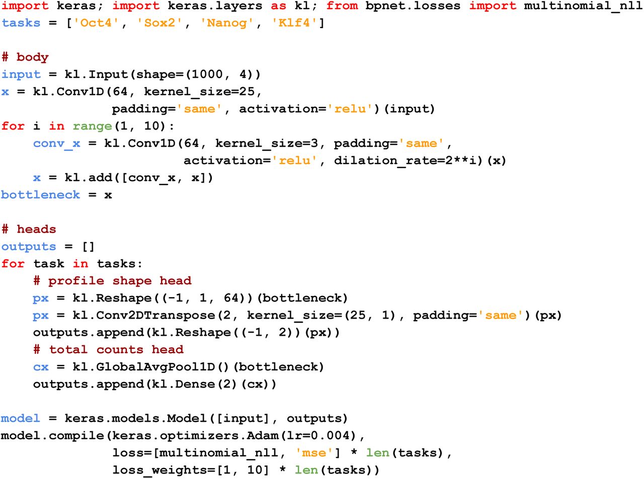
Loss function
Let kobs be the vector of length L of observed read counts for a particular strand and a particular task (i.e., transcription factor) along the sequence of length L. Let p pred be the vector of length L of predicted probabilities along the sequence, such that  and let
  be the total number of observed counts and npred the total number of predicted counts for the sequence. BPNet is trained using the following loss function for one particular sequence, strand and task:
 The first term evaluates the error in the shape of the predicted profile. It is the multinomial negative log-likelihood of observed base-pair read counts given the predicted probabilities and the total number of observed counts. The second term evaluates the squared error of the log total number of reads in the region. The total loss function is the sum of individual loss functions across both strands, all input sequences and all tasks (e.g. TFs).
The key question is how to choose a good value for the hyper-parameter λ. In supplementary text, we show that if  , where
  is the average number of total counts in our training set, the profile loss and the total count loss will be roughly given equal weight. As we will see later, we will use
  with α < 1 to upweight the profile predictions relative to the total count predictions.
Controlling for biases
Experimental assays such as ChIP-seq (and to a small extent also ChIP-nexus) have certain biases. These biases can be experimentally measured by performing control experiments such as input-DNA for ChIP-seq and PAtCh-CAP for ChIP-nexus (122). To prevent the sequence-to-profile model from learning these non-informative bias signals, the model tries to explain the target experimental track using both the sequence-based model predictions and the control experiment track
 Where fctl (ctl; wctl) is some transformation of the control track with the requirement that fctl (ctl; wctl) = 0 if the control track is 0 (i.e. bias not present). For the total count prediction head, fctl (ctl; wctl) is simply wctl log(1 + nctl), where nctl is the total number of reads from the control experiment in the modeled local region. For the profile prediction head, fctl (ctl; wctl) is a weighted sum of i) the raw counts and ii) a smoothed version of the raw counts using a sliding window sum of 50 bp. We use the sliding window to deal with typically very sparse data from the control experiment. During model training, the parameters of fctl (ctl; wctl) are also trained to best explain the output using the control track. We note that this framework also easily integrates multiple control tracks as well as control tracks predicted from sequence using a bias model learned on other data such as deproteinized genomic DNA for DNase-seq (131).
Training and hyper-parameter tuning
We used ChIP-nexus profiles of Oct4, Sox2, Nanog and Klf4 TFs in mouse embryonic stem cells (ESCs) to train and evaluate BPNet (100 million reads per TF, pooled from multiple replicates). The ChIP-nexus datasets exhibited high replicate concordance, signal-to-noise ratios and strong overlap of peaks with corresponding ChIP-seq experiments targeting the same TFs. PAtCh-CAP experimental data were used as the control. For each TF, the ChIP-nexus profile coverage is defined by the number of reads with the 5’ end aligned to a specific position and strand. Regions of enrichment (peaks) were identified using MACS2 (36) on smoothed read densities to obtain a ChIP-seq-like signal. We restrict model training and evaluation to 1 kb regions around the 147,974 summits in autosomes that ranked consistently across replicates genomic regions as measured by the irreproducible discovery rate (IDR) (130) threshold of 0.05. Regions from chromosomes 2,3,4 (20%) were used as the tuning set for hyper-parameter tuning. Hyper-parameters were manually adjusted to yield best performance on the tuning set. Regions from chromosomes 1,8,9 (20%) were used as the test set for final model evaluation. The remaining regions were used for model training.
We implemented and trained all neural network models in Keras (v2.2.4) (132) (TensorFlow backend v1.6) using the Adam optimizer (133) (learning rate = 0.004) and early stopping with patience of 5 epochs.
Profile evaluation metric
ChIP-nexus profiles contain TF footprints characterized by local spikes with high read counts surrounding a valley (putative TF binding site) with low read counts. Typical measures of similarity such as Pearson or Spearman correlation are not well suited to these types of profiles. To quantify the ability of the model to accurately localize footprint positions, we use a binary classification formulation to evaluate how well the model can distinguish positions with high read counts from lower read counts within each ChIP-nexus profile in the test set regions. Positions with more than 1.5% of the total number of reads in each 1kb test set region were labeled as belonging to the positive class and positions with less than 0.5% of total read counts were labeled as belonging to the negative class. These two thresholds were manually determined by visually inspecting the ChIP-nexus profiles in peak regions from the training chromosomes. The number of negative examples far outnumber the number of positive examples. Hence, we used the area under the Precision-Recall curve (auPRC) to evaluate the performance of the predicted read probability profiles relative to these binary labels. To evaluate the predictive performance at lower resolutions, we applied auPRC on binary labels and the predicted profile probabilities summarized in 2-10 bp long contiguous bins as follows: a bin was labeled as positive if there was at least one position in the bin with a positive label. If all the labels in the bin were negative, the bin was labeled as negative. Otherwise, the bin was labeled as ambiguous. For the predicted profile probabilities, the maximum value in the bin was used.
We used profiles sampled from replicate experiments to compute a corresponding upper bound for the above mentioned profile evaluation for each TF. For each TF, replicate experiments were divided into two groups with approximately equal numbers of sequencing reads. Read counts from one group were used as ground truth and the read counts from the other group were treated as a predictor similar to BPNet. The roles of the replicate groups were then swapped and the final predictive performance was averaged across both scenarios. Random baseline was obtained by using shuffled regions for model predictions.
DeepLIFT contribution score for sequence-to-profile models
DeepLIFT is a feature attribution method for computing the contribution of each base (feature) in an input sequence to a specific scalar output prediction from a neural network model (60). DeepLIFT decomposes the difference between the output prediction based on an input sequence and the output prediction based on a neutral reference input sequence (see below for definition of reference) as an additive combination of contribution scores of all bases (D features) in the input sequence:
 where ci is the contribution of feature i in input x to the model output prediction f (x) compared to model prediction f (r) based on the reference input r. We note that f () is a function returning a scalar. DeepLIFT was originally developed to compute the contribution scores with respect to a single scalar output e.g. predicted output read counts at a single position on a specific strand in a profile.
For BPNet, the profile output head for a particular TF returns a L × S tensor, where L is the sequence length and S is the number of output channels or strands for ChIP-nexus. Since the output of BPNet is a tensor and not a scalar, we needed to adapt DeepLIFT compute contribution scores with respect to the entire profile.
To compute base resolution contribute scores with respect to the entire output profile, we define the profile contribution score of a base as follows:
 Where pis is the predicted probability values for position i and strand s, obtained by normalizing the profile predictions on the logit scale using the softmax function along the sequence axis: p = softmax(f (x)). cis is the contribution score of the base with respect to the (scalar) profile prediction on the logit scale at position i and strand s. The rationale for performing a weighted sum is that positions with high predicted profile output values should be given more weight than positions with low predicted profile output values. The downside of such weighted sum formulation is that it would normally require the contribution scores to be computed L × S (=2,000) times for each 1 kb input sequence per TF.
To drastically speed up this computation we exploit the backpropagation algorithm used in DeepLIFT and the additive decomposition of DeepLIFT scores. We define a new TensorFlow operation as follows:
 where Const denotes the tf.stop_gradients operation which treats the wrapped expression pi (x) as a constant. By applying DeepLIFT to f^(x) we obtain, in a single DeepLIFT backpropagation step, the desired result:
 Therefore, the computational cost of computing the profile contribution scores is drastically reduced. Pseudo-code of the described op in TensorFlow code looks as follows:
We used all zeroes for the reference input since it showed the highest correlation with in-silico mutagenesis contribution scores. We used the DeepExplain implementation of DeepLIFT (repository fork available at https://github.com/kundajelab/DeepExplain/, commit hash: 738c7145e915a7a48f3a4248d088bcc2e1a94614) together with TensorFlow v1.6 to compute DeepLIFT contribution scores.
Motif discovery using TF-MoDISco
We computed the DeepLIFT profile contribution scores for each TF in all 1 kb peak regions from the training, validation and test set chromosomes (i.e. peaks from all autosomes). A null distribution of contribution scores was generated by randomly selecting 4,800 peaks, extracting the sequences, shuffling them and computing the profile contribution scores for the shuffled sequences. We shuffled the sequences in such a way that dinucleotide counts are preserved. TF-MoDISco (v0.5.1.1) was then run for each TF separately using the corresponding contribution scores of the TF in all regions where the corresponding TF was bound.
The TF-MoDISco algorithm (48) consists of three stages. In the first stage, the total contribution in sliding windows of length 21 (sliding_window_size) is computed, both for contribution scores from the real sequences and for contribution scores on the shuffled sequences. The distribution of sliding window scores on the shuffled sequences is used to define a ‘null distribution’ against which sliding windows from the real sequences that pass a FDR threshold of 0.01 (target_seqlet_fdr) are identified. Sliding windows are expanded on either side by 10 bp (flank_size) are selected in such a way that no two sliding windows overlap by more than 50%. The segments underlying these expanded sliding windows are termed ‘seqlets’, and are provided to the next stage for clustering. A total of 145,748 non-overlapping seqlets were identified. We limited the total number of seqlets to 50,000 for each run of TF-MoDISco in order to always satisfy the memory constraints (250GB).
In the second stage, seqlets are clustered into motifs. First, a similarity for each pair of seqlets is computed using the seqlet contribution scores. For a given pair of seqlets, different possible alignments of the seqlets are considered, and for every alignment, the similarity of the contribution scores is calculated using a correlation-like metric called continuous Jaccard (48). The best similarity across all alignments is then taken to be the similarity of the seqlet pair. The similarities of the seqlets are provided to a clustering algorithm, after transforming the similarities in a way that grants robustness to the fact that different clusters can have different densities. The clusters are found using a Louvain community detection algorithm (134) that automatically determines the number of clusters by optimizing graph modularity.
After the clusters have been identified, seqlets within a cluster are aligned to each other, and the coordinates of the seqlets are expanded to fill out any overhangs in the alignment. This kind of seqlet expansion makes it possible to discover motifs that are longer than the sliding window used for seqlet identification in the first stage. A Position Frequency Matrix (PFM) and a Contribution Weight Matrix (CWM) are computed from the aligned seqlets by averaging the base frequencies and the contribution scores respectively. The seqlet coordinates are then re-centered such that the region of highest contribution falls towards the middle of the CWM. Because these seqlet coordinates can be slightly different from the original seqlet coordinates, the second stage is run a second time using the seqlets with the new coordinates, for added robustness.
In the third and final stage, heuristics are applied to postprocess the motifs using the default TF-MoDISco settings for version 0.5.1.1. Clusters appearing to consist of two distinct motifs are split apart, following which clusters with highly similar motifs are iteratively merged. After all merging is complete, any clusters with fewer than 60 seqlets are treated as noise and disbanded, with their seqlets reassigned to larger clusters. Finally, motifs are expanded to the length of 70 bp and then trimmed down to their final lengths by removing flanking positions with an information content (IC) of less than 8% of the information of the base with the maximal information content in the motif. Motifs supported by less than 100 seqlets or with an information content smaller than 4 bits were discarded. The PFM information content is defined as:
 Where pi,j is the PFM value at position i and base j and bj is the background base probability (135). We used the following background base probabilities: A=0.27, C=0.23, G=0.23, T=0.27.
Identification of representative motifs
To identify and pairwise align similar motifs detected across different TFs, we performed the following motif clustering approach. First, we obtained all possible pairwise alignments of two motifs (i.e. all possible offsets and strand combinations) and identified the smallest continuous Jaccard distance metric (48) on the PFM information content. We then generated a pairwise distance matrix and performed hierarchical clustering in scipy (v1.2.1) using the Ward variance minimization algorithm (136) (method=’ward’) and optimal leaf ordering (137). Since many of these motifs were similar or discovered multiple times by different TFs, we clustered the motifs (Figure S3B) and manually selected 11 representative TF motifs of interest.
CWM scanning
To allow new sequences to be scored for motif instances similar to PWM scanning, we developed a method for scanning the contribution scores with the contribution weight matrix (CWM) from the TF-MoDISco motifs. We note that even though TF-MoDISco already identifies motif instances as seqlets, the detection of motif instances is not comprehensive since the number of considered seqlets (and hence the number of detected motif instances) was capped at 50,000 due to memory constraints.
There are three key differences between PWM and CWM scanning. First, a CWM instead of the PWM is used. CWM is obtained by averaging the contribution scores of all seqlets corresponding to a specific TF-MoDISco motif. Second, in CWM scanning, the contribution scores are scanned instead of the raw sequence. Third, we use a different similarity metric between the contribution scores and the CWM. Let wCWM ∈ ℝLW ×4 denote the CWM of length LW and C ∈ ℝLS ×4 denote the contribution scores for one-hot-encoded sequence s of length LS ≥ LW. The contribution score Ci,b for base b at position i is 0 if base b was not observed in the actual sequence (i.e. if si ,b = 0). We decompose the similarity metric between the CWM scanning position i of the contribution scores into two parts: i) the L1 norm of the contribution scores at positions between i and i + LW :
 and ii) the continuous Jaccard similarity measure between the CWM and L1 normalized contribution scores:
 where Jaccard(,) is the continuous Jaccard distance metric defined in (48). At each position i, the ‘match’ score (Scorematch) is computed for wCWM and its reverse-complement version. The maximum of the two scores is used as the final ‘match’ score at each position. Note that we did not scan the ‘hypothetical contribution’ scores as performed by TF-MoDISco since we observed a higher number of false positives using that approach.
To put the obtained scores into the perspective of original seqlets discovered by TF-MoDISco, we computed the ‘contrib’ and ‘match’ scores for all the seqlets at their extracted locations. That way, we obtain a distribution of scores determining the corresponding TF-MoDISco motif. We define the normalized ‘contrib’ score as the fraction of TF-MoDISco seqlets with a ‘contrib’ score smaller than the ‘contrib’ score of the CWM at a particular position.
A motif instance is called if:
- 20% or more of the TF-MoDISco seqlets had a ‘match’ score lower than the considered ‘match’ score
- At least one TF-MoDISco seqlet had a ‘contrib’ score lower than the considered ‘contrib’ score
- The classical PWM score is larger than 0.
We note that the CWM scanning procedure is purely sequence-based (like PWM scanning) and hence does not use the ChIP-nexus profile information.
We called motif instances in the union of 1kb wide TF peak regions (147, 974) on which TF-MoDISco was run. We scanned the contribution score of the corresponding TF from which the motif originated (e.g. we scanned Oct4 contribution scores for the motifs discovered by running TF-MoDISco on the Oct4 contribution tracks). We used the trimmed CWMs for scanning. We removed the motif instances of short motifs which overlapped any of the motif instances matching the long motifs (PFM information content IC>30).
Transposable element analysis
RepeatMasker annotations for mm10 obtained from http://www.repeatmasker.org/genomes/mm10/RepeatMasker-rm405-db20140131/mm10.fa.out.gz were used to compute the overlap of seqlets with transposable elements (TEs). A seqlet was considered to overlap a TE if it was fully contained within at least one element defined in RepeatMasker annotation. Kimura 2-parameters distance (138) between the seqlet sequence and the consensus sequence of the motif was used to sort the seqlets in Figure 4. This distance metric was re-implemented in Python and is equivalent to dist.dna function from R’s APE package with the model=’K80’ parameter (https://www.rdocumentation.org/packages/ape/versions/5.2/topics/dist.dna).
Motif pair strict spacing analysis
We obtained and filtered the 11 representative motif instances as described in previous section using CWM scanning. We discarded Sox2 sites overlapping the Oct4-Sox2 motif and removed palindromic motif pair matches. Motif pairs were considered when spaced center-to-center between 6 bp and 100 bp. Each motif pair was checked for overlap with RepeatMasker-annotated ERVK, ERVL, ERVL-MaLR, or ERV1 genomic regions. For each motif pair, histograms were generated comparing the spacing between each motif pair instance and its ERV overlapping class. The frequency of motif spacing relative to both the motif pair and the ERV overlapping class was computed for motif pairs that occurred more than 500 times across the genome.
TF-MoDISco motif validation
TF-MoDISco returned three short motifs not matching the canonical Oct4, Sox2, Nanog, or Klf4 binding motifs. Two of these motifs matched TF binding motifs for Zic3 and Esrrb as reported in literature. To confirm their motif identity, we performed Zic3 and Esrrb ChIP-nexus experiments and plotted their binding across the TF-MoDISco Zic3-like and Esrrb-like motifs. In both cases, this confirmed their identity.
TF-MoDISco returned three Nanog motifs with sharp and specific Nanog binding profiles. Nanog showed differences in binding across these three Nanog motifs. In order to test whether a binding partner was involved, we analyzed the Sox2 and Pbx binding profiles across these three Nanog motifs. No binding partner was identified.
Additionally, the reported binding motif of Pbx is similar to the identified Nanog motifs. To ensure that the Nanog motif was unique to Nanog, we analyzed Sox2, Pbx, and Nanog binding across the TF-MoDISco Nanog and Sox2 motif instances and the 5,000 top-scoring genomic matches with no mismatches to the Pbx motif TGAKTGACAGG.
One of the three short motifs did not appear to be a known TF motif important in ESCs. We queried the TRANSFAC database (139) using a motif identifier tool called TOMTOM from the MEME Suite (31). This revealed a match with sequences associated with TFIIIC subunits. Upon further inspection, this motif was revealed to be the TFIIIC B-box, a binding site that contributes to the recruitment of TFIIIC binding (140).
TFIIIC B-Box and tRNAs
The TF-MoDISco-returned B-box was the only motif identified associated with Pol III. Consistent with this motif being a Pol III motif, we found that the TFIIIC B-box motif frequently overlapped with tRNA genes across the mouse genome. The tRNA genes were obtained from the tRNAscan-SE predictions stored in GtRNAdb 2.0 (141). We then classified the B-box motifs based on their gene overlap and computed the average phastCon score (phastCons60way.UCSC.mm10) over each motif instance as a measure of vertebrate conservation (142). We also computed the copy number of the tRNAs overlapping with the B-box motifs based on amino acid anti-codons, separating methionine (Met) and activated methionine (iMet) as two separate amino acid classes.
Pairwise motif interaction analysis
We studied the pairwise interaction between the following motifs discovered by TF-MoDISco:
- Oct4-Sox2 (pattern 0 from Oct4, consensus=TTTGCATAACAA),
- Sox2 (pattern 1 from Sox2, consensus=GAACAATGG),
- Nanog (pattern 1 from Nanog, consensus=AGCCATCA),
- Klf4 (pattern 0 from Klf4, consensus=CCACGCCC).
We considered motif instance pairs (A, B) spaced at some distance d<160 bp and compared BPNet ChIP-nexus profile predictions between 4 cases: where either motif A or B was replaced by a random sequence, where both were replaced by a random sequence or where both were left intact. Motif instance pairs were either simulated in synthetic sequences or were detected by CWM scanning in sequences underlying ChIP-nexus peaks (Figure S5A).
Synthetic sequences
For synthetic sequences, we first created 128 random sequences of 1 kb in length by sampling the base at each position with equal probability. Next, we replaced the central bases by the consensus sequence of motif A and similarly inserted motif B d bases downstream of A (d is the distance between motif centers). We used BPNet to predict the stranded ChIP-nexus profile for the primary TF of motif A (e.g. Oct4 for the Oct4-Sox2 motif and Nanog for the Nanog motif). We averaged the predictions across the 128 random sequences to obtain the marginal predicted profile PAB. We repeated the same procedure by i) inserting only the motif A in the center (PA), ii) inserting only the motif B d-bases downstream of the center, and iii) not inserting any motif and hence only averaging the predictions across random sequences (PØ). We used the predicted profile PA to determine the predicted summit location within 35 bp of the motif A center for each strand. The stranded summit location at motif A was then used to determine the profile height in all 4 scenarios averaged across the two strands. We denote average predicted profile height of the 4 different predicted profiles (PA, PB, PAB and PØ) by hA, hB, hAB, and hØ correspondingly. We define the corrected binding fold change quantifying the influence of motif B on motif A as:
 The binding fold change of 1 denotes that profile height of A is the same whether or not motif B is present in the vicinity of A. If the fold-change is higher than one, then the profile of A is higher compared to the case where B is absent. We note that the second term in the numerator (hB – hØ) corrects for the tail of the motif B profile which occurs when motif A and B are close to each other.
We performed the analysis for all motif pairs, strand orientations and possible pairwise distances ranging from 11 bp to 160 bp.
Genomic sequences
To compute the corrected binding fold-change of motif interactions in genomic sequences, we first obtained motifs instance locations in 1 kb ChIP-nexus peak regions using CWM scanning. We discarded motif instances from duplicated peak regions overlapping other peak regions by more than 200 bp as well as motif instances overlapping TEs (discovered by TF-MoDISco and mapped back to the genome using CWM scanning). Also, Sox2 motif instances overlapping the Oct4-Sox2 motif were discarded. For each motif pair, 4 model predictions were made:
- PAB: the reference sequence of the whole interval in which the motifs were present
- PA: motif instance B replaced by random sequence
- PB: motif instance A replaced by random sequence
- PØ: motif instances A and B replaced with random sequence
We computed the profile heights at motif A profile summit locations in the same manner as for the synthetic sequences yielding 4 profile heights: hA, hB, hAB, and hØ. We added “pseudo counts” defined as the 20th percentile of the considered quantity to the tail-corrected profile height of the reference sequence: hAB – (hB – hØ) + PCAB as well as the profile height of the A-only sequence: hA + PCA. Next, we kept only the motif pairs where the tail-corrected profile height of the motif was in the top 20% for both motifs. This ensured that only motif pairs showing a footprint were used. Finally the corrected binding fold-change was computed for each motif instance pair as:
 We note that there are three main differences between the synthetic and genomic sequences. First, in genomic sequences, the background sequences were not random and may contain other motifs. Second, the “perfect” consensus sequence was used for injecting motifs in synthetic sequences, whereas for genomic sequences the motif sequence rarely matched the consensus. Third, the distribution of motif pairwise distances in genomic sequences is not perfectly uniform as for the synthetic case, hence some pairwise distances might be under-represented.
Motif pair likelihood of occurrence analysis
We obtained and filtered motif instances as described in previous section using CWM scanning. We discarded Sox2 sites overlapping the Oct4-Sox2 motif. To compute whether motif A is located close to B more frequently than expected by chance, we counted i) the number of times a motif instance A is close to motif instance B and ii) the number of times motif instance A is close to motif instance B if we shuffle all motif instances between peaks while maintaining the relative location within the peak. We constructed the following 2-by-2 contingency matrix cm :
 and applied the Pearson’s Chi-square test (chi2_contingency from scipy.stats) to observe the p-value quantifying whether the odds-ratios (A close vs not close to B) between the observed and shuffled motif instances are significantly different. Finally, we use the odds-ratio to visualize whether A is closer to B more frequently than expected by chance:

Benchmarking alternative methods: ChExMix
ChExMix v0.3 with default parameters was run for each TF on the pooled BAM file containing reads of all the replicates for the corresponding TF. The same blacklisted regions (--exclude) as for peak calling in the ChIP-nexus pipeline were used. The following mm10 background file (--back) was used (http://lugh.bmb.psu.edu/software/chexmix/backgrounds/mouse.back).
Protein structure visualizations
The structure of Sox2 and Oct1 bound to DNA in Figure 3A was rendered in VMD (143) using secondary structure information from STRIDE (144) and surfaces from SURF (145), based on the NMR structure 1O4X (146). This Sox2-Oct1-DNA model has been used as a homology model to build the Oct4-Sox2-DNA complex (146), and is therefore representative of the structure of that complex, but coordinates for that model have not been made available.
The nucleosome structure in Figure 5 was rendered in Povray 3.7 (147) from a structure generated by VMD based on the crystal structure 1AOI (148).
Periodicity comparisons
SASA values were calculated in VMD (143) with a 4 Å probe radius. Each nucleobase was considered independently, and the SASA values from each base pair (one from each strand) were added together to give the total SASA values (Figure S8).
Dinucleotide AA/AT/TA/TT frequencies were calculated across nucleosomes mapped by (149) using deconvolved chemical mapping cleavage information (GEO accession GSE82127).
Frequencies were then averaged to provide a consensus AA/AT/TA/TT frequency profile across murine nucleosomes.
Software availability
Code to reproduce the results of this manuscript is available at https://github.com/kundajelab/bpnet-manuscript. We also streamlined and generalized this code into a bpnet python package (https://github.com/kundajelab/bpnet/) with functionality to train and interpret base-resolution deep neural networks trained on the coverage tracks of any functional genomics assay. The ChIP-nexus data processing pipeline which includes read trimming, mapping, peak calling and generating the coverage tracks is available at https://github.com/kundajelab/chip-nexus-pipeline. The nimnexus software package for trimming and de-duplicating ChIP-nexus sequencing reads is available at https://github.com/Avsecz/nimnexus/.
Supplementary text 1: Method comparison
ChExMix and PWM scanning

A) Motifs discovered by ChExMix run on Oct4, Sox2, Nanog and Klf4 ChIP-nexus data. B) ChIP-nexus profile height distribution at BPNet motif instances for different TFs. The vertical grey lines denote the 90th percentile which is used as a stringent threshold for determining motif instances showing a ChIP-nexus footprint. C) Number of motif instances showing a footprint (y-axis) as measured by the ChIP-nexus profile height larger than the threshold defined in B within the top N motif instances prioritized by the corresponding method (x-axis). Only motif instances overlapping the peak regions as called by MACS2 from the held-out test chromosomes (1, 8 and 9) were used. A high motif contribution score was used to prioritize motif instances for BPNet, a high PWM score for PWM, and high profile score for ChExMix. Note that BPNet and PWM methods do not use the profile information whereas ChExMix is already using the read distribution at the motif instance to determine the profile score. D) PFM and the aggregate ChIP-nexus footprint (Obs in orange) for all Nanog-Nanog pairs with the same orientation spaced at 10bp (left) or 40bp (right) as discovered by BPNet. The average BPNet prediction (red) and the mixture of two individual average Nanog footprints (blue) were scaled to have the same number of total counts as the observed profile.
To evaluate the extent and quality of motifs discovered by BPNet in the light of previous methods, we compared our approach to ChExMix (28). ChExMix is a state-of-the-art motif discovery and TF binding event calling method for ChIP-exo and ChIP-nexus data. We ran ChExMix on each of the studied ChIP-nexus data for each TF (Oct4, Sox2, Nanog and Klf4) and observed 5 motifs in total (Figure 1A). These were the cognate motifs for each of the TFs: Oct4-Sox2, Sox2, Nanog and Klf4. Motifs with fuzzy indirect footprints such as Zic3, B-Box, Essrb, or dimer-motifs such as Oct4-Oct4 or other motif variants were not discovered. We speculate that these motifs were missed because of lower number of reads and heterogeneous profile shapes (especially for the fuzzy footprints). Moreover, ChExMix also did not discover long TE motifs. Although changing the parameters in the motif discovery step of ChExMix may allow the discovery of some TEs, the dependence on these parameters makes it difficult for ChExMix to discover TEs alongside short motifs in a flexible manner. We conclude that the motifs discovered by BPNet extend well beyond the motifs discovered by ChExMix.
To evaluate the quality of the called motif instances in the genome, we compared the BPNet approach using CWM scanning to classical position weight matrix (PWM) scanning. Unlike ChExMix (see below), both CWM scanning (BPNet) and PWM scanning only use the sequence information to identify motif instances and can thus be directly compared. To score the quality of the identified motif instances, we determined their ChIP-nexus profile heights, as measured by the number of ChIP-nexus reads at the maximum position in the motif vicinity (+-35bp from the motif center). The results show that the contribution scores of (BPNet) CWM motif instances correlated much more strongly with maximum profile heights than the PWM affinity score of instances identified by PWM scanning (Main Figure 2F). This implies that the contribution scores are a better proxy for TF occupancy than the PWM score. This makes sense since contribution scores consider the entire sequence context of the motif within the 1 kb region and thus can integrate more information relevant for TF binding. By contrast, the PWM is limited to the local sequence context (<20 bp) and does not consider the possible interactions between nucleotides and motifs.
Since the contribution scores correlated much better with the ChIP-nexus profile height than the PWM score, we asked whether this approach also improved the often criticized high false positive rate of motif instances obtained by PWM scanning. To determine the false positive rate of the motif instances in the test chromosome, we considered sites with the ChIP-nexus profile height above the 90th percentile as true binding sites (Figure B). Since the number of binding sites depends on the used cutoff, we treated the evaluation as a ranking or prioritization problem. Indeed, motif instances derived by CWM scanning prioritized more binding sites with high ChIP-nexus counts and thereby exhibited a lower false positive rate compared to PWM scanning (Figure 1C). This difference is especially profound for the short Nanog motif. Even though the CWM has the same length as the PWM, the contribution scores scanned by the CWM already consider the context of the motif. Hence, the Nanog motif can get a higher contribution score if it is present in the vicinity of other ∼10bp spaced Nanog motifs. Hence, our approach of scanning the contribution scores using the CWM (instead of the raw sequence using the PWM) greatly reduces the false positive sites while still following the familiar scanning procedure as with PWMs.
We also compared the motif instance scoring to ChExMix. ChExMix directly uses the profile information from the ChIP-nexus data to determine motif instances. As expected, ChExMix recalls more binding sites with high ChIP-nexus counts. However, we note that this comparison is circular since the profile information used to evaluate the motif instances is also used to call them. By contrast, the CWM scanning of BPNet relies only on the DNA sequence and its corresponding base resolution contribution scores (also computed from the DNA sequence). We performed the evaluation on the test chromosomes held-out from BPNet training which guarantees that BPNet has never seen the ChIP-nexus data used in this evaluation. Interestingly, we observe that ChExMix plateaued at about 500 to 1200 called motif instances with high profile scores, whereas the CWM scanning was able to recall more binding sites in total. The lower number of binding events discovered by ChExMix could be caused by the limited number of mapped reads at base-resolution (despite the overall high sequencing depth of >100M) which limits the ability to reliably detect footprints from the read coverage profiles.
Next, we asked whether the higher false positive rate of PWM scanning or the limited number of motif instances discovered by ChExMix impair the discovery of 10bp Nanog-Nanog spacing in the genome as discovered by BPNet. Indeed, we found that the Nanog-Nanog pairwise spacing histograms showed only weak signs of 10 bp periodicity for both methods (main Figure 6B,C). For PWM scanning, the high false discovery rate of motif instances likely prevents the detection of Nanog’s 10 bp periodicity. For ChExMix, we observed a depletion of instances below 40 bp where most of the spatially constrained Nanog instances were discovered by CWM scanning (main Figure 6A). This depletion of motif instances at close proximity could be due to two reasons. First, the optimized likelihood of ChExMix is non-convex and hence the global optimum might be difficult to find and may strongly depend on the initial conditions. Second, the key assumption of ChExMix is that the tag distribution (representing the average profile) associated with a specific motif is constant. However, this assumption is an oversimplification since ChIP-nexus profiles associated with a motif can change their form in the presence of motifs of other cooperatively bound TFs. For example, Figure 1D shows the difference between the observed average footprint of two nearby Nanog motifs (orange) and the mixture of the individual two motifs (blue). If the two Nanog motifs are frequently co-bound as a homo-dimer, the inner parts of the dimer will be less accessible by exonuclease resulting in a lower number of cut sites in the inner peaks compared to the outer peak sites. Hence, the ChIP-nexus profiles of co-bound TFs can be less accurately represented by the mixture of the two independent ChIP-nexus profiles distributions as modelled by ChExMix. Interestingly, BPNet (shown in red) does not simply model the data as an explicit mixture and correctly captures the depletion of ChIP-nexus counts in the center.
Profile regression as performed by BPNet yields more motifs and better motif instances compared to binary peak classification
A frequently used approach for training deep learning models is to treat the TF binding prediction as a binary classification problem (41, 42). In this approach, the training examples are sequences extracted from contiguous bins in the genome and the sequence label is positive if a TF binding peak overlaps the bin region (and negative otherwise). The benefit of such an approach is two fold. First, the assay-specific biases are already accounted for in the peak-calling process. Second, the resulting machine learning task – binary classification – is well understood. Hence the standard loss function such as binary cross-entropy and the standard evaluation metrics such as the area under precision-recall curve (auPRC) can be used. However, compressing the observed data into binary labels discards information about the strength of binding present in the total number of reads and specific details of the binding or co-binding mode present in the read coverage profile shape.

A) Predictive performance of the binary classification models predicting the presence or absence of ChIP-nexus peaks from 1 kb DNA sequences evaluated across the held-out (tuning) chromosomes 2, 3, and 4. The model trained to classify the sequences is shown in orange and the model trained to also predict the ChIP-nexus profiles from DNA sequence in addition to classifying them is shown in green. B) Training time of the binary classification model trained genome-wide and the sequence-to-profile model (BPNet) trained in ChIP-nexus peaks. C) Detected motifs by TF-MoDISco using the contribution scores in ChIP-nexus peaks of the sequence-to-profile BPNet (profile reg.) or the binary classification model (binary class). A light color denotes a high number of seqlets for each motif. Motifs not discovered or motifs supported by less than 100 seqlets are shown in black. Questionable motifs are displayed separately on the right. D) The number of motif instances showing a ChIP-nexus footprint (y-axis) within the top N motif instances with highest contribution scores (x-axis) from the held-out (test) chromosomes 1, 8 and 9. A site was considered to show a ChIP-nexus footprint if the number of reads at the position of the aggregate footprint summit (averaged across both strands) is higher than the 90th percentile value of all motif instances detected by the profile regression model for the corresponding TF (same as in Figure 1C).
To investigate the benefit of training the model on the ChIP-nexus read coverage tracks as performed by BPNet to the frequently used binary classification, we modified the BPNet architecture and replaced the output heads performing profile regression with the output heads performing binary classification. These consisted of weighted global average pooling using spline transformation (150) and a dense layer followed by sigmoid activation. We trained the model on contiguous bins of 50 bp (flanked to 1 kb) spaced across the genome and labeled them as positive if the central 200bp of the bin overlapped the peak as called by MACS2. The predictive performance on the held-out tuning chromosomes (2, 3 and 4) was 25% auPRC in average across the 4 TFs after tuning the optimal learning rate (Figure 2A). We also observed that training the binary classification model genome-wide took 3 times longer to train (Figure 2B) than BPNet, which is trained only on 147,974 peak regions. To ensure that the dilated convolutional layers are also appropriate for binary classification, we trained and evaluated the Basset (46) and factorized Basset (151) architectures. After tuning the dropout rate with random search, we obtained a slightly lower auPRC of 24% for both models, suggesting that our original architecture with dilated convolutions was also a good fit for binary classification. Next, we asked whether the predictive performance of the binary classification model could be improved by adding another output head predicting the stranded ChIP-nexus profile as originally done by BPNet. Indeed, the classification performance increased for all TFs yielding an average of 31% auPRC (Figure 2A). We conclude that the read coverage track indeed provides additional information not captured by the binary labels and allows learning more informative features in the shared convolutional layers.
We next asked whether the contribution scores of the profile regression model highlight additional motifs compared to the binary classification model. We computed the DeepLIFT contribution scores for each TF (pre-sigmoid activation) and ran TF-MoDISco in the same regions with the same hyper-parameters as previously done for BPNet. We clustered the discovered motifs based on their PFM similariy and manually assigned motif labels as done in Supplementary Figure S3B. TF-MoDISco using the contribution scores of the binary classification model discovered 9 out of 11 main short motifs found by the profile regression model BPNet (Figure 2C, Supplementary Table 2). The 2 missed motifs, Oct4 monomer and B-Box, are hence not frequently used by the model to predict the presence or absence of the peak as they might co-occur with other more predictive motifs. Interestingly, a higher number of questionable motifs including GC sequence composition bias motifs, ambiguous motifs and degenerate or noisy motifs was discovered from the contribution scores of the binary classification model. This suggests that the contribution scores of the binary classification model might be noisier than for the profile regression model. Nevertheless, we note that high reproducibility of the discovered motifs using two different models trained on similar but different data demonstrate the robustness of TF-MoDISco.
To compare the accuracy of motif instances called in the genome for the 4 cognate motifs discovered by TF-MoDISco for both models (Oct4-Sox2, Sox2, Nanog and Klf4), we performed the instance ranking analysis as for ChExMix considering sites with high ChIP-nexus profile as valid binding sites. The contribution scores of both models yielded a similar recall of Oct4-Sox2 and Sox2 motifs with high ChIP-nexus profiles (Figure 2D). We speculate that since the two motifs are linked to the pioneering activity, the binding sites will be important for binary classification and will hence not be missed by the binary classification model. Strikingly, the BPNet contribution scores of motif instances recalled a much higher fraction of Nanog motifs with high ChIP-nexus profiles (Figure 2D). Since Nanog is frequently co-bound either as a homo-dimer or as a hetero-dimer with Sox2, the ChIP-nexus profile shape contains rich information about this binding event. Since BPNet is trained on ChIP-nexus profiles directly, it is able to yield much more accurate contribution scores and thereby call motif instances with fewer false-positives. Altogether, we observe that learning to predict the full ChIP-nexus profiles as done by BPNet instead of just binary classes reduces the training time by three fold, increases the number of discovered motifs with strong seqlet support, and increases the quality of the called motif instances. Moreover, the profile predicted by BPNet assesses binding at individual motifs which offers a higher resolution to study the directionality of TF binding syntax as shown in the main Figure 5.
BPNet is also applicable to ChIP-seq

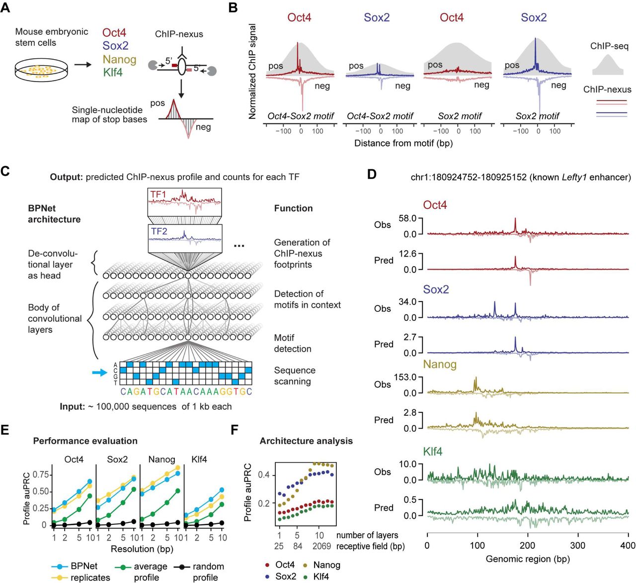
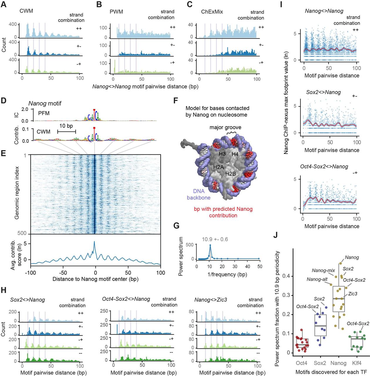
A) Observed and predicted read counts for BPNet trained on ChIP-seq data for the Zfp281 and Letfy1 enhancers located on the held-out (test) chromosome 1. Reads mapping to the forward strand are displayed in dark and reads mapping to the reverse strand in light. For the observed read counts, a sliding window of 50 bp was used to smooth the raw 5’ end read counts (line). Raw counts are shown as points on the bottom at y=0. B) BPNet predicts the ChIP-seq profile shape better than the replicates. Multinomial-log likelihood given the observed number of total counts was used to evaluate the profile shape quality at different resolutions (from 1 bp to 10 bp windows) in held-out chromosomes 1, 8 and 9 (Methods). A log-likelihood of 0 corresponds to the constant model. C) Total counts in the 1kb regions centered at the peak summits in the region can be predicted (blue) at a decent accuracy level as measured by Spearman correlation but doesn’t surpass replicate performance (green). D) Observed and predicted read counts as well as the contribution scores of BPNet for the known Oct4 enhancer. As for A, the observed read counts are shown both as smoothed (line) and as raw counts (points at y=0). Motif instances derived by CWM scanning are highlighted with a green box. E) BPNet applied to ChIP-seq discovers the majority of the motifs identified by BPNet applied to ChIP-nexus data. The models ‘ChIP-nexus profile cr’ and ‘ChIP-seq profile cr’ were trained on the union of the ChIP-nexus/seq peaks predicting Oct4, Sox2, and Nanog binding and were interpreted on the intersection of the ChIP-nexus/seq peaks. F) Motif instance calling with CWM scanning has higher accuracy for BPNet trained on ChIP-nexus data than for BPNet trained on ChIP-seq data. Additionally, training a sequence-to-profile model on ChIP-seq data yields a higher accuracy than training a binary classification model. See Figure 2E legend for detailed description.
The BPNet model together with the interpretation workflow using DeepLIFT and TF-MoDISco can be readily applied to ChIP-seq, since it does not make any modeling assumptions specific to ChIP-nexus profile shape. The major difference of ChIP-seq compared to ChIP-exo/nexus is that the 5’ ends of the reads mapping to a particular strand are dispersed in a 100-200 bp window around the peak whereas the ChIP-exo/nexus peaks frequently achieve base-resolution. To demonstrate that BPNet is also applicable to ChIP-seq, we performed ChIP-seq for 3 out of 4 previously studied TFs (Oct4, Sox2 and Nanog). We processed the data using the ENCODE ChIP-seq pipeline and generated the strand-specific 5’ read count tracks as for ChIP-nexus. We used the same architecture structure for ChIP-seq as for ChIP-nexus and determined the optimal hyper-parameters using a hyper-parameter search. We observed that the BPNet model for ChIP-seq overall required the same hyper-parameters as for ChIP-nexus. The only hyper-parameter that differed was the increased width (50) of the deconvolutional layer (compared to 25 which was optimal for ChIP-nexus). Similar to the ChIP-nexus control experiment PAtCh-Cap, we used the ChIP-seq input control experiment using an unspecific antibody in the loss function to control for the biases (Methods). We also added data augmentation (genomic intervals shifted uniformly from [-200, 200] bp with random reverse complementation). This is more important when ChIP-seq data are trained on peaks only since the shape of the profiles will be fairly constant hence a constant model can already fit the data well.
To gain intuition about the prediction quality of BPNet compared to replicate experiments, we investigated the known Zfp281 and Lefty1 enhancers as done before for ChIP-nexus data. Since the model evaluation was performed in peak regions, we added data augmentation (genomic intervals shifted uniformly from [-400, 400] bp with random reverse complementation) to make sure the model doesn’t simply predict the average ChIP-seq signal centered at the peak. We observed that the predicted profile shapes indeed resemble the smoothed ChIP-seq signal (averaging sliding window of 50bp, Figure 3A). To evaluate the predictive performance of the ChIP-seq BPNet model, we performed a similar analysis as for ChIP-nexus with the difference that we assessed the quality of profile shape prediction using the multinomial log-likelihood. We found that BPNet outperformed the smoothed replicate experiments in terms of profile shape prediction on almost all TFs except Nanog where both performed similarly (Figure 3B). The total count predictions of BPNet were not as good as replicate experiments (Figure 3C). As already discussed for BPNet trained on ChIP-nexus data, the total counts can be influenced by DNA accessibility which depends on a larger chromatin context. Altogether, we conclude that BPNet is applicable to ChIP-seq where it also shows high predictive accuracy on par with replicate experiments.
Next, we investigated the contribution scores of BPNet trained on ChIP-seq data in the known Oct4 enhancer. The contribution scores were computed in the exact same manner as for the ChIP-nexus model. We found that the contribution scores also precisely highlighted the Oct4-Sox2 motif in the center and the Nanog motif on the side (Figure 3D). Hence, we were able to directly apply the BPNet model to ChIP-seq data and have obtained accurate predictions as well as contribution scores highlighting the expected regulatory motifs.
To test which motifs were learned by BPNet applied to ChIP-seq, we used TF-MoDISco with the same hyper-parameters as before. To compare the results to models trained on ChIP-nexus data, we trained additional models on ChIP-nexus and ChIP-seq data in the same set of common regions (union of ChIP-nexus and ChIP-seq peaks), for the same TFs (Oct4, Sox2, Nanog), and used the same set of regions (intersection of ChIP-nexus and ChIP-seq peaks) for model interpretation.
Additionally, to compare the benefit of using a profile regression model for ChIP-seq, we trained a binary classification model on ChIP-seq data in the same manner as done before for ChIP-nexus data. We observed that TF-MoDISco applied to ChIP-seq discovered the majority of the expected motifs for all models (Figure 3E, Supplementary Table 2). A higher number of questionable motifs was obtained only for the binary classification model. These results show that BPNet trained on ChIP-seq data performs comparably well to BPNet trained on ChIP-nexus data in terms of motif discovery.
To determine the quality of the motif instances obtained by the four models, we performed the same motif instance prioritization analysis as before in Figure 1C and Figure 2D. We observed that BPNet trained on ChIP-nexus data (labelled “ChIP-nexus profile cr”) recalled a higher fraction of motif instances with high ChIP-nexus signal for the Nanog motif compared to BPNet trained on ChIP-seq data (labelled “ChIP-seq profile cr”). Both models performed similarly well for Oct4-Sox2 and Sox2 motifs. Additionally, BPNet trained on ChIP-seq data yielded better motif instances than a binary classification model trained on the same data (ChIP-seq profile vs ChIP-seq binary). Since the BPNet trained on ChIP-seq data outperforms a binary classification model and a model trained on ChIP-nexus data outperforms a model trained on ChIP-seq data, we conclude that the resolution of the modeled data is critical for accurate motif instance calling.
Altogether, these results show that our entire BPNet workflow, which includes BPNet training, motif discovery with TF-MoDISco, and determining motif instances with CWM scanning, can be readily applied to ChIP-seq data. These results were obtained with very minor hyper-parameter adjustments while explicitly controlling for assay specific biases. Hence, it should be possible to adapt and apply the BPNet workflow to other genome profiling assays exhibiting footprints such as ATAC-seq, DNase-seq or CUT&RUN.
Supplementary text 2: Relationship between the Poisson log-likelihood, mean-squared error and multinomial log likelihood
We start by writing down the negative log-likelihood for the Multinomial distribution. Let L be the sequence length, N the total number of events (i.e. total number of read counts in the region) and pi the probability of obtaining the outcome i (e.g. the read gets aligned to position i). Then, the negative log likelihood can be written as
 Note that we gathered all the terms independent of pi ∀i into the constant M. Let’s assume the read counts at each genomic location ki are distributed according to the Poisson distribution. The Poisson log likelihood for the sequence region of length L can be written as
 If we replace μi with Np pi, where Np is the predicted number of total counts and use
  , we obtain:
 We observe that the second term equals to the multinomial negative log-likelihood. If we set Np = elog Np, N = elog N, and perform a Taylor expansion
 up to the squared term for variable log Np around log N using, we obtain:
 This means that we can approximate the Poisson log-likelihood by a sum of mean-squared errors and the multinomial loss function where the predicted log of total counts log Np is close to the true total counts log N :
 We approximate the expression further by replacing the N in front of MSE with
  , where
  is the average (or median) value of N across the dataset and α is the tuning parameter which allows to up or down-weight the importance of total count prediction:
 If α =1, the multinomial loss and the mean squared error loss are balanced according to the Poisson log-likelihood.
Acknowledgements
We thank Mike Levine (Princeton) and Robb Krumlauf (Stowers Institute) for comments on the manuscript and Johnny Israeli for technical help at the beginning of the project. This work was funded by the Stowers Institute for Medical Research, the NIH grant 1R01HG010211 to J.Z., and the NIH grants 1DP2GM123485, 1U01HG009431 and 1R01HG009674 to A.K.. Ž.A. was supported by the German Bundesministerium für Bildung und Forschung (BMBF) through the project MechML (01IS18053F). A.S. was supported by the Stanford BioX Fellowship and the HHMI International Student Research Fellowship.
References
- 1.↵
- 2.
- 3.↵
- 4.↵
- 5.↵
- 6.
- 7.
- 8.
- 9.
- 10.
- 11.
- 12.↵
- 13.↵
- 14.↵
- 15.
- 16.↵
- 17.↵
- 18.↵
- 19.↵
- 20.↵
- 21.↵
- 22.
- 23.↵
- 24.↵
- 25.↵
- 26.↵
- 27.↵
- 28.↵
- 29.↵
- 30.↵
- 31.↵
- 32.
- 33.
- 34.↵
- 35.↵
- 36.↵
- 37.
- 38.
- 39.
- 40.↵
- 41.↵
- 42.↵
- 43.↵
- 44.↵
- 45.↵
- 46.↵
- 47.
- 48.↵
- 49.↵
- 50.↵
- 51.↵
- 52.↵
- 53.↵
- 54.↵
- 55.↵
- 56.↵
- 57.↵
- 58.↵
- 59.↵
- 60.↵
- 61.↵
- 62.↵
- 63.
- 64.
- 65.
- 66.↵
- 67.↵
- 68.↵
- 69.↵
- 70.↵
- 71.↵
- 72.↵
- 73.↵
- 74.↵
- 75.
- 76.
- 77.
- 78.↵
- 79.↵
- 80.↵
- 81.↵
- 82.↵
- 83.↵
- 84.↵
- 85.↵
- 86.↵
- 87.↵
- 88.↵
- 89.↵
- 90.↵
- 91.↵
- 92.
- 93.↵
- 94.↵
- 95.↵
- 96.↵
- 97.↵
- 98.↵
- 99.↵
- 100.
- 101.
- 102.↵
- 103.
- 104.↵
- 105.↵
- 106.↵
- 107.↵
- 108.↵
- 109.
- 110.
- 111.↵
- 112.↵
- 113.↵
- 114.
- 115.↵
- 116.↵
- 117.↵
- 118.↵
- 119.↵
- 120.↵
- 121.↵
- 122.↵
- 123.↵
- 124.↵
- 125.↵
- 126.↵
- 127.↵
- 128.↵
- 129.↵
- 130.↵
- 131.↵
- 132.↵
- 133.↵
- 134.↵
- 135.↵
- 136.↵
- 137.↵
- 138.↵
- 139.↵
- 140.↵
- 141.↵
- 142.↵
- 143.↵
- 144.↵
- 145.↵
- 146.↵
- 147.↵
- 148.↵
- 149.↵
- 150.↵
- 151.↵


