

Abstract
Evolutionary rescue is the process by which a declining population successfully adapts genetically to avoid extinction. In a subdivided population composed of different patches that one after the other deteriorate, dispersal can significantly alter the chances of evolutionary rescue of a wild type population not viable in deteriorated patches. Here, we investigate the effect of different dispersal schemes and intensities on the probability of successful establishment of a mutant population, adapted to the deteriorated environment. As a general pattern we find that the probability of evolutionary rescue can undergo up to three phases when varying the rate of dispersal: increasing the dispersal rate (i) at low dispersal rates the probability of establishment of a mutant population increases; (ii) for intermediate dispersal rates the establishment probability decreases; and (iii) at large dispersal rates the population homogenizes, either promoting or sup-pressing the process of evolutionary rescue, dependent on the fitness difference between the mutant and the wild-type. Our results show that habitat choice, when compared to uniform dispersal, impedes successful adaptation when the mutant has the same habitat preference as the wild type, but promotes adaptation when the mutant mainly immigrates into patches where it has a growth advantage over the wild type.
1 Introduction
Facing current anthropogenic environmental changes such as deforestation, soil and water contamination or rising temperatures, populations of many species are declining and might eventually go extinct(Bellard et al., 2012; Diniz-Filho et al., 2019). Pests and pathogens experience similarly strong selective pressures as a result of increased consumption of antibiotics and use of pesticides. This has led to the evolution of resistant genotypes (Ramsayer et al., 2013; Kreiner et al., 2018). The process of genetic adaptation that saves populations from extinction is termed evolutionary rescue. It is defined as an initial population decline followed by recovery due to the establishment of rescue types, (ideally) resulting in a U-shaped demographic trajectory over time (Gomulkiewicz and Holt, 1995). In recent years, empirical examples of evolutionary rescue have accumulated (Alexander et al., 2014; Carlson et al., 2014; Bell, 2017). It has been observed both in wild populations (e.g. Vander Wal et al., 2012; Di Giallonardo and Holmes, 2015; Gignoux-Wolfsohn et al., 2018) as well as laboratory experiments (e.g. Bell and Gonzalez, 2009; Agashe et al., 2011; Lachapelle and Bell, 2012; Lindsey et al., 2013; Stelkens et al., 2014).
In mathematical models, evolutionary rescue is often studied in a spatially homogeneous situation where the whole population experiences a sudden decrease in habitat quality. In this setting, a large number of theoretical results have been established; these concern, for example, the effects of recombination (Uecker and Hermisson, 2016) and horizontal gene transfer (Tazzyman and Bonhoeffer, 2014), reproduction mechanisms (Glémin and Ronfort, 2013; Uecker, 2017), intra- and interspecific competition (Osmond and de Mazancourt, 2013), predation pressure (Osmond et al., 2017), bottlenecks (Martin et al., 2013), and the context-dependent fitness effects of mutations (Anciaux et al., 2018). In fragmented environments however, habitat deterioration is not necessarily synchronized across patches, involving a transient spatially heterogeneous environment consisting of old- and new-habitat patches until eventually the whole environment has deteriorated. If individuals that populate different patches are able to move between those, the effect of dispersal on evolutionary rescue needs to be taken into account (Uecker et al., 2014; Tomasini and Peischl, 2019). Experiments that study the effect of dispersal on evolutionary rescue are rare but indicate that even low dispersal rates can significantly increase the likelihood of successful genetic adaptation (Bell and Gonzalez, 2011).
Evolutionary rescue in a situation where one patch after the other deteriorates is tightly linked to the study of adaptation to a heterogeneous environment with source-sink dynamics. These describe an environment that is constant in time where a population in unfavorable habitats can be maintained by constant immigration of the wild type. Experimental and theoretical studies found that dispersal can have a positive or a negative effect on genetic adaptation in a heterogeneous environment (see e.g. Holt and Gomulkiewicz (1997); Gomulkiewicz et al. (1999) for positive and Storfer and Sih (1998); García-Ramos and Kirkpatrick (1997); Kirkpatrick and Barton (1997); Fedorka et al. (2012) for negative and Kawecki (2000); Gallet et al. (2018) for both effects).
In theoretical studies of local adaptation and evolutionary rescue, dispersal is typically assumed to be random, i.e. dispersing individuals are distributed uniformly among patches. Only few analytical investigations in the context of local adaptation have taken into account non-random dispersal patterns, (e.g. Kawecki, 1995; Holt, 1996; Kawecki and Holt, 2002; Amarasekare, 2004). This analytical focus on random dispersal is in stark contrast to actually observed dispersal schemes in nature (Edelaar et al., 2008; Clobert et al., 2009; Edelaar and Bolnick, 2012). Here, we explore and compare the effects of several dispersal schemes on adaptation and evolutionary rescue.
One of the best documented modes of non-random dispersal is density-dependent dispersal. Typically, a distinction between positive and negative density-dependence is made; either individuals prefer to settle or stay in large groups, or they choose to remain in or move to less populated regions, respectively. Density-dependent dispersal (of either form) is ubiquitously found in nature and has been reported in many species across the tree of life, including insects (Endriss et al., 2019), spiders (De Meester and Bonte, 2010), amphibians (Gautier et al., 2006), birds (Wilson et al., 2017), fish (Turgeon and Kramer, 2012), and mammals (Støen et al., 2006).
Another well-established dispersal scheme is matching habitat choice, whereby individuals tend to immigrate into habitats they are best adapted to. This mechanism has for example been reported in lizards (Bestion et al., 2015), birds (Dreiss et al., 2011; Benkman, 2017), fish (Bolnick et al., 2009), and ciliates (Jacob et al., 2017, 2018).
Here, we concentrate on non-random dispersal effects of the immigration process. Yet, we keep in mind that density-dependence or habitat choice can also affect the emigration behavior, i.e. the likelihood for an individual to leave its current location, or even the vagrant stage when the individual is in the process of dispersal (Bowler and Benton, 2005; Ronce, 2007).
In the following we set out to explicitly account for these non-random dispersal schemes in the context of genetic adaptation to a deteriorating and spatially structured environment. We model an environment that consist of various patches with one of two possible habitats; the “old” habitat in which both types, the wild type and the mutant, are viable and the “new” habitat where in the absence of immigration the wild-type population will eventually go extinct. In this framework, we study three biologically motivated dispersal patterns and compare them to the results of the random dispersal scheme. We start by investigating their consequences for the establishment dynamics of an adapted mutant in a time-constant heterogeneous environment. From there, we proceed to derive an approximation for adaptation in a source-sink setting. Using these results we study the probability of evolutionary rescue, i.e. adaptation in the scenario where patches, one after the other, deteriorate over time until all locations contain the new habitat. We find that dispersal bias has a direct consequence on the local growth rates that shape the probability of establishment and evolutionary rescue substantially.
2 Model
We consider a spatially structured environment consisting of M patches all connected to each other. The habitat of a patch is either in the old or in the new state, corresponding to the habitat quality before and after environmental deterioration, respectively. The transition from the old to the new habitat is assumed to be irreversible. Patches are populated by two types of asexually reproducing, haploid individuals, either a wild type or a mutant. The population evolves in discrete and non-overlapping generations, an (adapted) Wright-Fisher process. Both, the wild type and the mutant are able to maintain a population at carrying capacity in old-habitat patches with the mutant having a lower growth rate. In new-habitat patches the wild type population declines while the mutant has a positive growth rate – we will therefore call it a ‘rescue mutant’.
We consider a time-varying environment, i.e. one after the other, every τ generations, the habitat of a patch deteriorates (from old to new). In the beginning (t < 0), all patches are of the old-habitat type. At time t = 0, the first patch deteriorates. After (M − 1)τ generations, all patches are of the new-habitat type. We denote the time-dependent frequency of old-habitat patches by fold. It equals 1 before the first environmental change takes place (t < 0), and decreases by 1/M after each environmental deterioration event until it eventually hits 0, when all patches have undergone the environmental change. This environmental setting corresponds to the one analyzed in (Uecker et al., 2014) and more recently in (Tomasini and Peischl, 2019) in the special case of just two patches.
The individuals are assumed to go through the following life-cycle: (i) Dispersal: individuals may move between patches; (ii) Reproduction: individuals reproduce within patches (the amount of offspring that is produced depends on the parent’s type and its current location); (iii) Mutation: wild-type individuals mutate to the rescue mutant type with rate θ, back mutations from the mutant to the wild type are neglected; (iv) Regulation: the population size is (down)regulated to the carrying capacity K, if necessary. If the population size is below the carrying capacity, the regulation step is ignored.
We proceed by describing the within-patch dynamics in the old and the new habitat and then define the here studied dispersal schemes, the between-patch dynamics.
2.1 Old-habitat dynamics
We assume that in old-habitat patches, both types are able to maintain the population at carrying capacity K. Thus, independent of the population composition in these patches, the carrying capacity is always reached after reproduction. We denote the fecundities of the wild-type and the mutant by ωw and ωm, respectively. We impose an adaptation trade-off for the rescue mutant, i.e. it is, when compared to the wild type, disadvantageous in the old habitat, ωm < ωw. In the following, we choose offspring numbers ωi large enough so that the reproduction, mutation and regulation event are well approximated by a Wright-Fisher process, i.e. a binomial sampling with size K. Considering the number of mutant individuals in the next generation, the binomial sampling parameter is given by
 where the random variable
  denotes the population sizes of type i (mutant or wild-type) in patches with habitat k (old or new) after the dispersal step, and θ is the mutation rate (wild-type individuals mutating into mutants). Later on, instead of a binomial distribution, we will approximate the number of mutant offspring by a Poisson distribution, which is reasonable for low mutant numbers, large wild-type numbers and a small mutation rate θ (of order 1/K).
The rate of this Poisson distribution is given by

Setting  and neglecting mutations (θ = 0), we define the local growth rate of a single mutant by
 This is the average offspring number of one mutant individual after a completed life cycle. While still rare, mutant individuals will reproduce independently of each other and their dynamics will be described by the local growth rate given in eq. (3). The disadvantage of the mutant compared to the wild type translates to ωm < ωw, i.e. the fecundity of mutant individuals in old-habitat patches is lower than that of wild-type individuals. Still, the mutant’s local growth rate, given by eq. (3), can be larger than one (sold > 0). This is due to the demography of the population which depends on the concrete dispersal scheme and rate.
2.2 New habitat dynamics
In the new habitat and in the absence of immigration, the wild-type population will go extinct. We assume that the number of wild-type offspring in new-habitat patches is a Poisson distributed value with parameter (1 −r), where r measures how strongly the wild type is affected by the environmental deterioration. For r = 1 the wild type is not viable in the new habitat, which results in its local extinction after one generation.
The mutant type, in contrast, has a local growth rate larger than one and will (in a deterministic world) grow in numbers. Again, the number of offspring is Poisson distributed with per-capita rate (1 + snew), the local growth rate of the mutant in new-habitat patches.
Since we are interested in the dynamics when the mutant is rare, we do not explicitly consider density regulation in these patches in our calculations. In simulations, the population can potentially exceed the carrying capacity, e.g. for very low values of r. Therefore, after the reproduction and mutation steps, we regulate the population size if necessary. This is done by randomly removing individuals until the carrying capacity is reached.
2.3 Dispersal mechanisms
We assume that dispersal is cost-free, i.e. all emigrating individuals will settle in a patch, leaving the global population size before and after dispersal unchanged. We split the dispersal step into emigration and immigration. We focus on habitat choice during immigration, i.e. on individuals being biased to immigrate into patches of a certain habitat type. For immigration into new-habitat patches, we set this bias equal to one (without loss of generality). The bias of immigration into an old-habitat patch is denoted by πi, with the index i indicating the wild-type (w) or mutant (m) bias. For πi < 1, individuals of type i are more likely to settle in new-habitat patches, while for πi > 1 the reverse is true. For πi = 1, individuals do not have a preference and dispersal is random.
We consider equal and constant emigration rates for both types and habitats throughout the manuscript. We denote the probability for an individual to leave its natal patch by m.
Then, the probability for an individual of type i born in the old habitat to disperse to the new habitat is given by
 where
where  denotes the probability for a type i individual to remain in an old-habitat patch (or to emigrate and re-immigrate into an old-habitat patch). The rates for dispersal from new patches are given analogously.
From a biological perspective, there are a number of dispersal schemes that are of particular interest. Precisely, we distinguish between the following four scenarios:
Absolute habitat choice (ABS): Individuals prefer to immigrate into the habitat where they have the largest number of offspring before regulation. In our model this translates to both πw and πm being larger than 1, i.e. there is a bias towards old-habitat patches. In practice, individuals are thought to use biotic or abiotic cues to induce a bias towards habitats where their fecundity is highest when compared to other habitats. This type of dispersal, i.e. matching habitat choice, has for example been observed in the common lizard Zootoca vivipara (Bestion et al., 2015), the three-spine stickleback Gasterosteus aculeatus (Bolnick et al., 2009) and the barn owl Tyto alba (Dreiss et al., 2011).
The same range of parameters (πw > 1, πm > 1) is obtained when implementing positive density-dependent dispersal. In this dispersal scheme, individuals are more likely to immigrate into patches with higher population densities, so both the wild type and the mutant type will prefer the old habitat where the carrying capacity is always reached. Highly populated locations can be an indication for a safe shelter, relevant for prey species, and potentially increase the mating success of individuals. This type of positive density-dependent dispersal (also called conspecific attraction) on immigration is for example found in several amphibians, e.g. the salamander species Mertensiella luschani (Gautier et al., 2006) and Ambystoma maculatum (Greene et al., 2016) or the frog Oophaga pumilio (Folt et al., 2018).
Relative habitat choice (REL): Under this dispersal scheme, individuals tend to immigrate to habitats where they are fitter than the other type. This translates into the wild type preferring old patches, i.e. πw > 1, while mutants tend to immigrate more often to new habitats, i.e. πm < 1. Empirical evidence of this mechanism is scarce. It resembles the recently observed dispersal pattern of the ciliate Tetrahymena thermophila with a specialist and generalist type (Jacob et al., 2018). The specialist disperses to its preferred habitat while the generalist prefers to immigrate to a suboptimal habitat where it outcompetes the specialist.
Negative density-dependent dispersal (DENS): Here, we focus on negative density-dependent dispersal, i.e. individuals are more likely to move to less populated patches. In these locations, resources might be more abundant, intra-specific competition alleviated and the chance of infection transmission decreased, which may compensate for the potentially reduced habitat quality. The corresponding parameter choice in our model is πw < 1, πm < 1, i.e. both types have a higher likelihood to immigrate to new-habitat patches that are less populated during the relevant phase of rescue. With the mutant being initially rare, it is unlikely that the carrying capacity is reached in these patches – as assumed throughout the analysis. Various empirical examples of negative density-dependent dispersal exist. Density-dependent immigration effects as described here, are for example found in the damselfish species Stegastes adustus (Turgeon and Kramer, 2012) and the migratory bird Setophaga ruticilla (Wilson et al., 2017). In both species, immigrants fill the empty space left by dead or emigrated individuals. Notably, in the fish species, negative density-dependent immigration is further enhanced by residents defending their territory against potential immigrants.
Random dispersal (RAND): Individuals do not have a bias towards any of the two habitats, i.e. πw = 1, πm = 1. Most theoretical results examining the interplay of dispersal and establishment have been using this dispersal scheme. Therefore, we use it as a benchmark model to which we compare the above defined dispersal patterns.
We do not explore the parameter set πw < 1 and πm > 1 since there does not seem to be a reasonable biological process that would explain this choice of parameters. Here, the wild type preferentially immigrates to the deteriorated patches while the mutant has a bias towards old-habitat patches.
For an overview of all the dispersal schemes see also Figure 1. We chose one certain parameter set for each of the schemes: πm = πw = 2 for absolute habitat choice; πm = 0.5, πw = 2 for relative habitat choice; πm = πw = 0.5 for density-dependent dispersal; and πm = πw = 1 for the random dispersal scheme. All our results derived below depend continuously on these parameters so that varying any of the parameters will not result in a sudden change or discontinuity of the corresponding curves.

The colors and markers are the same as used in the figures below. The x- and y-axis show the dispersal bias of the wild type and mutant, respectively, to immigrate into old-habitat patches (πw and πm). The markers are located at the parameter values used for the simulations: πm = πw = 1 for RAND (•), πm = πw = 2 for ABS ( ), πm = 0.5, πw = 2 for REL (
 ), and πm = πw = 0.5 for DENS (
 ). We do not explore the (biologically irrelevant) parameter space shaded in gray.
All the model parameters are summarized in Table 1 along with the default parameter values and ranges. If not stated otherwise, the default parameter values are used for the stochastic simulations.
2.4 Simulations
The algorithm implements the life cycle described above. First a random number of dispersing individuals is drawn from a binomial distribution with success probability m and the local population size in a patch as sample size. The dispersing individuals are distributed according to one of the studied dispersal patterns. Then reproduction happens locally. In old-habitat patches, the number of mutant offspring is drawn from a binomial distribution with sample size K and parameter pm as given in eq. (1). By doing so, reproduction, mutation and regulation are all merged in this single step. In new-habitat patches, reproduction is simulated by drawing a Poisson distributed number for both types according to the corresponding mean offspring numbers, 1 − r for the wild type and 1 + snew for the mutant. Then mutation of wild-type individuals takes place with rate θ, implemented using a binomial distribution. Lastly, if necessary, new-habitat patches are down-regulated back to carrying capacity using a hypergeometric distribution.
In Figures 2-4, we simulate a heterogeneous environment that is constant in time, i.e. no patches deteriorate. Initial population sizes are K wild-type individuals in old-habitat patches, and the stationary wild-type population size  in new-habitat patches. Figure 2 is started with initially one mutant either in an old- or new-habitat patch and the corresponding wild-type population size is reduced by one. Also note, that in the simulations corresponding to this figure the mutation rate is set to 0. In all the other figures, mutants solely arise due to mutations, i.e. initially there are no mutants in the environment. We stop the simulations if either the mutant has gone extinct or if its total number in all new-habitat patches exceeds 0.8 × K × M (1 − fold) (except in the case of absolute habitat choice and dispersal rates larger than 0.2, since then most individuals settle in old-habitat patches; in this case the condition is adapted to the mutant number exceeding 80% of the total population in old-habitat patches).
In the rescue scenario, where one patch after the other deteriorates (Figures 5 and 6), we initialize all patches with K wild-type individuals. Simulations are run until either the population has gone extinct or the (global) mutant population size exceeds 0.8 × K × M after the last deterioration event has happened. Unless stated otherwise, the simulation results are averages of 106 independent runs. All simulations are written in the C++ programming language and use the Gnu Scientific Library. The codes and data to generate the figures are deposited on Gitlab (https://gitlab.com/pczuppon/evolutionary_rescue_and_dispersal).
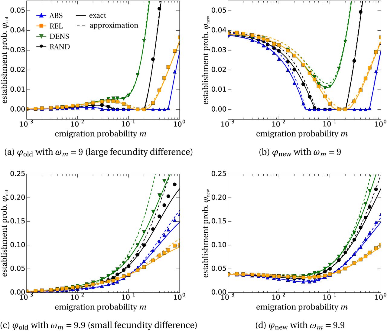
We plot the theoretical results for φold (panels (a) and (c)) and for φnew (panels (b) and (d)) for ωm = 9 in (a), (b) and ωm = 9.9 in (c), (d). Comparison with the results from stochastic simulations show very good agreement with our approximation found in eq. (7) (dashed lines). The solid lines are the numerical solution of eq. (6).
3 Results
We investigate the effect of the different dispersal schemes on the probability of successful adaptation and evolutionary rescue. We first compute the establishment probability of a single mutant individual arising either in an old- or in a new-habitat patch. We then link this probability to the dynamics of a source-sink system, i.e. a fixed environment with a certain number of old habitats (sources) and new-habitat patches (sinks). We derive an expression for the probability of a mutation to emerge and establish in a given time interval. We call this second quantity the probability of adaptation. Lastly, we study the time-varying scenario where patches, one after the other, deteriorate. We consider a third quantity, the probability of evolutionary rescue, which corresponds to the probability that a mutant appears by mutation and establishes in the new environment where all patches have deteriorated. The theoretical results are complemented by stochastic simulations that support our predictions and help visualize the differences between the different dispersal schemes.
3.1 Establishment probability in a heterogeneous environment
We derive the probability of establishment of a mutant population starting with a single mutant initially located either in an old- or a new-habitat patch. In this analysis, we ignore further mutations and are only concerned with the fate of this single mutant lineage. The dynamics of the mutant population can be described by a two-type branching process, i.e. all mutant individuals, descendants of the initial mutant, evolve independent of each other. This is a reasonable assumption as long as the overall number of mutants is a lot smaller than the population size of the wild type. The two “types” of the two-type branching process correspond to the two habitat types (old and new). The process tracks the numbers of old-habitat and new-habitat mutants,  with k denoting the habitat type (old or new). The number of offspring of a single mutant can be approximated by Poisson distributed numbers (see eqs. (2) and (3)). The mean number of offspring of a single mutant, either in an old- or a new-habitat patch, is then given by the following mean reproduction matrix:
 where the rows denote the parent locations, and the columns the patch type of the offspring. For example, the top-left entry reads as the probability for the parent to stay in an old-habitat patch
  times the average number of offspring in these patches, given by the mean of the corresponding Poisson distribution with rate (1+sold), cf. eq. (3). The other entries are obtained analogously.
The survival probability of this multi-type branching process, φk with k indicating the initial habitat type of the mutant, is then given by the unique positive solution of the following system of equations (see Haccou et al., 2005, Chapter 5.6)

A general analytical solution to these equations is not accessible, but the equations can be solved numerically. However, for weak selection and (potentially) weak dispersal – i.e. sold, snew, m « 1 needs to hold for at least two of the three parameters – an approximation is available: see for example Haccou et al. (2005, Theorem 5.6) for the general theory and Tomasini and Peischl (2018) for an application in a similar setting. The detailed derivation is presented in the Supplementary Information (SI), Section S2. We find
 where C is a scaling constant given by
 The first term in the approximation of the establishment probabilities (φold and φnew) in eq. (7) describes the local growth dependent on the habitat type under study. The second term denotes the effect of the heterogeneous environment that is most prominent for low to intermediate dispersal rates m; m is hidden in the constant C. Since C increases monotonically with increasing m, this term decreases for larger emigration rates. Biologically, the second term captures the growth rate differences between the two habitat types and corrects the local growth rate (first term) by the effect of dispersal events. The factor (1 − fold + πm fold) accounts for the biased dispersal patterns by increasing (decreasing) the importance of old-habitat patches for πm > 1 (πm < 1). The third term in the equations corresponds to the direct effect of dispersal on the establishment probability. The first two summands in the bracket are the same for both establishment probabilities. They represent the general effect of dispersal due to the dynamics from new-habitat patches (first summand) and old-habitat patches (second summand). Again, the dispersal bias induced by πm changes the relative impact of old- vs new-habitat patches. For higher values of πm, old-habitat patches have a stronger influence on the establishment dynamics of the mutant. Finally, the last summand in the bracket measures the growth rate loss (or gain) due to dispersal to the other patch type. It therefore differs between the two approximations.
Note that in these equations, the competition of the mutant with the wild-type in the old-habitat patches appears in the local growth rate sold, defined in eq. (2). This quantity is not constant, but instead depends on the wild type population size in old-habitat patches, which itself depends on the wild type’s dispersal and growth rate in both habitats.
If the emigration probability is zero (m = 0), the subpopulations in each habitat evolve in isolation from each other and we recover Haldane’s classical result for the establishment probability of a slightly advantageous mutant: φnew = 2snew (Haldane, 1927). Furthermore, in the case of random dispersal (πw = πm = 1) and for two patches, one exhibiting the old and one the new habitat (fold = 1/2), we obtain the approximation found in Tomasini and Peischl (2018) (compare system (7) to their eqs. (4) and (5)). Note, that the approximation is independent of the actual number of patches, but only depends on the environmental configuration determined by the frequency of old-habitat patches fold.
Comparison to simulations and qualitative behavior
In Figure 2 we compare our predictions from eqs. (6) and (7) to simulation results for different values of the emigration rate m. We find good agreement with the numerical solution of eq. (6 (solid lines) which justifies our Poisson reproduction assumption resulting in the mean reproduction matrix (see eq. (5)). The approximation from eq. (7) (dashed lines) deviates slightly from the simulation results in regions where m, snew and sold are not small, therefore violating the assumptions made in the analytical derivation.
The qualitative dependence of the establishment probabilities φold and φnew on the dispersal probability m is similar for all dispersal schemes. As visible, the shape of the curve strongly depends on the fecundity ωm of mutants in the old habitat. Before discussing the differences between the dispersal schemes, we first provide a qualitative understanding of this general behavior.
For the probability of establishment of a single mutant in an old-habitat patch (φold), we observe up to three different regions, cf. Figure 2(a). This is in line with previous observations in the context of local adaptation (e.g. Kawecki, 1995; Tomasini and Peischl, 2018) and evolutionary rescue (Uecker et al., 2014; Tomasini and Peischl, 2019). We define the regions as follows: (i) an initial increase of the establishment probability at low dispersal rates m; (ii) a local maximum with a subsequent decrease of the establishment probability; (iii) an increase of the establishment probability for high dispersal rates.
A detailed assessment and explanation of the regions is provided in the SI, Section S2.1. Briefly, in region (i) mutants disperse from old- to new-habitat patches where they are advantageous when compared to the wild-type, thus increasing the establishment probability. This effect is mediated through the third term of the establishment probability in eq. (7). Region (ii), beginning with the local maximum is dominated by the decreasing importance of locality due to larger dispersal rates, i.e. the population starts to homogenize over space. Quantitatively this means that the second term in eq. (7) is decreasing which causes the overall decline of the establishment probability. Finally, in region (iii) dispersal is so large that the population mixes very strongly. This culminates in less competitive pressure in old-habitat patches. Eventually, this yields a positive growth rate sold (first term in eq. (7)), responsible for the increase of the establishment probability in this region.
The width of the region of relaxed competition (region (iii)) strongly depends on the fecundity of the mutant in the old habitat, ωm. If ωm is high, the local growth rate of the mutant sold starts to increase for lower dispersal rates, see SI, Figure S1. This can cause region (ii) to completely vanish, as visible in Figure 2(c). On the other hand, for low mutant fecundity values ωm region (iii) might disappear as well, see Figure S2 in SI. There, the mutant is strongly disadvantageous in old-habitat patches when compared to the wild type, and the wild-type population will always outcompete the mutants due to the much higher offspring numbers.
We analyze the qualitative behavior of the establishment probability of a mutant emerging in the new habitat (φnew) (Figures 2(b,d)) in a similar way. Instead of an initial increase as observed for φold, the establishment probability φnew decreases for low dispersal rates. Since we let the mutant start in a new-habitat patch, where it fares better than the wild type, there is no initial benefit due to dispersal. Dispersal displaces the mutant from new- to old-habitat patches, thus the decline. The interpretation of regions (ii) and (iii), describing the trajectory for intermediate and large emigration rates m, is the same as for φold above.
Comparison of dispersal schemes
We now turn to the discussion of how the establishment probabilities compare for the various dispersal schemes. We consistently observe that negative density-dependent dispersal (green curves and triangles in Figure 2) acts as an enhancer of establishment when compared to the random dispersal scheme (black curves and circles). This can be attributed to two reasons: (1) the mutant is more likely to disperse to the new habitat where it outcompetes the wild type (stronger weighting of new-habitat patches in term (3) eq. (7)); (2) since the wild type prefers to settle in new-habitat patches (πw < 1), individuals in old-habitat patches experience relaxed competition for lower dispersal rates m thus increasing the local growth rate sold, i.e. region (iii) is shifted to the left. An analogous (but reversed) argument explains why absolute habitat choice (blue curves and upward triangles in Figure 2) is always lower than the random dispersal scheme (black curves and circles).
The effect of relative habitat choice (orange curves and squares in Figure 2), where each type has a bias to move to the habitat where it is relatively fitter than the other type, is more involved. We disentangle the effects separately for each region. In region (i) at low emigration probabilities, the curve is almost identical to that of the negative density-dependent pattern. The mutant preference of these two dispersal modes is the same. Since the movement of the rare mutants is governing this parameter regime, this explains the alignment of the green and the orange curves. For intermediate dispersal rates, the effect of the heterogeneous environment, term (2) in eq. (7), becomes stronger, i.e. the local growth rate sold increases because of relaxed competition in old-habitat patches. For relative habitat choice, the wild type is more likely to re-immigrate into old-habitat patches and by that increases the population size in these locations. This reduces the effect of relaxed competition. Therefore, the orange line now drops below the green curve and even starts to decrease, Figure 2(a). For high emigration probabilities m, region (iii), the competitive pressure in old-habitat patches relaxes. Again, this region is dominated by the movement of wild-type individuals. In the random dispersal scheme (black) the wild type has a lower likelihood to be in old-habitat patches than with the relative habitat choice scheme (orange), thus the black is above the orange line. For very large dispersal rates, also the absolute habitat choice scheme (blue curve) can predict higher values for φold than relative habitat choice (orange), cf. Figure 2(c). In this parameter regime, the mutant has a larger growth rate in old- than in the new-habitat patches (sold > snew). Therefore, it is beneficial for the mutant to stay or to re-immigrate into old-habitat patches.
3.2 Probability of adaptation in a heterogeneous environment
We now study the probability of adaptation, when mutations occur recurrently. As in the previous section, we consider a heterogeneous environment with a fixed number of old- and new-habitat patches. This is effectively a source-sink system (Holt, 1985; Pulliam, 1988), where old- and new-habitat patches correspond to sources and sinks for the wild type, respectively. In the previous section, we initialized the system with one mutant in either an old- or a new-habitat patch and computed the establishment probability. Now, we let mutants appear randomly within a certain time frame. We denote the last time point at which a mutation can occur by tfin. Later, in the analysis of the probability for evolutionary rescue this time will be replaced by the time between two consecutive patch deterioration events, τ. For now we will set this value arbitrarily to 100 and initialize the system with a fixed number of old-habitat patches.
The probability of adaptation in this setting, Padapt, is given by
 In words, this is one minus the probability of no mutant establishing within the [0, tfin] time interval. More precisely, the exponential is the probability of zero successes of a Poisson distribution. The rate of this Poisson distribution is given by the expected number of successfully emerging mutant lineages until time tfin. For tfin tending to infinity there will almost surely be a successful mutant so that Padapt = 1. For finite values of tfin the average number of mutations that appear until that time is given by the product of the mutation rate θ, the length of the time window of interest tfin, the number of patches M and the stationary number of wild-type individuals present in the different habitats, that is K and
  for old- and new-habitat patches, respectively (cf. SI eq. (S5)). Once such a mutant appears, it then has the previously computed establishment probability φk to establish, dependent on the patch type k (old or new) it arises in. This explains the factor φk in the exponential.
In Figure 3 we compare our prediction to simulation results. When varying the emigration probability m, we see that the shape of the probability of adaptation depends on the fecundity of the mutant in old-habitat patches, ωm (Figures 3(a,c)). This is similar to the behavior of the establishment probability φold in Figure 2. Likewise, the qualitative effects of the different dispersal schemes are comparable to the ones observed for the establishment probability.

In panels (a) and (c), we vary the emigration rate m and observe a similar qualitative behavior as for the establishment probability φk in Figure 2. In panels (b) and (d), we vary the frequency of old-habitat patches. The maximum is the result of two counteracting processes. The higher the number of old-habitat patches (i.e. the greater fold), the larger the wild-type population. As a consequence, more mutants appear in the studied time-frame. In contrast, the less old-patch habitats there are in the environment (i.e. the lower fold), the higher the probability of successful establishment of a mutant population. In all subfigures, the mutation rate is set to u = 1/(MK) and the considered time-window for a mutant to appear is set to tfin = 100.
In subfigures (b) and (d) we vary the frequency of old-habitat patches fold. We observe a maximum which is the result of two effects: (i) the likelihood for a mutation to appear increases with the number of wild-type individuals present in the system, which is highest for high frequencies of old-habitat patches fold, and (ii) the probability of establishment of a mutant decreases with the number of old-habitat patches.
The different dispersal schemes affect both effects. Negative density-dependent dispersal (green), when compared to random dispersal (black), always shifts the maximum to higher frequencies of old habitats while also increasing its quantitative value. Under negative density-dependent dispersal, mutant and wild-type individuals prefer settling in new-habitat patches (πw, πm < 1). As a result, the local population before reproduction in these patches is increased, so that the overall population size is higher compared to the other dispersal schemes. There is therefore a higher number of mutants generated under this scheme. Additionally, the probability of establishment is also increased for negative density-dependent dispersal, further increasing the probability of adaptation (see also the discussion around Figure 2). Again, a reversed argument explains why absolute habitat choice (blue) always yields lower probabilities of adaptation than random dispersal.
3.3 Habitat of origin of the adaptive mutation
We now identify the habitat type where the successful mutation arises. The established mutant population can arise from a mutant that is born in an old- or in a new-habitat patch, but can also be traced back to two (or more) mutant individuals, one from either patch type. For example, the approximation for the probability to observe a mutant population that can be traced back to a mutant from an old-habitat patch is the following

The corresponding probabilities for the other two scenarios can be computed analogously.
In Figure 4 we compare simulation results with our predictions for the origin of a successful mutant when varying the old habitat frequency fold. Surprisingly, even for a relatively strong fecundity disadvantage of the mutant in the old habitat, i.e. ωm is 10% smaller than ωw, we find that most successful mutations arise in old-habitat patches, subfigure 4(a). Decreasing the fecundity disadvantage of the mutant by increasing its fecundity ωm further increases the number of successful mutant lineages from old-habitat patches, subfigure 4(b). On the other hand, if we increase the fecundity difference in old habitats by decreasing ωm, we observe the inverse, i.e. eventually the probability for a successful mutation to arise in new-habitat patches becomes largest (see Figure S3 in SI).

The origin of the adaptive mutant is strongly affected by the fecundity differences in the old habitat. If the difference is large as illustrated in panel (a), mutants appear more often in old-habitat patches than in new-habitat patches. Still, mutants arising in new-habitat patches contribute to the overall probability of adaptation. If fecundity differences are small like in panel (b), the successful mutant largely arises in old-habitat patches. In this case, the contribution from new-habitat patches is negligible. Data points for at least two successful lineages, one arising in an old- and one in a new-habitat patch (circles) represent the simulations where both lineages are still present after 1000 generations. Note the different scalings on the y-axis.
3.4 Evolutionary rescue
Finally, we consider a time-inhomogeneous environment where patches deteriorate one after the other at regular time intervals τ, until all patches have switched to the new habitat. If the wild-type population fails to generate a successful mutant, the population will unevitably go extinct. Therefore, the probability of evolutionary rescue is tightly linked to the probabilities of adaptation and establishment which we have computed in eqs. (7) and (9). We approximate the probability for evolutionary rescue, denoted by Prescue, as
 where fold(i) = (M −i)/M is the frequency of old-habitat patches after the i−th deterioration event and
  denotes the overall number of wild-type individuals living in habitat k (old or new) in generation j. The intuition for the form of this equation is the same as for eq. (9).
As visible in Figure 5, the approximation matches the qualitative pattern of the simulation results, i.e. the ranking and intersection of the dispersal schemes. Yet, it does not accurately predict the simulated data. This discrepancy can be explained: in the formula we assume a constant establishment probability between two deterioration events. However, mutants that arise very shortly before a deterioration event just need to survive until this event happens and are thus carried over to the following environmental configuration with a higher probability than predicted by our formula. This explains why the real rescue probability is higher than our approximation, which ignores these “left-over” mutants present prior to the deterioration event. As a result, instead of assuming a constant establishment probability between two deterioration events, we would rather need a time-dependent establishment probability which cannot be approximated in our general framework (but see Uecker et al. (2014) where scenarios with an accessible time-dependent solution are studied).

Our predictions match the qualitative behavior of the simulated data for the probability of evolutionary rescue. All intersections and rankings of the dispersal schemes align well. Quantitatively though, we find that our predictions tend to underestimate the simulated data. In (a,b) the mutation rate is set to u = 1/(25MK) while in (c,d) it is u = 1/(MK).
Comparing the different dispersal schemes with each other, we see substantial affect the dispersal pattern of both types and as such alter their respective population dynamics. For both, small and large fecundity differences in the old habitat, ωm = 9.9 and ωm = 9, we see that the ranking and intersection of dispersal schemes is the same as for the probabilities of establishment and adaptation: from highest to lowest we have negative density-dependent (green), random dispersal (black), absolute habitat choice (blue) and intersections for the curve for relative habitat choice (orange), cf. Figure 5(a,b). Based on our discussion of the same behavior in Figure 2(a,c), this indicates that in these parameter sets the most influential factor is the growth rate of the mutant in old-habitat patches, sold.
For very large fecundity differences (ωm = 3 and ωm = 0), the intersections between relative habitat choice (orange) and the random dispersal scheme (black) and absolute habitat choice (blue) vanish, cf. Figure 5(c,d). In this parameter setting the probability of evolutionary rescue is dominated by the dispersal behavior of the mutant. Since the mutant is barely viable in old-habitat patches, it is always preferential for it to disperse towards new-habitat patches. The difference between negative density-dependent dispersal (green) and relative habitat choice can be traced back to the overall population size during the degradation process. Since wild-types also preferentially disperse to new-habitat patches under density-dependent dispersal, more individuals are present in those patches. This increases the total amount of mutations over the deterioration time, implying more chances for a mutant lineage to survive. This effect is even stronger for large dispersal rates that increase the wild-type population size in the whole environment. Together with the effect of relaxed competition, this explains the strong increase of the negative density-dependent and the random dispersal scheme in Figure 5(c).
Lastly, we see that the probability of evolutionary rescue reaches a local (or global) maximum for intermediate emigration probabilities, subfigures 5(c,d). This recovers previous results (Uecker et al., 2014; Tomasini and Peischl, 2019). The maximum can be attributed to the interaction of the three regions we identified when analyzing the establishment probability φk (see also Figure 2). As such it is a result of the largely positive effect of dispersal (initial increase of the probability of evolutionary rescue) and the negative effect of population mixing and reduced habitat differences (see the second term in eq. (7) and the discussion of region (ii) in the same section).
3.5 Habitat of origin of the rescue mutant and standing genetic variation
Concerning the habitat type of the origin of the successful mutant lineage that eventually rescues the population, we find that the rescue mutant mostly arises in old-habitat patches (acting as sources). More individuals are available for a mutation to appear in these patches than in new-habitat patches. The amount of successful mutants appearing in old-habitat patches decreases when ωm decreases (compare black and yellow symbols in Figure 6(a)). This shows that for smaller fecundity values ωm the probability for the rescue mutation to appear in the already deteriorated habitat, i.e. in new-habitat patches, increases.

(a) We compare the source of successful mutations under small (black) and large (yellow) fecundity differences in the old habitat. Decreasing the fecundity of the mutant results in more successful mutations emerging in new-habitat patches (+) while the contribution to the rescue probability from old-habitat patches (×) decreases. We have chosen πm = πw = 1. (b) We observe that for slower environmental degradation, i.e. increasing values of τ, the influence of standing genetic variation (sgv) on the probability for evolutionary rescue decreases. The simulations are done by letting the system evolve for 1000 generations before the first deterioration event happens. Further, πm = πw = 1 in all scenarios and ωm = 9.9. The relative contribution is then determined by (Prescue with sgv − Prescue only de novo)/Prescue with sgv.
In Figure 6(b) we explore the effect of standing genetic variation on the process of evolutionary rescue. Typically, in formulas expressing the probability of evolutionary rescue, one splits the contributions into mutations arising de-novo, i.e. after the environment deteriorated, and evolutionary rescue due to standing genetic variation, i.e. mutations that are present in the population before the environmental change (Alexander et al., 2014). In our default parameter set where the environmental change lasts for 900 generations (= (M − 1)τ), contributions due to standing genetic variation, i.e. mutants that were present before the first patch deteriorates, are small (circles in Figure 6(b)).
Additionally, we observe a decline of relative contribution of standing genetic variation as the emigration rate m increases. This is explained by the homogenizing effect of large dispersal rates. Both, for small and large fecundity differences in the old habitat, the homogenization results in purging the mutant more quickly. This holds because it has no chance to establish for large frequencies of old-habitat patches fold (see again Figures 3(b,d) where m = 0.06 (for larger emigration rates see Figure S4 in SI)). Thus, mutants that existed prior to the first deterioration event are very unlikely to survive even for a rapidly changing environment. Therefore, no or only very few successful mutant lineages are generated from standing genetic variation.
4 Discussion
We have studied the probabilities of establishment, adaptation and evolutionary rescue under three non-random dispersal schemes and compared them to random dispersal. Our analysis builds on the probability of establishment of a single mutant lineage in a heterogeneous environment with a fixed patch configuration. In line with previous results, we find that the probabilities of establishment, adaptation and evolutionary rescue can display up to three different phases when varying the dispersal rate m: Increasing with dispersal at low dispersal rates the establishment probability increases, decreases at intermediate dispersal rates, and restarts increasing at large dispersal rates. The different dispersal schemes, by changing the population dynamics, broaden, tighten or shift these regions.
4.1 Dispersal and adaptation
Theoretical studies that investigated the effects of spatial subdivision on the adaptation of a population in a heterogeneous environment can be classified into two types. One type of models, classically analyzed in a population genetic context, assumes constant population sizes in all patches, independent of their local habitat type and of dispersal strength. Results obtained in this framework show that larger dispersal rates tend to decrease the probability of successful establishment of a rare mutant favored in some part of the environment (e.g. García-Ramos and Kirkpatrick, 1997). This inhibiting effect of dispersal on adaptation, also termed “gene swamping”, is a result of an increase in absolute numbers of non-adapted individuals in the habitat where the rare mutant is beneficial, resulting in a lower mutant frequency (Lenormand, 2002; Tomasini and Peischl, 2018). Additionally, for very high dispersal rates, the population homogenizes and individuals encounter an averaged environment. Therefore, the type with the largest overall growth rate, averaged over the environment, is favored.
The second type of models explicitly takes into account demographic effects due to dispersal, often resulting in source-sink dynamics (Holt, 1985; Pulliam, 1988). Here, the effect of dispersal on adaptation depends on the growth rate differences of the mutant and the wild type in the two habitats (Kawecki, 2000). In accordance with this result, we find that dispersal increases the probability of adaptation if the mutant is just slightly less fit than the wild type in the old habitat, ωm = 9.9 (Figure 2(c,d)). We observe non-monotonic establishment probabilities with a local maximum at intermediate dispersal rates when increasing the disadvantage of the mutant in old-habitat patches, i.e. decreasing its fecundity ωm, see Figure 2(a). For large emigration rates m the probability of establishment increases again – a result of the alleviated competitive pressure in old-habitat patches. If we further increase the mutant disadvantage (i.e., decrease ωm, adaptation is also hindered for large dispersal rates. The establishment probability becomes hump-shaped (cf. Figure S2 in SI). This is explained by adapted mutants immediately being purged in old-habitat patches. For large dispersal rates, the fecundity disadvantage of the mutant is too large for it to profit from the relaxed competition in old-habitat patches. Therefore, no final increase in the establishment probability is observed.
The striking qualitative difference between models with and without demographic changes is region (iii) where relaxed competition in old-habitat patches is the dominating factor. In models without demography, population sizes in both patch types are at carrying capacity. Therefore, the effect of relaxed competition is negligible in these type of models producing hump-shaped probabilities of establishment and adaptation, see Figure S5 in SI. In contrast, we find that relaxed competition explains the dynamics of adaptation for large dispersal rates in models that take into account demographic changes.
4.2 Dispersal and evolutionary rescue
The qualitative behavior of the probability of evolutionary rescue under variation of the dispersal rate m can largely be explained by our reasoning for the probability of adaptation. Again the variation of the mutant fecundity in the old habitat, ωm, determines the shape of the curve in our model, see Figure 5. This recovers the results obtained by Uecker et al. (2014), where the effect of random dispersal on evolutionary rescue was studied. Recently, Tomasini and Peischl (2019) derived a condition for when evolutionary rescue gets promoted by dispersal. We extend these two studies by exploring the effect of different dispersal schemes and investigating the habitat type of the origin of the rescue mutation as well as the impact of standing genetic variation before the first patch deteriorates.
The strength of the fecundity disadvantage of the mutant in old-habitat patches, sold, determines whether the population is primarily rescued from mutants arising in old- or in new-habitat patches (Figure 4 and Figure 6(a)). Larger disadvantages, i.e. lower values of ωm, culminate in a larger proportion of successful rescue mutations from the new habitat. This seems reasonable since survival of arising mutants in old-habitat patches is reduced (compare also Figures 2(a) and (c)).
The impact of standing genetic variation on the overall probability of evolutionary rescue increases with the speed of the environmental change determined by τ, Figure 6(b). This observation has also been found in a quantitative genetics setting where the adaptive trait is continuous (and not discrete as in our model). Experimental results with Caenorhabditis elegans indicate that under slow environmental change the impact of standing genetic variation is small (Guzella et al., 2018). This is because the evolution of the trait is driven by de novo mutations with small effects. For a sudden or fast environmental change however (small τ), standing genetic variation becomes increasingly important for the probability of evolutionary rescue. These observations are in line with our findings in Figure 6(b) and other theoretical results obtained in this context (Matuszewski et al., 2015).
4.3 The effect of different dispersal patterns on adaptation and evolutionary rescue
The importance of dispersal schemes different from random dispersal has been highlighted recently (Edelaar et al., 2008; Clobert et al., 2009; Edelaar and Bolnick, 2012). This led to a number of simulation studies exploring the effects of various dispersal schemes onto adaptation and niche width (Vuilleumier et al., 2010; Holt and Barfield, 2015; Mortier et al., 2018; Pellerin et al., 2018).
Two of these simulation studies examined the effects of matching habitat choice on adaptation to a heterogeneous environment (Vuilleumier et al., 2010; Holt and Barfield, 2015). Both investigations indicate that matching habitat choice increases the probability of adaptation when compared to random dispersal. This is in line with our findings: we predict that type-dependent habitat choice (orange lines) generates higher probabilities of establishment and evolutionary rescue than random dispersal (black lines), Figures 2, 3, 5.
As already discussed, these observations are largely driven by the comparison of the local growth rates, sold and snew, which becomes apparent when looking at eq. (7). The effect of different dispersal schemes can be predicted by their corresponding effects on these two values. Since density regulation in the new habitat is not relevant, due to a declining population in these patches, snew is not affected by the dispersal schemes. In contrast, the growth rate in the old habitat, sold, depends on the number of wild-type individuals after dispersal,  (see eq. (2)). This number varies strongly for the different dispersal schemes. Thus, in our model, the dispersal scheme that maximizes the average number of offspring of a single mutant individual in the old habitat will also promote establishment, adaptation and evolutionary rescue the strongest. This observation explains why negative density-dependent dispersal (green lines), by alleviating competition and increasing the wild type population the most, always has the highest corresponding probabilities. Interestingly, for large dispersal rates m this is also the reason why relative habitat choice (orange) will not always result in higher probabilities than random dispersal (black); see for example Figure 2(a,c). If fecundity differences between the mutant and the wild type in the old habitat are small, the growth rate of the mutant in these patches is higher than in new-habitat patches, i.e. sold > snew. Therefore it is beneficial to the mutant to preferentially immigrate into old-habitat patches, explaining why for these parameters random dispersal performs better than relative habitat choice.
Lastly, the dispersal schemes also affect the origin of the successful mutant lineage. Population densities, especially in new-habitat patches, are altered when compared to the random dispersal scheme. However, this has only a minor impact on the habitat type of the origin of the rescue mutation, cf. SI, Figure S6.
In summary, the effects of dispersal schemes are two-fold. By changing population densities in both habitat types, the dispersal schemes change the growth rate of the mutant in old-habitat patches. This is the primary reason for the ranking of the dispersal schemes. In addition, they also affect the number of mutations arising in either habitat type. This has a minor effect on the probability of evolutionary rescue but is relevant when studying the origin of the successful mutant lineage.
4.4 Evolutionary consequences of habitat choice
The interplay of local adaptation and habitat choice has interested evolutionary ecologists for several decades, see for example Rosenzweig (1981) for one of the first references. In our study we are interested in the effect of habitat choice and density-dependent dispersal on the establishment of a newly arising type and on the probability of evolutionary rescue.
Our analysis shows that both quantities are suppressed under absolute habitat choice; see blue lines in Figures 2 and 5. This indicates that habitat choice protects a population against locally deleterious mutations if the mutant has the same dispersal pattern as the wild type, i.e. πm = πw > 1. This is achieved by maintaining a large local density in old-habitat patches which increases the local selection strength. Therefore, fecundity differences between the mutant and the wild type have a strong impact on the composition of the next generation.
In a scenario where habitat choice and adaptation to the habitat are two independent traits, the adaptive mutant will share the habitat preference of the wild type at its emergence. For strong habitat preferences (large πw) this can result in new patches remaining empty. This observation was also made in Ravigné et al. (2009) – even though in a different model not exhibiting source-sink dynamics and under a different regulation scheme. In that study the authors analyzed the co-evolution of a habitat choice trait and a local adaptation trait. In their “model 1” that is closest to our life cycle, if habitat choice is fixed and only the adaptive trait evolves, the results depend on the difference of the growth rates in the two habitats. If differences are small, a generalist evolves while for large differences one specialist emerges, leaving one of the habitats empty. The latter situation would correspond to the absolute habitat choice dispersal scheme. In the scenario where the two traits co-evolve, the authors predict evolutionary branching, i.e. the coexistence of two specialist types with their own habitat preference. This relates to our relative habitat choice scenario (orange). For low to intermediate dispersal rates and under large fecundity differences, relative habitat choice yields higher probabilities for establishment than random dispersal. Therefore, if a mutant is able to quickly evolve its own habitat preference, it has an increased chance of establishing in the meta-population. This is in agreement with recent experimental findings in the ciliate T. thermophila (Jacob et al., 2017). Even though we do not explicitly consider speciation and the evolution of genetic polymorphisms, our results suggest that type-dependent matching habitat choice enhances segregation. This follows from the probability of adaptation for relative habitat choice (orange) being higher than for absolute habitat choice (blue) or random dispersal (black), Figure 3. This idea has already been promoted in other theoretical and experimental studies (e.g. Rosenzweig, 1987; Rice and Salt, 1990; Ravigné et al., 2009; Jacob et al., 2018).
4.5 Generality of our theoretical analysis and future directions
Our mathematical results apply in the general case where the mutant offspring numbers can be written in the form “migration times reproduction (and potential regulation)” with rates that are constant in time, see the mean reproduction matrix in eq. (5). Biologically this means that the resident population is in stationarity and the mutant is either at low numbers or unaffected by its own density. Furthermore, for our approximation in eq. (7) to generate accurate predictions, it is essential that growth rate differences between the wild type and the mutant are weak and dispersal is low. Formally, just two of these parameters need to be small, see also the corresponding discussion in Tomasini and Peischl (2018).
Since we summarize the population dynamics in our parameters of the reproduction matrix the approach taken here is quite general and can account for various dispersal schemes and local population dynamics. However, it cannot account for spatial structure as for example the stepping stone model. Further it also fails to account for time-inhomogeneous environments. This is the reason for our approximation to perform worse in the context of evolutionary rescue (Figure 5). Additionally, in order to obtain analytical solutions it is important that the stationary population sizes of the wild type have an accessible solution. This is not the case if for example we consider non-linear emigration rates that depend on habitat choice like incorporated in some simulation studies (e.g Holt and Barfield, 2015; Mortier et al., 2018).
In contrast, it should be possible to include a cost of dispersal and a different life cycle. Especially the variation of the life cycle could yield qualitatively different results regarding adaptation (Holt and Barfield, 2015) and more generally in the context of evolution of dispersal (Massol and Débarre, 2015).
In conclusion, we studied the effect of dispersal and different dispersal schemes on the probability of establishment, adaptation and evolutionary rescue of a mutant under divergent selection in a heterogeneous environment. Our quantitative approach disentangles the inter-action of dispersal and adaptation. We recover previous results on adaptation and identify the forces that are responsible for the different predictions obtained in different biological communities. Most importantly, we find that including population demography significantly alters the results for high dispersal rates. For constant population sizes high dispersal rates have a negative effect on establishment, while under population size changes the effect is largely positive. The latter is a result of relaxed competition in old-habitat patches. Most importantly, we extend the existing literature by comparing different dispersal schemes and studying their effects on adaptation and evolutionary rescue. Our results indicate that habitat choice does not necessarily result in an increased adaptive potential and might even hinder successful establishment of a mutant population that would prevent the population to become extinct. Negative density-dependent dispersal on the other hand, always increases the probability of adaptation and evolutionary rescue. These results show that non-random dispersal patterns can have a strong influence on population survival and adaptation in a heterogeneous environment. This type of eco-evolutionary considerations is especially important in times of environmental change and biodiversity loss (Thompson and Fronhofer, 2019).
Acknowledgements
PC and FD received funding from the Agence Nationale de la Recherche, grant number ANR-14-ACHN-0003-01. HU appreciates generous funding from the Max Planck Society.


