

Abstract
Inferring gene trees is difficult because alignments are often too short, and thus contain insufficient signal, while substitution models inevitably fail to capture the complexity of the evolutionary processes. To overcome these challenges species tree-aware methods seek to use information from a putative species tree. However, there are few methods available that implement a full likelihood framework or account for horizontal gene transfers. Furthermore, these methods often require expensive data pre-processing (e.g., computing bootstrap trees), and rely on approximations and heuristics that limit the exploration of tree space. Here we present GeneRax, the first maximum likelihood species tree-aware gene tree inference software. It simultaneously accounts for substitutions at the sequence level and gene level events, such as duplication, transfer and loss and uses established maximum likelihood optimization algorithms. GeneRax can infer rooted gene trees for an arbitrary number of gene families, directly from the per-gene sequence alignments and a rooted, but undated, species tree. We show that compared to competing tools, on simulated data GeneRax infers trees that are the closest to the true tree in 90% of the simulations in terms relative Robinson-Foulds distance. While, on empirical datasets, GeneRax is the fastest among all tested methods when starting from aligned sequences, and that it infers trees with the highest likelihood score, based on our model. GeneRax completed tree inferences and reconciliations for 1099 Cyanobacteria families in eight minutes on 512 CPU cores. Thus, its advanced parallelization scheme enables large-scale analyses. GeneRax is available under GNU GPL at https://github.com/BenoitMorel/GeneRax.
Introduction
Reconstructing the evolutionary history of homologous genes is a fundamental problem in phylogenetics, as gene trees play a prominent role in numerous biological studies. For instance, gene trees are essential to understand genome dynamics (Touchon et al., 2009), to study specific traits (Musilova et al., 2019), or to infer the species tree (Boussau et al., 2012; Mirarab et al., 2014).
Most common methods infer phylogenetic trees from multiple sequence alignments (MSAs), for instance using the maximum likelihood (ML) criterion (Kozlov et al., 2019; Nguyen et al., 2015). Under the correct substitution model, ML methods are statistically consistent (Yang, 1994), that is, they converge to the true tree when the sequences are long enough. However, this condition is often violated for gene trees: typical per-gene MSAs are short (50 to 1000 sites) and can comprise a large number of sequences representing a large number of taxa (hundreds or thousands for large gene families). As a result, there is typically insufficient signal in the MSA to reconstruct a well supported phylogeny. In other words, the tree with the highest likelihood will most likely not correspond to the true tree.
Species-tree-aware (STA) approaches aim to compensate for this insufficient signal by relying on a putative species tree. Indeed, gene trees and the species tree exhibit an intricate relationship: genes evolve within a (species) genome and undergo biological processes such as duplication, horizontal gene transfer (HGT), loss, or speciation (Fig. 1). Therefore, although gene trees can be topologically different from the species tree, their own evolutionary history is greatly affected by the species tree. STA methods use this dependence between the gene trees and the species tree as additional information to either directly infer or a posteriori correct gene trees. In the following, we denote gene duplication, gene loss, and horizontal gene transfer events as DTL events.
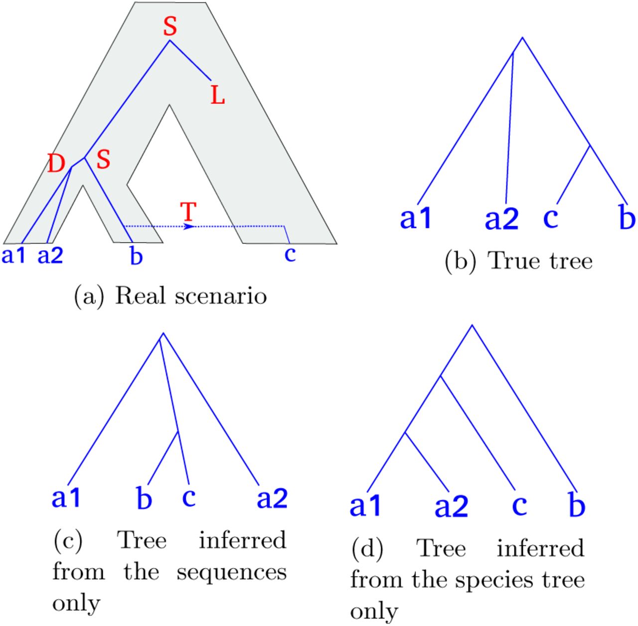
A gene tree evolving along the species tree, and several possible inferred trees. (a) The true history. The gene tree (blue lines) evolves within the species tree (grey area), and undergoes speciations (S), duplications (D), losses (L) and HGT (T). (b) The true gene tree. (c) A gene tree inferred with a sequence-aware method. The duplication and the speciation between the species a and b are very close in time, and there is not enough signal in the sequences to correctly decide which split happened first. (d) Tree inferred from the species tree only (without accounting for the sequences), assuming that HGT are less likely than duplications.
A common approach used by STA methods (Chen et al., 2000; Noutahi et al., 2016; Scornavacca et al., 2014) consists in contracting weakly supported gene tree branches into polytomies, which are subsequently resolved using the species tree. This heuristic limits the set of gene trees explored to trees that can be obtained as combinations of alternative resolutions of the contracted branches, and in most existing implementations (Chen et al., 2000; Noutahi et al., 2016) based on parsimony requires arbitrary DTL parsimony costs. This is especially problematic if the substitution model is miss-specified, or fails to adequately capture the complexity of the data (which if often the case for shorter gene alignments where parameter rich substitution models are more difficult to use). In addition, the user must define what a “weak support value” is, often by setting an arbitrary threshold. Treerecs (Comte et al., 2018) addresses this last limitation by exploring several thresholds, and returning the gene tree that maximizes a likelihood score that is based on both, the MSAs and the species tree. Finally, obtaining branch support values usually requires a significant amount of computational effort (e.g., 1-2 orders of magnitude more than for a simple ML tree search on the original MSA, if the classic Felsenstein Bootstrap is used (Felsenstein, 1985)).
Other STA methods utilize a hierarchical probabilistic model of sequence level substitutions and gene level events, such as duplication, transfer and loss. This allows the definition of the joint likelihood as the product of the probability of observing the alignments given the gene trees (phylogenetic likelihood) and the probability of observing the gene trees given the species tree (reconciliation likelihood):
 where S is the species tree, 𝒢 is the set of gene trees, and 𝒜 the set of MSAs. Phyldog (Boussau et al., 2012) co-estimates the gene trees and the species tree by conducting a tree search that is based on such a joint likelihood score. However, Phyldog does not model HGT. ALE (Szöllősi et al., 2013a) calculates the joint likelihood using a dynamic programming scheme that requires the phylogenetic likelihood to be approximated by conditional clade probabilities (Larget, 2013). In order to calculate conditional clade probabilities ALE requires a sample of gene trees as input that are typically obtained via Markov Chain Monte Carlo (MCMC) sampling. This approach has two shortcomings, first the conditional clade probability approximation inevitably limits the set of gene trees explored to trees that are comprised of clades observed in an tree sample, as the phylogenetic likelihood of all other trees is approximated to be zero (Szöllősi et al., 2013a). While less severe, conceptually this limitation is similar to that exhibited by the branch contraction methods discussed above, and is similarly sensitive to model miss-specification and inadequacy. Second, obtaining a tree sample, either by running Bayesian phylogenetic MCMC methods or by using bootstrap methods for a set of gene families is computationally expensive. For an in depth review of gene tree inference methods, see (El-Mabrouk and Noutahi, 2019; Szöllősi et al., 2014).
Probabilistic frameworks to model both, sequence (Felsenstein, 1981), and gene evolution events (Åkerborg et al., 2009; Szöllősi et al., 2012a) can be found in the literature. However, at present, no ML tool is available that can directly infer gene trees from MSAs by simultaneously accounting for sequence substitutions and DTL events. We believe that such a method can significantly improve the accuracy of gene tree inference. A common argument against using STA ML approaches is the amount of time and computational resources required to conduct such an analysis (El-Mabrouk and Noutahi, 2019). However, a joint (phylogenetic and reconciliation likelihood) ML approach dispenses with the pre-processing steps required by other methods obsolete and can thereby decrease the overall computational cost significantly, while at the same time increasing accuracy. Tree search heuristics are widely used to infer trees from sequences only (Kozlov et al., 2019; Nguyen et al., 2015) using the phylogenetic likelihood. Thus, extending these methods by joint likelihood calculations represents a natural way of improving the accuracy of gene tree inference.
Here we introduce GeneRax, our novel software to infer reconciled gene trees via a joint ML tree search. The GeneRax input consists of a rooted, but undated binary (fully bifurcating) species tree, a set of per-family MSAs (DNA or amino-acid), and corresponding gene-to-species leaf name mappings. In addition, the user can provide initial gene family trees, typically inferred via non-STA methods (Kozlov et al., 2019; Nguyen et al., 2015). GeneRax is easy to use, models DTL events, and can process the gene families in parallel. Employing a hierarchical probabilistic model allows it to simultaneously account for both the signal from the gene family MSAs and from the species tree. It estimates all substitution and DTL event intensity parameters, and does not require any ad hoc threshold or set of DTL event parsimony costs.
New Approaches
In this section, we outline the joint likelihood computation, our tree search algorithm, and our parallelization scheme.
Reconciliation likelihood
In this subsection, we derive the reconciliation likelihood function for an undated rooted species tree and a rooted gene tree, as implemented in ALE.
The “undated” DTL model, in contrast to the continuous time model described in (Szöllősi et al., 2013b), is a discrete state model, which begins with a single gene copy on a branch of the species tree. Subsequently gene copies evolve independently until either all copies are observed at the leaves or every gene becomes extinct. On an arbitrary branch of the species tree a gene copy either duplicates (with probability pD), in which case it is replaced by two gene copies on the same branch, arrives via transfer (with probability pT), in which case a copy is left on the donor branch, is lost (with probability pL) or finally (with probability pS = 1−pD −pT − pL) either i) for internal branches, undergoes a speciation event, in which case it is replaced by a copy on each descendant branch or ii) for terminal branches arrives at the present and is observed, terminating the process.
We denote by δ, λ, and τ the duplication, loss, and transfer intensity parameters and parametrize the above event probabilities as follows:


Let e be branch of the species tree S, and let f and g be its descendant branches (remember that the species tree is rooted). Let 𝒯 (e) be the set of species tree branches that can receive a HGT from e. Because we do not assume any time information on the species tree aside of the order of descent implied by the tree topology, we consider that 𝒯 (e) corresponds to all nodes that are not ancestors of e. We allow transfers from e to its descendants, because a gene could have evolved along an extinct or unsampled lineage and have been transferred back to a descendant of e (Szöllősi et al., 2013b).
The probability that a gene copy observed on an internal branch e becomes extinct before the present is:

The terms correspond to respectively the i) probability of loss, ii) speciation and subsequent extinction in both descending lineages (this term must be omitted for terminal branches), iii) duplication and subsequent extinction of both copies and finally iv) transfer and subsequent extinction of both the donor copy on branch e and the transferred copy on branch h, were for the latter event we have introduced the notation:

In (6), the value of Ee depends on ĒT, and thus on the extinction probabilities of all the species in the species tree. We iteratively estimate ĒT and Ee for all node e in the species tree, by initializing [E e]0 = 0 and computing:

If the limit of the sequence [E e]n exists, then it is solution of (6). We do not prove here the existence of this limit.
We observed on simulations that 5 iterations are enough to estimate Ee, and we set the number of iterations to 5 in our implementation. In the special case where τ = 0 (no HGT), the term ĒT is equal to zero, and we can directly compute Ee from Ef and Eg.
To calculate the probability of a rooted gene tree G we have to sum over all reconciliations of G with S, i.e. all possible scenarios involving D, T, L and speciation events that may have produced the observed rooted gene tree topology along the species tree. To describe the sum over reconcilations, we begin with the probability Pe,u of observing some internal branch u of G on an internal branch e of S. Let v and w be the descendants of u on G and f and g be the descendants of e on S, we can write Pe,u as:
 were we have introduced the notation:
 and the terms on the right correspond to respectively i) speciation with both descending gene lineages surviving, ii) speciation and subsequent extinction (these term must be omitted for terminal branches), iii) duplication and subsequent extinction, iv) duplication and subsequent extinction of one of the copies and finally v) transfer with respectively branch v and w corresponding to the copy remaining in the donor linage, and finally vi) transfer and subsequent extinction of respectively the the donor or the recipient copy.
Pe,u depends on itself through the terms involving transfer where the recipient gene does not go extinct, we solve this through fixed point iteration analogously to (6). Aside of the self dependence, every other term involves either descendent branches in G (u and w), descendent branches in in S (f and g) or both, this allows us to set up a bottom-up dynamic programming recursion starting at the leaves, such that for leaf g of the gene tree and leaf s of the species tree P (g,s)= 1 if g gene maps to species s and zero otherwise.
Let G be a rooted gene tree, r its root, S a rooted species tree and N = {δ,τ,λ} the set of DTL intensity parameters. Then the reconciliation likelihood function is defined as:

Joint likelihood evaluation
GeneRax attempts to maximize the joint likelihood function defined as:
 where 𝒢 is the set of gene trees, S is the species tree, N are the DTL event intensity parameters, and 𝒜 is the set of gene MSAs.
GeneRax estimates the reconciliation likelihood L(S,N |Gi) based on the dynamics programming recursion described above. It uses the highly optimized pll-modules library (Darriba et al., 2019) to compute the phylogenetic likelihood L(Gi|Ai). Hence, GeneRax offers all substitution models supported by RAxML-NG (Kozlov et al., 2019).
Joint likelihood optimization
Given a set of MSAs and a species tree, GeneRax searches for the set of rooted gene trees and DTL intensity parameters that maximize the joint likelihood. We illustrate the search pipeline in Fig. 2.

GeneRax pipeline. In each step, we draw in red the parameters that GeneRax optimizes, and in grey the fixed parameters that GeneRax uses to compute the likelihoods. GeneRax performs Step 0 only when starting from random gene trees, to infer ML gene trees from the MSAs. Step 1 optimizes the DTL event rates from the gene trees and the species tree. Step 2 optimizes the gene trees from the MSAs, the species tree and the DTL rates. GeneRax repeats Step 1 and Step 2 with increasing SPR radius, until it reaches the maximum radius. Then it applies Step 3 to reconcile the gene trees with the species tree.
GeneRax either starts from user-specified gene trees or from random gene trees. Our joint likelihood search algorithm needs to start from gene trees with high phylogenetic likelihood, preferably inferred with phylogenetic ML tools such as RAxML-NG (Kozlov et al., 2019). We provide a rationale for this in the Results section. When starting from random gene trees, GeneRax performs an initial search (Step 0 in Fig. 2) to only maximize the phylogenetic likelihood, without accounting for the reconciliation likelihood.
After this optional step, GeneRax starts optimizing the joint likelihood, by alternatively optimizing the gene trees and the DTL event intensity parameters.
When optimizing the gene trees (Step 1 in Fig. 2), GeneRax processes each family independently, and applies a tree search heuristic to each of them separately: for a given tree, it tests all possible Subtree Prune and Regraft (SPR) moves within a given radius and then applies the SPR move that yields the tree with the best joint likelihood. Then it iterates by applying SPR moves on this new tree, until the joint likelihood can not be further improved. At the end of the gene tree optimization, GeneRax increases the SPR radius by one.
GeneRax optimizes the DTL intensity parameters globally over all gene families (Step 2 in Fig. 2). To this end, we apply the gradient descent method to find a set of DTL intensity parameters that maximizes the reconciliation likelihood over all gene families. We numerically approximate the gradient with finite differences.
The whole procedure stops when the SPR radius (starting from 1) exceeds a user-defined value. When the user does not define this maximum SPR radius, we set it to 5, as we did not observe any improvement above this value on our experiments.
Gene tree and species tree reconciliation
The reconciliation likelihood computation algorithm recursively traverses in post-order traversal both, the species tree, and the gene tree, and sums over all possible scenarios at each step of the recursion. To infer the ML reconciliation (Step 3 in Fig.2), GeneRax keeps track of the maximum likelihood path during the recursion.
GeneRax can export the reconciled trees into both Notung (Chen et al., 2000) and RecPhyloXML (Duchemin et al., 2018) formats (Fig. 3).
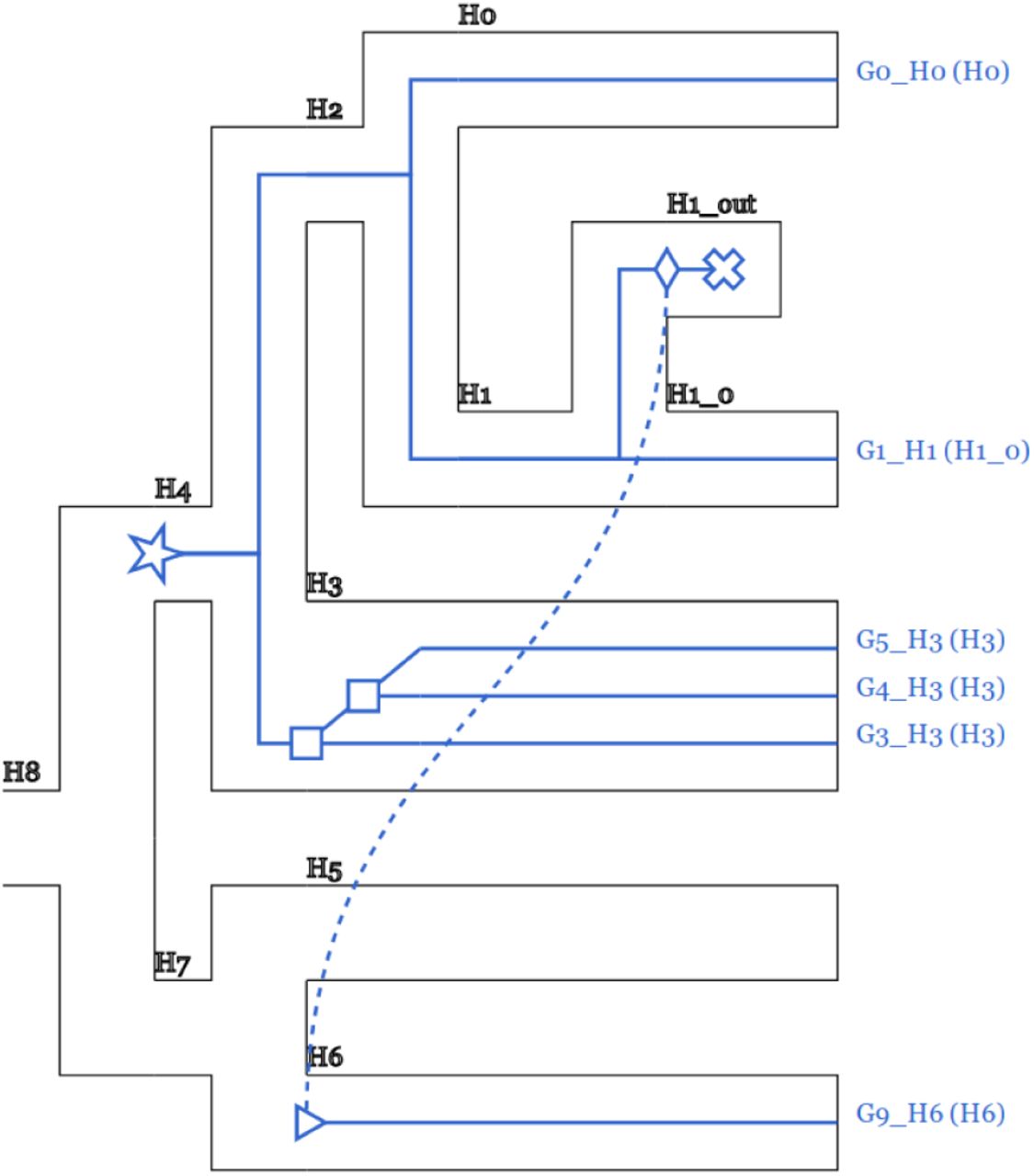
Reconciled gene tree and species tree. Users can easily visualize reconciliations inferred with GeneRax using the online tool RecPhyloXML-visu (Duchemin et al., 2018). This example illustrates one HGT and one duplication events.
Parallelization
Achieving ‘good’ parallel efficiency given a large number of gene families is challenging: the most natural solution consists in assigning a subset of gene families to each core (Boussau et al., 2012). However, gene family MSAs are highly heterogeneous in terms of size, and are hence hard to evenly distribute over cores (Morel et al., 2018) such as to achieve ‘good’ load balance. In particular, large gene family MSAs can easily generate a parallel performance bottleneck. Our solution allows to split up inferences on these large gene families across several cores. Thus, we parallelize over, but also within gene families, in analogy to our ParGenes (Morel et al., 2018) tool. However, unlike ParGenes, GeneRax parallelizes individual gene family tree searches over the possible SPR moves and not over MSA sites. This has two reasons: (1) the reconciliation likelihood computation does not depend on the number of sites (i.e., a parallelization will not scale with the number of sites in contrast to the phylogenetic likelihood), and (2) gene sequences are typically not long enough to efficiently parallelize phylogenetic likelihood calculations over the sites.
Experiments
We compared GeneRax to competing gene tree inference methods on both, simulated, and empirical datasets.
Tested software
This subsection describes the settings we used for executing the competing tools (summarized in Table 2) in all of our experiments.
Description of the empirical datasets used in our benchmarks. We extracted the Primates dataset from the release 96 of the Ensembl Compara database (Zerbino et al., 2017). The Cyanobacteria dataset was originally used in a previous study (Szöllősi et al., 2013a) and was extracted from the HOGENOM database (Penel et al., 2009).
Softwares used in our benchmark, with the type of method (ML, parsimony or both), the nature of the input trees (random tree, ML tree, tree with bootstrap support values or MCMC sample of trees), whether the method is STA and whether the method accounts for HGT.
We used ParGenes (Morel et al., 2018) to run RAxML-NG with 10 random and 10 parsimony starting trees and 100 bootstrap trees. For methods requiring starting gene trees, we selected the tree with the best likelihood found by RAxML-NG. We used 100 bootstrap trees to compute gene trees with branch support values as required for Notung and Treerecs. As Notung does not provide any clear recommendation for setting the bootstrap support threshold, we used the default value (90%). We executed Treerecs with its automatic threshold selection from seven threshold values (seven is the default value). We executed Phyldog with a fixed species tree. In the absence of recommendation, we set its maximum SPR radius to 5, as in GeneRax. To execute ALE, we first generated posterior tree samples with MrBayes, using two independent runs, four chains, 1,000,000 generations, a sampling frequency of 1,000 and a burn-in of 100 trees. We used the undated ALE model to produce 100 tree samples per gene family. We used the same MrBayes tree samples to execute EcceTERA with the amalgamate option, without transfer from the dead, and with the dated species tree option.
Note that, Treerecs, Notung, MrBayes, EcceTERA and ALE do not provide a way of parallelizing over gene families on cluster architectures. To execute them on large datasets, we scheduled them with an MPI program, by dynamically assigning jobs (with one job per gene family) to the available MPI ranks, starting from the most expensive jobs with the largest gene family MSAs. Henceforth, we refer to sequential runtime as the sum of the time required by each job, and to parallel runtime as the elapsed time spent for the entire MPI run. For a given number of cores, the parallel efficiency is the sequential runtime divided by the product of the parallel runtime and the number of cores.
We executed GeneRax with default parameters and with both random (GeneRax-random) and RAxML-NG (GeneRax-raxml) starting trees. When not stated otherwise, we present GeneRax results for random starting trees.
When working on simulated datasets that were not expected to contain HGT, we executed both, ALE, and GeneRax with a HGT rate fixed to zero, and denote these runs as ALE-DL and GeneRax-DL. When accounting for HGT, we denote them as ALE-DTL and GeneRax-DTL.
Simulated datasets
We executed all tools described in Table 2 on the dataset originally used to benchmark ALE (Szöllősi et al., 2013a). Szöllosi et al. initially inferred gene trees for 1099 Cyanobacteria gene families using ALE. Then, they simulated new sequences under the LG+Γ+I model along these trees, retaining both, the MSA sizes, and branch lengths.
In our experiments, we inferred gene trees once under LG+Γ+I (true substitution model) and once under WAG without rate heterogeneity (misspecified substitution model).
In addition, we generated additional simulated datasets to investigate the influence of various parameters on the methods and their respective accuracy. The parameters we studied are the number of sites, the average gene branch lengths, the species tree’s size, and the DTL intensity parameters. We also used putative species trees that were increasingly different from the true species tree to quantify the robustness of the methods with respect to topological errors in the species tree. We simulated the species and gene trees using GenPhyloData (Sjöstrand et al., 2013), and the sequences using Seq-Gen (Rambaut and Grass, 1997), which simulates a continuous time birth and death process along a time-like species tree.
To assess the quality of the resulting gene trees, we evaluated the average relative Robinson-Foulds (RF) distance (Robinson and Foulds, 1981) to the true trees with the ETE Toolkit (Huerta-Cepas et al., 2016).
Empirical datasets
We executed all methods in Table 2 on the empirical datasets listed in Table 1. We measured both, sequential, and parallel runtimes. We also used GeneRax to evaluate the joint likelihood of the trees inferred with each method, to assess the quality of our tree search algorithm whose goal is to maximize this likelihood.
Results
In the following, we present the results of our experiments. For all methods, we report gene tree quality (measured by RF distance to true trees on simulated datasets, and joint likelihood on empirical datasets) and computational efficiency (measured by sequential runtime and parallel efficiency). All the data and all the inferred trees are available at https://cme.h-its.org/exelixis/material/generax_data.tar.gz.
RF distances to true trees
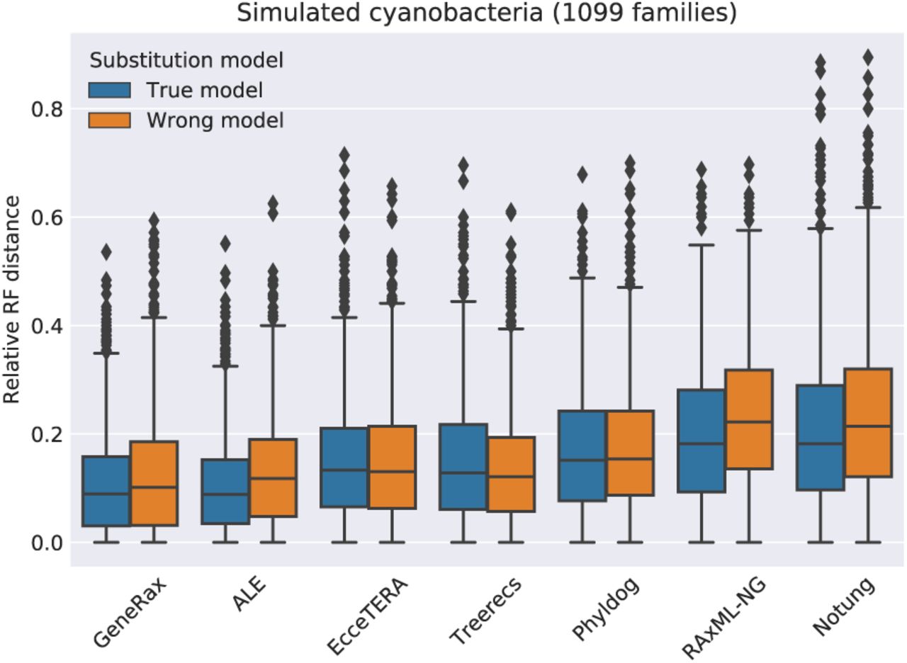
We show the relative RF distances between the 1099 simulated Cyanobacteria true trees and the respective inferred trees in Fig. 4. For methods that produce several gene trees per gene family (ALE and RAxML-NG), we average the distance over all the output trees.

Relative RF distances to true trees, by inferring gene trees with the true substitution model (LG+Γ+I) and a misspecified substitution model (WAG).
GeneRax and ALE perform better than all the other methods, except in the case of the misspecified substitution model where Treerecs also performs equally well. With the true model, STA methods that do not account for HGT but use a joint likelihood score (Phyldog and Treerecs) perform better than purely sequence-based method (RAxML-NG), but worse than methods accounting for HGT. Although EcceTERA accounts for transfers, it only performs as good as Treerecs, maybe because EcceTERA algorithm only uses parsimony. We hypothesize that Notung performs worse than all the other methods because it rearranges trees based on a parsimony score and an arbitrary support value threshold.
We show all results of the simulations where we vary parameters (DTL intensity parameters, etc.) in the Supplementary Material, and only include two representative plots here (FIG. 6). GeneRax finds the best trees under 90% of our simulation scenarios, but ALE finds almost as good trees on most of the simulations. Treerecs and Phyldog perform almost as well as GeneRax and ALE in the absence of HGT, but worse when the simulations contain HGT. Notung performs significantly worse than all SPA methods.

Branch score distance to true trees. We excluded from the plot methods with an average score above 4.

RF distance to true trees on simulated datasets. (a) Trees inferred with wrong species trees. All other parameters are fixed. (b) Trees inferred with varying DTL rates. We started from D = 0.1, T = 0.1 and L = 0.2, and multiplied all rates by a varying value (i.e. the ratio between the rates is constant).
Branch score distances to true trees
To compare the quality of the gene branch lengths, in terms of expected number of substitutions per site, we measured the average branch score distance (Kuhner and Felsenstein, 1994) between the inferred trees and the true trees (Fig. (5) with the phangorn R library (Schliep, 2010). GeneRax performs better than all competing tools. In particular, GeneRax has a significantly better average branch score distance (1.02) than ALE (1.48). A plausible explanation is that some of the competing tools do not optimize the branch lengths (ALE, EcceTERA, Notung), or not in terms of expected number of substitutions per site. When using those tools, users interested in branch lengths would need to add another tool to their pipeline (e.g., RAxML-NG).
Joint likelihood
We report the joint maximum likelihood scores of the gene trees obtained with the different tools in Fig. 7. As the true tree is generally not know for empirical data, and given that we are willing to accept the maximum likelihood criterion, we must assume that the trees yielding the best joint maximum likelihood is also the one that best explains the data. This approach of benchmarking ML tools on empirical datasets has been used repeatedly for assessing standard tree inference tools (Kozlov et al., 2019; Nguyen et al., 2015). The rationale for this is that standard tree searches based on the phylogenetic likelihood are inherently more difficult on empirical than on smooth and perfect simulated data. That is, differences between tree search algorithms might sometimes only be observable on empirical data. As expected, GeneRax finds the highest joint likelihood score. ALE is close to GeneRax, because it strives to optimize an approximation of the same model. As the remaining tools, implement distinct models, the comparison might appear as being unfair. However, we mainly regard this as a means of verifying that GeneRax can infer the best-known trees under its reconciliation model. Treerecs, Phyldog are also very close to GeneRax in absence of transfers, because they also a similar joint likelihood function. ALE is doing better than Treerecs and Phyldog in presence of HGT, because Treerecs and Phyldog only account for gene duplication and loss. RAxML-NG, EcceTERA and Notung do not rely upon any joint reconciliation likelihood model, which explains their low scores.
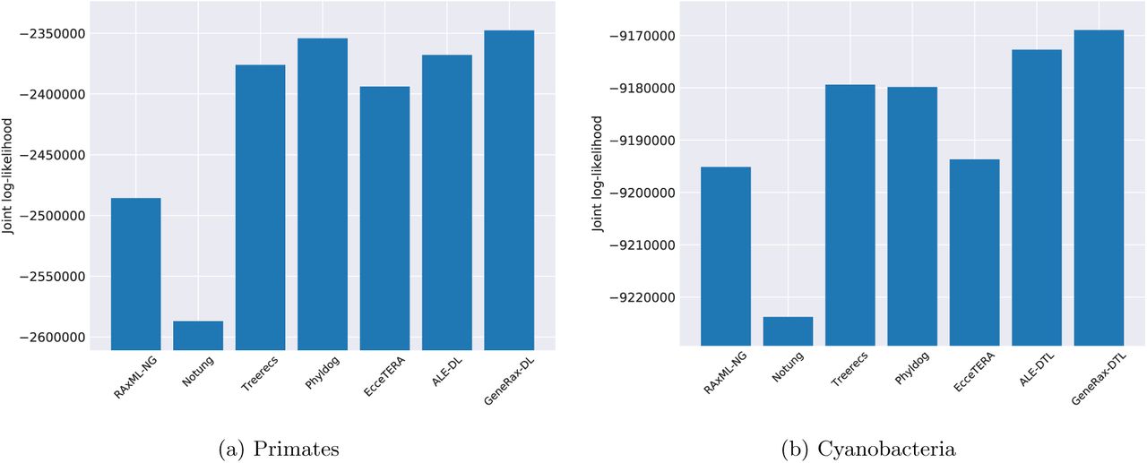
Log-likelihoods (the higher the better) evaluated with GeneRax. When evaluating the joint likelihood for Primates, we set the HGT rate to 0.
In addition, when running GeneRax on the empirical Cyanobacteria dataset, we recorded both, the reconciliation likelihood and the phylogenetic likelihood during the tree search (Fig. 8). We observer that the joint likelihood optimization occurs through an increase of the reconciliation likelihood at the expense of the phylogenetic likelihood. We made the same observation on all simulated and empirical datasets we experimented with. In general, we observed that our joint likelihood tree search heuristic is not efficient in improving the phylogenetic likelihood, and thus needs to start from trees with a high phylogenetic likelihood. For this reason, when the user does not provide a starting tree, we initially only optimize the phylogenetic likelihood, and subsequently start the joint likelihood optimization.

Reconciliation and sequence log-likelihoods during GeneRax tree search on the Cyanobacteria dataset. The sequence likelihood decreases while the reconciliation likelihood increases.
Sequential runtimes
We measured the sequential runtimes of all tools on the empirical Cyanobacteria dataset. Comparing runtimes is not straightforward: some tools are very fast, but require an external pre-processing step, as described in Table 2. For instance, Notung is the fastest tool, but it requires gene trees with support values as input, and obtaining those can be extremely time-consuming. For a fair comparison, we plot both the time spent in the gene tree inference tools alone, and the time spent in their respective pre-processing steps (Fig.9).

Sequential runtimes and additional overhead from precomputation steps (bootstrap trees with RAxML-NG for Notung and Treerecs, MCMC samples with MrBayes for ALE and EcceTERA, and RAxML-NG starting trees for GeneRax-raxml). The RAxML-NG column corresponds to the time spent in one single tree search. We represent times with a logarithmic scale.
When only considering the stand-alone runtimes of the tools, GeneRax is the slowest method. However, when including the pre-processing cost, GeneRax becomes the fastest STA approach. In addition, using only a single tool for the entire inference process substantially improves usability and reproducibility of the analysis.
Parallel efficiency
We measured the parallel runtimes of GeneRax for different numbers of cores. For this experiment, we ran GeneRax on the empirical Cyanobacteria dataset (1099 families), starting from RAxML-NG trees. We used 4 up to 512 cores. In Fig. 10 we plot the speedup as a function of the number of cores. Despite highly heterogeneous gene family MSA sizes (in terms of both number of sites and number of taxa, see Supplement Material), GeneRax achieves high parallel efficiency (0.7) on 512 cores.

Parallel speedup of GeneRax on the empirical Cyanobacteria dataset (1099 families), using from 4 to 512 cores.
We then measured the parallel efficiency of running the competing methods as described in the Experiments section, and present them in Fig. 11. GeneRax is the only tool that achieves good efficiency (0.7) because it parallelizes both, over, and within gene families, thereby achieving a ‘good’ load balance. Despite a similar two-level parallelization scheme, the parallel efficiency of RAxML-NG (scheduled with ParGenes, with one starting tree per family) is below 0.2. The reason for this is that ParGenes parallelizes individual tree searches over the sites whereas GeneRax parallelizes them over the SPR moves. Gene MSAs are often short, and there are typically not enough sites to allocate several cores per tree search with RAxML-NG. Other competing tools also fail to attain good parallel efficiency (<0.4), because they do not parallelize individual gene tree inferences, and are thus limited by the highest individual tree search runtime. GeneRax is less parallel-efficient when starting from random trees, because the initial phylogenetic likelihood optimization step is based on RAxML-NG code, which does not implement our two-level parallelization scheme yet.

Parallel efficiency of the different methods applied to the cyanobacteria empirical dataset on 512 CPU cores. We do not include pre-processing steps.
Discussion
An accurate, robust and fast approach
We present GeneRax, an open source STA gene tree inference software. GeneRax simultaneously accounts for substitution and DTL events. It performs a tree search to optimize a joint likelihood function, that is, product of the phylogenetic and the reconciliation likelihoods. It can handle multiple gene families in parallel. To the best of our knowledge, GeneRax is the first STA tool that does not require any pre-processing of the MSAs. Also, it does not require any arbitrary threshold settings or parsimony weights, and it can account for HGT.
On simulated datasets we demonstrate that GeneRax and ALE find trees that are closer to the true trees than those inferred by competing tools. We show that GeneRax is robust to inaccuracies in the assumed species tree and misspecified substitution models. Using two empirical datasets (Cyanobacteria and Primates), we confirm that GeneRax finds the best-scoring maximum likelihood trees among the tested tools, both, with, and without HGT. Finally, we show that GeneRax is not only faster than the tested competing methods (when accounting for the computational cost of the pre-processing steps), but also has a higher parallel efficiency, making it suitable for seamless large-scale analysis.
GeneRax is a production-level code. We kept its installation and its interface as simple as possible to facilitate usability. While most competing STA methods require input gene trees, sometimes, including additional information (e.g., support values), GeneRax can directly infer the gene trees from a set of given MSAs. This simplified analysis pipeline reduces the number of ad hoc choices users have to make: GeneRax does not require bootstrap-support thresholds, parsimony weights, MCMC convergence criteria, chain settings, proposal tuning, or priors. Reducing the number of arbitrary choices does not only yield the tool easier to run, but also substantially improves the reproducibility of the results. One could contest the parameters we used in our experiments for the pre-processing steps: Treerecs and Notung might not need 100 bootstrap trees to obtain reliable support values. ALE and EcceTERA might not need as many MrBayes runs, chains, or generations to correctly approximate the phylogenetic likelihood. In general, it is possible to run the pre-processing steps faster than in our experiments. When running the competing methods, we tried to use the parameters that favor result quality/confidence over short runtimes, as we would have done in a real analysis.
Future work
Despite the favorable evaluation results, GeneRax still faces several challenges.
First, the GeneRax reconciliation model does not take into account the branch lengths, neither in species tree, nor in the gene trees. This leads to information loss, and furthermore allows for transfers between non-contemporary species. We believe that further adapting and extending the reconciliation model could improve the quality of the results. For instance, one could exploit an ultrametric dated species tree and use speciation events to slice the species tree, as done in (Szöllősi et al., 2012b). However, slicing the species tree increases the number of inner species nodes quadratically, and thus incurs a substantial increase in computational cost.
Second, the GeneRax reconciliation model assumes that incomplete lineage sorting (ILS) does not occur. Some promising work (D Rasmussen and Kellis, 2012) has been conducted to combine gene loss, gene duplication, and ILS in a single model. We believe that a computationally efficient software that can account for ILS, DTL events, and substitutions in a probabilistic framework would represent a major breakthrough in phylogenetic inference.
Finally, GeneRax needs a known/given species tree to estimate the gene trees. To this end, we plan to extend GeneRax to co-estimate both, the gene trees, and the species tree, as done in (Boussau et al., 2012). An idea to solve this problem consists in inferring initial gene trees with non-STA methods, and then inferring an initial species tree that maximizes the reconciliation likelihood given these gene trees. Then in a second step, one can propose new species tree topologies, optimize the gene trees and DTL intensity parameters on this proposal, and update the species tree if the joint likelihood increases.
Acknowledgments
This work was financially supported by the Klaus Tschira Foundation and by DFG grant STA 860/4-2. G.J.Sz. received funding from the European Research Council under the European Unions Horizon 2020 research and innovation programme under grant agreement no. 714774 and the grant GINOP-2.3.2.-15-2016-00057. We thank Bastien Boussau, Eric Tannier, Celine Scornavacca and Wandrille Duchemin for discussions on the topic. We also thank Laurent Duret and Simon Penel for their valuable user feedback.
References


