

Abstract
Droplet-based scRNA-seq assays are known to produce a significant amount of background RNA counts, the hallmark of which is non-zero transcript counts in presumably empty droplets. The presence of background RNA can lead to systematic biases and batch effects in various downstream analyses such as differential expression and marker gene discovery. In this paper, we explore the phenomenology and mechanisms of background RNA generation in droplet-based scRNA-seq assays and present a deep generative model of background-contaminated counts mirroring those mechanisms. The model is used for learning the background RNA profile, distinguishing cell-containing droplets from empty ones, and retrieving background-free gene expression profiles. We implement the model along with a fast and scalable inference algorithm as the remove-background module in CellBender, an open-source scRNA-seq data processing software package. Finally, we present simulations and investigations of several scRNA-seq datasets to show that processing raw data using CellBender significantly boosts the magnitude and specificity of differential expression across different cell types.
1 Introduction
Droplet-based assays have enabled transcriptome-wide quantification of gene expression at the resolu-tion of single cells [1, 2]. In a typical scRNA-seq experiment, a suspension of cells is prepared and loaded into individual droplets. Poly(A)-tailed mRNAs in each droplet are uniquely barcoded and reverse-transcribed, followed by PCR amplification, library preparation, and ultimately sequencing. Quantifying gene expression in each cell is achieved by counting the reads from each gene that have a particular droplet barcode. The differential effects of PCR on different molecules can be reduced by using unique molecular identifier barcodes (UMIs), and counting the number of unique UMIs as a proxy for unique endogenous transcripts. This count information is then summarized in a count matrix, where counts of each gene are recorded for each cell barcode. The count matrix is the starting point of downstream analyses such as batch correction, clustering, and differential expression [3].
In an ideal scenario, a cell-free droplet is expected to be truly devoid of RNA molecules whereas a cell-containing droplet will yield transcripts originating only from the encapsulated cell. In reality, however, neither expectation is met. On the one hand, the cell suspension contains a low to moderate concentration of cell-free RNA molecules which leads to non-zero molecule counts even in cell-free droplets [4]. These cell-free RNA molecules, also referred to as ambient RNA molecules, have their origin in either ruptured cells or exogenous sources such as sample contamination. On the other hand, the shedding of capture oligos by beads in microfluidic channels as well as the formation of spurious chimeric molecules during the bulk mixed-template PCR amplification [5, 6] effectively lead to “swapping” of transcripts across droplets. The severity of these problems strongly depends on the tissue isolation protocol, the number of washing and size selection cycles, and PCR amplification conditioning and cycles [7].
The issue of background counts is particularly problematic in single-nuclei RNA sequencing experiments (snRNA-seq). The harsh nuclear isolation protocols produce a significant number of ruptured nuclei and a high concentration of cytoplasmic RNA in the suspension. In severe cases, the typical total UMI count distinction between droplets with and without nuclei nearly disappears and all droplets lie on a continuum of counts (e.g. see Fig. 1c). In such situations, successful downstream analysis hinges on our ability to (1) tell apart empty from non-empty droplets, and to (2) correctly recover the RNA counts from encapsulated cells or nuclei while removing background RNA counts.

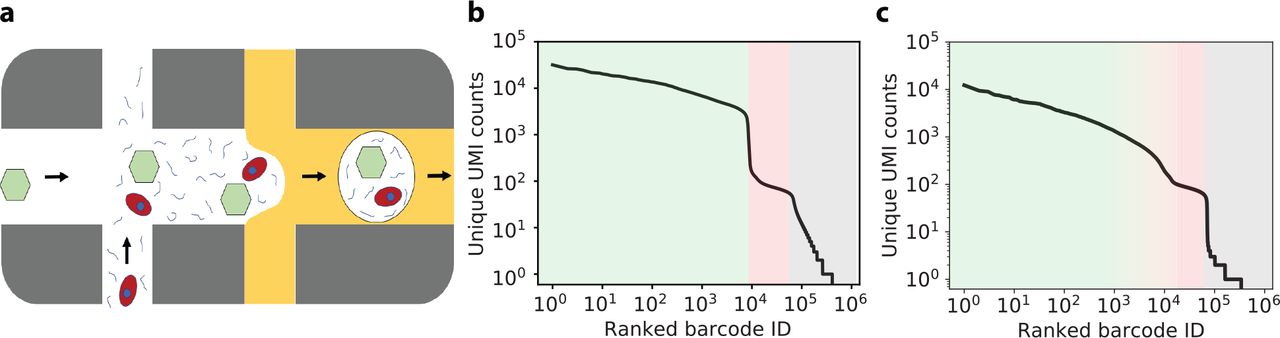
(a) Schematic diagram of the proposed source of ambient RNA background counts. Cell-free “ambient” RNAs (curved lines) are present in the cell-containing solution, and these RNAs are packaged up into the same droplet as a cell (red), or into an otherwise empty droplet that contains only a barcoded capture oligo bead (green hexagon). (b) Total unique UMI counts per droplet for the publicly available pbmc8k dataset from 10x Genomics (CellRanger 2.1.0). The x-axis denotes individual droplets sorted by total UMI count. There are approximately 8000 cells (pale green region). The “ambient plateau” is the region of the rank-ordered plot with ranked barcode ID greater than 8000 and less than about 80,000 (pale red region), where there are approximately 100 unique UMI counts per droplet. The tail of the plot contains barcodes with even fewer UMIs (pale gray region), which are putatively due to uncorrected barcode errors or impurity in capture oligo beads. (c) Same plot as panel (b), but for a dataset of rat heart nuclei (rat_6k). The transition between cells and the ambient plateau is much more ambiguous.
The presence of background counts can reduce both the magnitude and the specificity of differential gene expression estimates across different cell types. In cases where quantitative accuracy is important, for instance when searching for exclusive marker genes (such as during drug target discovery) or a small differential expression signal in a case / control setting, background counts can obscure or even completely mask the signal of interest. In some experiments, extremely high expression of a particular gene in one cell type can give rise to a large amount of background, making it seem as though all cells express the gene at a low level.
Here we introduce a deep generative model for inferring empty and cell-containing droplets, learning the background RNA profile, and retrieving uncontaminated counts from the non-empty droplets. Our proposed algorithm operates end-to-end starting from the raw counts, is fully unsupervised, and requires no assumptions or prior biological knowledge of either cell types or cell-type-specific gene expression profiles.
A major challenge in distinguishing background counts from biological counts for single droplets is the extreme sparsity of single observations, such that without a strong informative prior, the data obtained from a single droplet does not provide sufficient statistical power to allow inference of background contamination. Here, in analogy to nearest-neighbor pooling of similar observations, we utilize a neural network to learn the distribution of gene expressions across all droplets during the inference process. The learned distribution acts as a prior over background-corrected gene expression that effectively combines information from similar cells, allowing for significantly improved estimation of background contamination. Learning the prior distribution of biological counts and estimating the background contamination of individual droplets is performed simultaneously and self-consistently within an amortized variational inference framework.
We present extensive tests of our proposed method on both simulated and real datasets (whole-cell, single-nuclei, and mixed-species experiments). We show that:
Our method is superior to the currently existing methods in distinguishing empty and cell-containing droplets, in particular, in ambiguous regimes and challenging single-nuclei RNA-seq datasets (see Sec. 4.2, S.1, S.2 and Fig. 7, S1).
Our method successfully learns and subtracts background noise and artifactual counts from non-empty droplets and leads to significantly increased amplitude and specificity of differential gene expression (see Sec.Sec. 4.3, 4.4 and Fig. 8, 9, 10).
Our proposed method is presented as an easy-to-use command line tool. We utilize the Pyro probabilistic programming framework for Bayesian inference. GPU acceleration is necessary for fast operation of this tool. We refer to this method as remove-background, which constitutes the first computational module in CellBender, an open-source software package developed by the authors for preprocessing and quality control of scRNA-seq data. The current version of remove-background takes the output of 10x Genomics’ CellRanger v2 or v3 count pipeline as the input. CellBender modules are available on Terra [8], a secure open platform for collaborative omics analysis, and can be run on the cloud with zero setup.
This paper is organized as follows: we provide a more detailed account of the phenomenology of background RNA in Sec. 2. We present a probabilistic model for background-contaminated counts in Sec. 3 along with a brief overview of the inference algorithm and implementation in Sec. 3.2. We discuss the results on simulated and real data in Sec. 4. Further discussions and future extensions are discussed in Sec. 5.
2 The phenomenology of background RNA counts
In this section, we review the phenomenology of background RNA by examining three exhibits in different experiments. Next, we review a number of mechanisms that satisfactorily explain all aspects of the phenomenology. Some of these mechanisms have been noted by other authors, though we provide them in one place for completeness.
Exhibit 1
Examining the counts of total unique UMIs per droplet in a typical 10x scRNA-seq experiment reveals that there are thousands of high-count droplets followed by a much larger number of low-count droplets (See Fig. 1b-c and note the logarithmic scale of the axes). Here, the word “counts” is used as shorthand for counts of unique UMIs summed over all genes. The number of high-count droplets typically agree in order of magnitude with the expected number of cells given the protocol [2]. The low-count droplets typically have tens to hundreds of UMIs each (i.e. far fewer counts than high-count droplets), and significantly outnumber the expected number of cells. Therefore, these droplets are unlikely to have their counts originating from a physically encapsulated cell.
Exhibit 2
Experiments with mixtures of different cell types have shown that some of the transcripts in each droplet do not originate from the cell encapsulated within the droplet. That is, even for droplets that do contain cells, there is still some exogenous background noise in the count matrix.
Fig. 2 shows a scRNA-seq dataset generated using a mixture of human and mouse cells. It is noticed that for a few percent of the count data, human transcripts are assigned to a droplet where the vast majority of transcripts are mouse, and vice-versa. This mixing can happen when a human cell and a mouse cell are captured in the same droplet, but these “doublets” can be easily identified due to the fact that they have tens of thousands of counts from each species. Even droplets that do not contain doublets still have nonzero counts from transcripts of the other species (see the red inset of Fig. 2, for example). Droplets with tens of thousands of human counts typically have a few hundred mouse counts, and vice-versa.

A view of the public 10x Genomics human-mouse mixture dataset (hgmm-12k, CellRanger 2.1.0). Each dot denotes a droplet in the experiment. The y-axis shows the number of unique UMI counts of mouse genes in a given droplet, while the x-axis shows the number of unique UMI counts of human genes. Axes are plotted using a linear scale, with an inset zoomed in on mouse cells. The inset (red) shows that there are several hundred human gene counts in droplets that contain mouse cells.
Exhibit 3
The phenomenon of non-zero RNA counts in empty droplets is even seen in experiments where the preparation is entirely devoid of cells but rather contains a high concentration of spike-ins (e.g. see the publicly available ercc dataset from 10x Genomics [2, 9]). In this experiment, approximately 1000 droplets were prepared from the same spike-in soup and used for library production. Quite curiously, the total counts vs. sorted barcode plot looks similar to Fig. 1b: a first region including approximately 1000 high-count droplets, followed by thousands of droplets with approximately 100 UMIs each. The appearance of the second region resembling “empty droplets” is unexpected, since all droplets are filled uniformly with the same amount of spike-in transcripts.
We argue that the following mechanisms explain the entire phenomenology of background RNA in droplet-based scRNA-seq experiments:
Sequencing or synthesis errors in the droplet barcode
The presence of uncorrected sequencing errors in droplet barcodes or impurity of synthesized barcodes on capture beads will result in a spreading of transcripts across droplets. In particular, one expects a net flow of transcripts from RNA-rich (cell-containing) droplets to otherwise RNA-free (cell-free) droplets.
Quantitative estimates of barcode sequencing error indicate that far more empty droplets are observed than can be explained by sequencing error alone. The effective provisions for barcode error-correction employed by the 10x Genomics scRNA-seq protocol (using a whitelist, no homo-polymers, and a Hamming distance ≥ 2 between droplet barcodes) allows most barcode sequencing errors to be corrected. In our simulations using typical base substitution and insertion/deletion error rates, we found that at most 2 percent of erroneous droplet barcodes were corrected to the wrong barcode. Given that a typical 10x v2 scRNA-seq experiment yields less than 5 percent invalid barcodes, we estimate that at most 1 in 1000 transcripts would be mis-assigned due to wrong barcode error correction. This rate is 3 orders of magnitude lower than what is required to produce non-zero transcript counts in empty droplets as seen in typical experiments. The presence of error or impurity in barcode synthesis, however, might still explain part of the background RNA phenomenology. Unfortunately, details of the 10x barcode synthesis protocol are not public.
Presence of ambient RNA in the cell suspension
Cell-free “ambient” RNA that is physically present in the cell suspension and is encapsulated in a droplet will clearly contribute to the background while generating non-zero transcript counts in otherwise empty droplets. This mechanism is shown schematically in Fig. 1a. Cell-free RNA is present in the aqueous cell suspension, either as a result of normal biological processes or as a result of tissue dissociation, cell death, or other stresses experienced by cells during the isolation protocol which may cause cells to die or lyse. Such a mechanism has been proposed by others as well [1, 4, 10].
Barcode swapping and chimera formation
Swapping of droplet barcode between transcripts during mixed-template PCR amplification via formation of heteroduplex/chimeric molecules [5–7], and/or on the flowcell during sequencing [11], will spread transcripts across droplets and generate a background.
Chimeric fragments incorporate mRNA sequences from one original molecule and a droplet barcode (and UMI) either from a different original molecule or from a previously unused barcoded capture oligo. In the 10x Genomics protocol, there is a large amount of sequence complementarity, both in the Illumina primers as well as in the poly(T) region (the means by which these molecules were captured in the first place). As PCR progresses through many rounds, primers are depleted. Eventually, extension could be primed by (1) incomplete extension products from other molecules, as suggested by Dixit [6], or by (2) unused and inadequately washed capture oligos that were used to capture poly(A)-tailed mRNAs at the outset. These mechanisms would both result in transcripts which are assigned to the wrong droplets. This process of chimera formation is prone to occur in all mixed-template PCR reactions, and is not unique to scRNA-seq library preparation protocols [7].
Cross-contamination of capture oligo beads on the microfluidic device
The capture oligo gel beads (referred to as GEMs in the 10x Genomics scRNA-seq protocol) flow in a microfluidic channel (see Fig. 1a, green hexagons). The GEMs are tightly packed in the channel to achieve a precise flow control that allow their super-Poisson loading into droplets [2]. Since these gel beads are soluble in certain conditions in aqueous solution, it is reasonable to posit that some small number of capture oligos could be released from the GEM in the channel, leading to cross-contamination due to “ambient” capture oligos from other GEMs. Therefore, even if the GEMs were synthesized with high barcode purity to begin with, there could be some mixing in the microfluidic device. The downstream effect is similar to GEM impurity or barcode error, and produces a background. The appearance of thousands of low-count droplets in the spike-in experiment (cf. Exhibit 3 above) is likely to be associated with this mechanism.
We may summarize the above mechanisms in two main categories:
The mRNAs were physically present in the droplet at the time the droplet was formed. This is the “soup” or cell-free ambient RNA hypothesis. A small amount of cell-free ambient RNA was present in solution (due to cell death, lysis, etc.) at the time the droplets were formed, and some of this ambient RNA was packaged into each droplet, along with cells.
The mRNAs were not physically present in the droplet at the time the droplet was formed, but were later assigned to that droplet. This could happen in one of two ways: (1) a molecule’s droplet barcode was physically swapped to a cell-containing droplet barcode at some point in the protocol, (2) a molecule was mis-assigned to a different droplet barcode due to sequencing error or capture oligo impurity or contamination.
These two explanations could lead to different “background RNA” profiles. If cell-free ambient RNA was physically packaged into each droplet, then each droplet should contain a small sample of this same RNA profile, which could be related to cell expression or could be slightly different (for example, it could in principle incorporate an exogenous contaminant or a higher proportion of mitrochondrial mRNA if the source of cell-free RNA is related to cell death). If the cause of background RNA is instead barcode swapping, sequencing error, or capture oligo impurity, then it would be expected that the background RNA profile would be exactly the average of all the RNA sequenced in the experiment, because these mechanisms act at random.
3 A generative model for scRNA-seq data with background RNA
Here, we present an unsupervised end-to-end method for inferring empty and cell-containing droplets, learning the background RNA profile, and retrieving uncontaminated counts. This is achieved by modeling the data generation process from first principles based on the mechanisms of ambient RNA and chimera formation discussed earlier.
Since the background RNA counts are drawn from a fixed gene expression distribution, in principle, our many observations of empty droplets provide information that makes it possible to infer that distribution with high accuracy. However, in order to construct a complete generative model, we must also model the generation of true signal counts that come from cells. The challenging issue is our lack of a priori knowledge of the process that generates true biological transcript counts in a cell. Furthermore, we have several cell types in a typical experiment, and the fraction of transcripts present in cells that we measure at the end of the protocol is on the order of 10% or less (using 10x Genomics v2 or v3 chemistry, which generates at most tens of thousands of counts per cell). This phenomenon of measuring only a small fraction of what is present in the cell is sometimes referred to in the literature as “dropout”. This issue is further complicated by the presence of true biological variation such as bursting kinetics.
For these reasons, we would like our algorithm to be able to allow similar cells to share statistical power in order to learn the distribution of true biological gene expression. Grouping of cells into cell-type clusters in order to share statistical weight could be achieved in several ways, including a nearest-neighbors clustering or other graph-based diffusion methods. The methodology here employs a neural network as a flexible and trainable non-parametric distribution to act as a prior for biological gene expression (see NNχ in Fig. 3 and the forthcoming section for details).

Graphical model for RNA expression that combines ambient RNA and barcode swapping.
Here, the successful training of the neural module to represent the density of biological gene expressions relies on the validity of of the manifold embedding hypothesis, i.e. the possibility of mapping the true gene expression profiles of all cells in the experiment to a manifold of much lower dimensionality than the observable gene expression space. For example, an expression profile for a cell with 30,000 genes might be mapped to a lower-dimensional latent space of only 20 or 100 dimensions. This is a reasonable assumption provided that either the notion of “cell type” is roughly applicable, or otherwise, cells with continuous states (e.g. immature cells in a developmental trajectory, immune cells, etc.) can be described in terms of the activation of a low-cardinality set of co-regulated and co-functional gene modules. The current opinion in biology, as well as previous experiments with neural auto-encoders in the literature [12, 13], agree with the manifold embedding hypothesis.
Dimensionality reduction of scRNA-seq data using neural auto-encoders has appeared in other probabilistic models for the purpose of batch correction, visualization, and clustering [12–14]. In the context of our model, though, the neural network is utilized for learning the density of true biological gene expression. The learned density is then used as prior for sparse and background-corrected counts, and allows accurate estimation of background contamination fraction without additional regularization or resorting to heuristics.
We note that initially learned biological gene expression landscape may itself be contaminated with background RNA counts. However, as the inference procedure progresses and as the estimate of the background RNA profile improves, the maximum likelihood principle encourages the neural network to self-correct in a self-consistent fashion and learn to represent background-free gene expression profiles.
3.1 Model
The generative model for scRNA-seq count data that includes ambient RNA and barcode swapping is shown in Fig. 3. Throughout this section, we use n and g subscripts to refer to cell and gene indices on various vector and matrix random variables. zn ∈ ℝZ is the latent variable that encodes gene expression in a lower-dimensional space. χng is the fractional gene expression for each cell and lives on a (G − 1)-simplex in ℝG for each n, where G is the dimensionality of the full gene expression space. A decoder neural network (shown as the factor NNχ) parameterizes the mapping from zn to  is the fractional abundance of ambient RNA (on a simplex), and is a hyperparameter that we optimize over.
  is a cell-specific size factor.
  is a droplet-specific size factor for ambient counts. yn is a discrete binary random variable which is 1 if there is a cell in droplet n and 0 otherwise. ρn is the proportion of reads that are exogenous to droplet n. Finally, cng is the observed counts of gene g in cell n. The full model is as follows:

Here,  and
and  are all fixed hyperparameters that are derived automatically from the provided data. p is the prior probability that any given droplet contains a cell, and it is derived from the expected number of cells in the experiment. ϕα and ϕβ are general priors for the over-dispersion of the negative binomial count distribution1. ρα and ρβ are general priors for the contamination fraction ρn. The function NNχ(·) denotes a decoder neural network that maps the low-dimensional latent gene expression zn to the full gene expression χng on the (G − 1)-simplex. LogNormal distributions on the scale factors are justified by the empirical distributions of cell counts and empty droplet counts.
The specific negative binomial model used for observed counts, cng, requires elucidation. As mentioned earlier, the possible processes for background generation may be grouped into two categories: ambient RNA, and (effectively) random barcode swapping. The barcode swapping process results in a certain fraction of counts in each droplet, ρn ∈ [0, 1], that actually originated in other droplets. Because this process is equally likely to swap any two barcodes, the net effect is that the swapped molecules in any given droplet are effectively sampled from the average measured expression over the entire experiment (here denoted by  ). Ambient RNA molecules, on the other hand, may have a distinct composition as argued earlier and thus, are sampled from a different profile (denoted by
  ). Accordingly, we decompose the mean of the negative binomial in two main parts. The first part is the counts that physically originate in droplet
  , which includes a term for cell counts and a term for ambient RNA counts. The second part is the counts that did not physically originate in droplet n, but were erroneously assigned there later:
  . This expression is the product of three terms: the contamination fraction ρn, the term in parentheses that is proportional to the expected number of molecules physically encapsulated in the droplet, and finally the average gene expression profile,
  .
.
The model can be restricted to only ambient RNA by replacing the mean of the negative binomial with  . Similarly, the model can be restricted to only barcode swapping by replacing the mean of the negative binomial with
 . Results of these different models2 are compared in Section 4.
3.2 Inference
The probabilistic model described in the previous section entails several global (i.e. experiment-wide) and local (one for each cell) latent variables. Scalable approximate inference can be achieved using stochastic variational inference (SVI) [15] and amortization [16]. We provide a brief account of the inference strategy in this section.
The objective function to be optimized here is the evidence lower bound (ELBO):
 where X = {cng} is the observed data;
  is the bundle of tunable model hyperparameters, including the weights of the neural network NNχ (denoted by Wχ);
  is the bundle of latent variables; and q(Z | φ) is the variational ansatz shown in Fig. 4 and parameterized by
  . In the SVI methodology, one obtains argmaxθ,φ ELBO(X|θ, φ) via successive sub-sampling of data X and incremental updates of (θ, φ) using a stochastic optimizer. We refer the reader to Ref. 17 for a recent review.

Graphical model of the proposed amortized variational posterior.
The faithfulness of the approximate posterior to the true posterior is ultimately dependent on one’s choice of the variational ansatz, q(Z|φ). Fig. 4 shows the structure of our proposed ansatz. Generally speaking, we impose tunable parametric distributions over global latent variables while we infer local latent variables using auxiliary neural networks (often referred to as recognition networks). The latter technique is referred to as amortization and is the key to scalability of our algorithm to a theoretically unbounded number of data points (cells).
The posterior for zn is encoded by a neural network NNz which takes in observed counts cng and outputs (zn;μ, zn;σ); the latter parameterize the mean and scale of an assumed Gaussian posterior distribution for zn:

Note that this encoder network for zn, together with the decoder network that maps zn to χng, form the auto-encoder structure mentioned earlier.
The posterior for  , the scale-factor for biologial counts, is likewise encoded by a neural network NNd which takes in cng and outputs
  , a strictly-positive scale-factor per droplet. Additionally, we allow
  to be a tunable parameter to characterize the spread in sizes of cells. We pose the following ansatz for the posterior of
  :
:

In practice, we found it beneficial to further provide a hand-crafted feature, log(∑gcng) (logarithmic total UMI count) to NNd. Intuitively, this feature gives a strong signal for inferring the “size” of the encapsulated cell along with the droplet-specific transcript capture efficiency.
The posterior for yn is encoded by a neural network NNy which takes in cng and  and outputs qn, the posterior Bernoulli parameter:

Again, we found it beneficial to provide log(∑gcng), as well as  (i.e. the naïve background-corrected counts), as hand-crafted features to NNy.
3.2.1 Technical Remarks
The default architecture of the auto-encoder for zn has one hidden layer of 500 units, and the encoded dimension of zn is 20. The encoder for  defaults to three hidden layers of size (5, 2, 2), while the encoder for yn defaults to two hidden layers of size (100, 10). Softplus non-linearities are used throughout. In practice, the algorithm is not very sensitive to the architecture of NNy and NNd, but the dimension of the latent zn does influence the results. In general, a larger latent dimension (up to 200) encourages a more faithful reconstruction of the data with less imputation. A smaller latent dimension encourages imputation and the sharing of gene expression information across similar cells.3
For numerical stability and to preclude vanishing gradients, the actual implementation handles probabilities in logit-space. During training, the log probability of zn is only computed for droplets which have been found to contain cells (that is, for droplets n where a sample from yn is 1). The discrete latent variable yn cannot be re-parameterized, and so we use complete enumeration over cell / no cell (yn being 1 or 0) in our variational posterior to reduce variance. Integration over the continuous latent variables appearing in the ELBO is done using a single Monte-Carlo sample as usual.
Training happens in random mini-batches. Each full epoch trains on a fixed subset of barcodes from the dataset as well as a randomly-sampled subset of empty droplet barcodes that changes each epoch (this is done in order to cover the tens of thousands of empty droplets without taking excessive computation time)4.
The training loop converges typically within 100 to 300 epochs. For a typical 10x scRNA-seq experiment containing 5-10 thousand cells, the total runtime of the tool ranges between 30 minutes to several hours using an NVIDIA Tesla K80 GPU, depending on the size of the dataset and chosen parameters.
3.3 Implementation and Usage
We have implemented the model and the inference method using the Pyro probabilistic programming language [18] and PyTorch [19] and presented it as a user-friendly and stand-alone command line tool. We refer to this tool as remove-background which consti tutes the first computational module in CellBender, an open-source software package developed by the authors for pre-processing and quality control of scRNA-seq data.
CellBender can be obtained from https://github.com/broadinstitute/CellBender. Additional documentation is available at https://CellBender.readthedocs.io. CellBender modules are also available on Terra [8], a secure open platform for collaborative omics analysis, and can be run on the cloud with zero setup.
3.3.1 remove-background inputs
The current version of remove-background takes the raw HDF5 file from 10x Genomics’ CellRanger v2 or v3 count pipeline as the input. Support for additional scRNA-seq protocols (e.g. drop-seq) will be added in the future.
3.3.2 remove-background outputs
The output of CellBender remove background provides several useful quantities: (1) inferred background-subtracted count matrix, (2) probability that each droplet contains a cell, and (3) low-dimensional latent representation of gene expression for each cell. The background-subtracted count matrix is defined as:
 where
where  and
and 
 . Here
  and zn;μ are obtained from the learned encoder networks NNd and NNz, respectively. The probability that each droplet contains a cell is given by qn, the latent variable encoded by NNy. The low-dimensional latent representation of gene expression is given by the encoded zn;μ for each cell.
Note that  is the approximate MAP estimate of the negative binomial mean rate parameter μ, as obtained by replacing ρn → 0 and
  . In other words, it is the gene expression rate in the absence of barcode swapping and ambient RNA. Importantly, this quantity is not quantized and the entries of
  contain a large number of non-zero yet very small numbers. In order to produce a sparse count matrix, we quantize
  as follows: each nonzero entry in
  is truncated to an integer and rounded up with probability equal to its decimal value (i.e. 1.2 is rounded up to 2 with probability 0.2).
4 Results
Here we examine a few datasets in order to demonstrate the outputs of remove-background and to assess its performance on real data. To validate the inference procedure, we first examine a simulated dataset. Next we take a look at cell calling and background removal in a real dataset where we have some knowledge of the truth. Finally, we process a real dataset with remove-background in order to explore the downstream effects on a standard differential expression analysis.
4.1 Consistency check on simulated data
As a check on the inference procedure, we have run several experiments on simulated data. Datasets were generated based on expression profiles pulled from real public 10x Genomics datasets. Fig. 5 shows the results of inference using a simulated dataset with 30,000 genes, generated according to the ambient RNA model. The simulated data has 3 “cell types” with unique underlying expression profiles. While the expression profiles are different from one another, they mimic cell clusters in real datasets. This results in expression profiles that are very similar for most genes. Two of the cell types have between 400 and 500 cells, while the third type has only 50 cells. Ambient expression in the simulation is a weighted average of total expression.

Results of inference on a simulated dataset with three cell types. (a) PCA visualization of the learned latent gene expression (20 dimensions) shows three clusters that correctly separate the cell types. (b) Matrix showing cosine distance between the true and learned expression profiles for ambient RNA as well as cell expression. (c) Same data as in (b), but plotted as a matrix of scatter plots. Each point on each scatter plot is one gene. Axes are normalized expression in log-space.
Fig. 5 demonstrates that the latent variable model is able to learn a decent prior on the true expression profile of cells, and that the inferred background-removed expression very closely matches the truth.
4.2 Accurate detection of empty droplets
The posterior probability qn that droplet n contains a cell is a direct result of the inference procedure. While this determination can be trivial in some pristine datasets, complicated experimental factors often make determination challenging in real datasets. A variety of heuristics are typically employed in order determine cutoffs for thresholding cells versus empty droplets. More principled approaches have recently been developed, including EmptyDrops [10], which uses statistical tests to ascertain which droplets have expression profiles significantly different from empty droplets, and DropEst [20], which distinguishes empty and non-empty droplets using a linear classifier trained on features extracted from a set of a priori known empty and non-empty droplets.
These approaches, however, depend on having prior knowledge of a range of cell-free droplets (e.g. being able to discern the empty droplet region in the ranked barcode plot; see Fig. 1b). As mentioned in the introductory remarks, this requirement is not always met in heavily contaminated datasets where background RNA counts are similar in magnitude to RNA cell counts. In our proposed algorithm, the determination of empty vs. non-empty droplet is a byproduct of inference in the context of our latent variable model, which in principle can learn to disentangle background RNA counts from cell RNA counts. As such, while our approach benefits from a decent initialization from a range of potentially empty droplets, it is not a necessity.
Fig. 6a shows the posterior cell probabilities for the first 22,000 droplets of the public 10x Genomics hgmm-12k human-mouse mixture dataset (v2 chemistry, CellRanger 2.1.0). Note that the algorithm in general identifies cells and empty droplets as expected, and that the transition between the two is not based on a hard UMI cutoff. Further exploration of the gene expression profiles of these called cells is shown in the supplement, Fig. S1. A determination of cell / no cell can be obtained by thresholding based on the posterior probability, qn. The algorithm converges to largely binary probability values, so the precise choice of threshold value hardly makes a difference in practice.
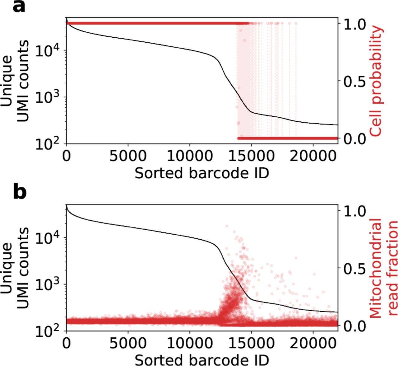
Result of inference on the 10x Genomics human-mouse mixture dataset hgmm-12k. (a) Two plots are overlaid. The black line is the UMI counts per droplet (barcode), while the red dots with dashed lines are the probabilities that each droplet contains a cell. (b) Fraction of unique UMI counts from mitochondrial genes. The transition region between cells and empty droplets has a high fraction of counts from mitochondrial genes.
As suggested by previous authors [10, 20], other criteria can be used to post-filter cells, including mitochondrial read fraction. Fig. 6b is a plot of the fraction of reads per droplet that come from mitochondrial genes. It can be clearly seen that many cells in the transition region exhibit a high fraction of mitochondrial genes (possibly dead or dying cells), and because they are distinct from empty droplets, they are determined to have a high probability of containing cells. After filtering cells based on mitochondrial gene count, some of these lowest-count cells will be filtered out. This is the recommended workflow.
Figure 7 shows cell calling on a more challenging dataset. The dataset corresponds to a single-nuclei extraction experiment. As mentioned in the introductory remarks, the harsh nuclear isolation protocols produce a significant number of ruptured nuclei and a high concentration of cytoplasmic RNA in the suspension. The rank-ordered total UMI plot of this dataset is shown in Fig. 1c.

Comparing CellBender remove-background cell calling with several existing methods on a challenging single-nuclei RNA-seq dataset rat_6k. (a) Four panels showing the same UMI curve where cells are called using four different algorithms: CellRanger 2.1.1 (5000 expected cells), CellRanger 3.0.2 (5000 expected cells), EmptyDrops (lower UMI count threshold = 100, Bonferroni-corrected FDR < 1%), and CellBender remove-background (5000 expected cells). (b) A standard analysis of the dataset using scanpy. Cell clusters are visualized using UMAP in the upper left panel. The three other panels show cells in blue that were called by CellBender remove-background but excluded by another algorithm. See Table S1 for a quantitative comparison.
We compare the cell calls made by CellBender remove-background with three other methods in common use: CellRanger v2, CellRanger v3, and EmptyDrops. Panel (a) shows that CellBender remove-background generally calls more cells compared to CellRanger, many of which lie further down the UMI curve. The set of cells called by CellBender remove-background contains all the cells called by CellRanger v2, v3, and EmptyDrops after the typical filtering by gene complexity and mitochondrial fraction. Panel (b) shows that the extra cells called by CellBender remove-background do in fact cluster together with cells called by the other algorithms, suggesting that they are legitimate cell calls and are not empty droplets.
EmptyDrops, when run with the default parameters (lower UMI threshold set to 100, Bonferroni-corrected FDR < 1%), calls many low-UMI-count cells that CellRanger v2 and v3 miss, though, it also curiously misses a large number of relatively high-UMI-count droplets along the rank-ordered UMI plot. We notice that the most populous clusters are also the most enriched in cell calls missed by EmptyDrops (Clusters 0, 1, 2; see Table S1).
We hypothesize that the issue originates from the frequentist approach used in EmptyDrops. Since the background profile indeed resembles the gene expression profile of the most abundant and transcript-rich cell types, the expression profiles of these cells are accidentally compatible with the background. Therefore, the Dirichlet-Multinomial p-values obtained on a single-droplet basis may not reach statistical significance for droplets that contain one of the major cell types, in particular, if the background pseudo-count scale α (a model parameter in EmptyDrops) is determined to be too large. By default, EmptyDrops determines α via a maximum likelihood procedure. We found that overriding α manually and using a smaller value generates more statistically significant cell calls, as expected. Checking the soundness of these extra cell calls is beyond the scope of this work.
We remark that CellBender remove-background does not suffer from this caveat since it effectively performs Bayesian model comparison using informative priors for both hypotheses (empty model yn = 0, non-empty model yn = 1; see Eq. 1). The expression profile and the expected UMI count of the abundant cell types (and the background) are initially learned from the low- and high-count droplets, this prior information is used in comparing the two models, and the priors and posteriors are updated until a self-consistent solution is achieved. Further analysis and discussions are provided in supplementary Section S.2.
4.3 Decreased magnitude of cross-species transcripts in barnyard experiments
A useful benchmark dataset for removal of background RNA is a mixed-species (“barnyard”) dataset, where two cell lines from different species are combined and run through the experiment together. This would ideally result in droplets containing exclusively counts from one genome or the other, but due to the presence of background RNA, this is not the case. Here we use the public 10x Genomics human-mouse mixture dataset hgmm-12k. The raw UMI counts per droplet were shown earlier in Fig. 2.
The output of CellBender remove-background is shown in Figure 8. Ideally, what we would expect is that human counts are removed from the mouse cell population, and that mouse counts are removed from the human cell population. This is in fact what we observe, as shown using different models in orange, green, and red. The different models are those described in Sec. 3. By default, remove-background runs the full model, shown as the red data points.

The result of processing the hgmm-12k 10x Genomics public dataset using CellBender remove-background. Each dot is a droplet in the experiment. Blue is the raw data, while the other colors are the results of background removal. The y-axis shows the number of unique UMI counts of mouse genes in a given droplet, while the x-axis shows the number of unique UMI counts of human genes. (a) Magnified x-axis, showing removal of human genes from mouse cells. (b) Magnified y-axis, showing removal of mouse genes from human cells.
The number of cross-species background counts is reduced by more than an order of magnitude, from a few hundred per droplet to tens of counts or fewer per droplet. It is worth re-emphasizing that this is a completely unsupervised approach, and that the algorithm does not know anything about human genes or mouse genes, or that this is a mixture experiment.
4.4 Increased specificity of differential expression
To demonstrate the effect of background RNA removal on downstream analyses, a standard analysis workflow was carried out on the public 10x Genomics pbmc8k dataset (v2 chemistry, CellRanger 2.1.0) using Seurat v3 [3]. The results of the exact same analysis, with and without remove-background preprocessing, are shown in Fig. 9.

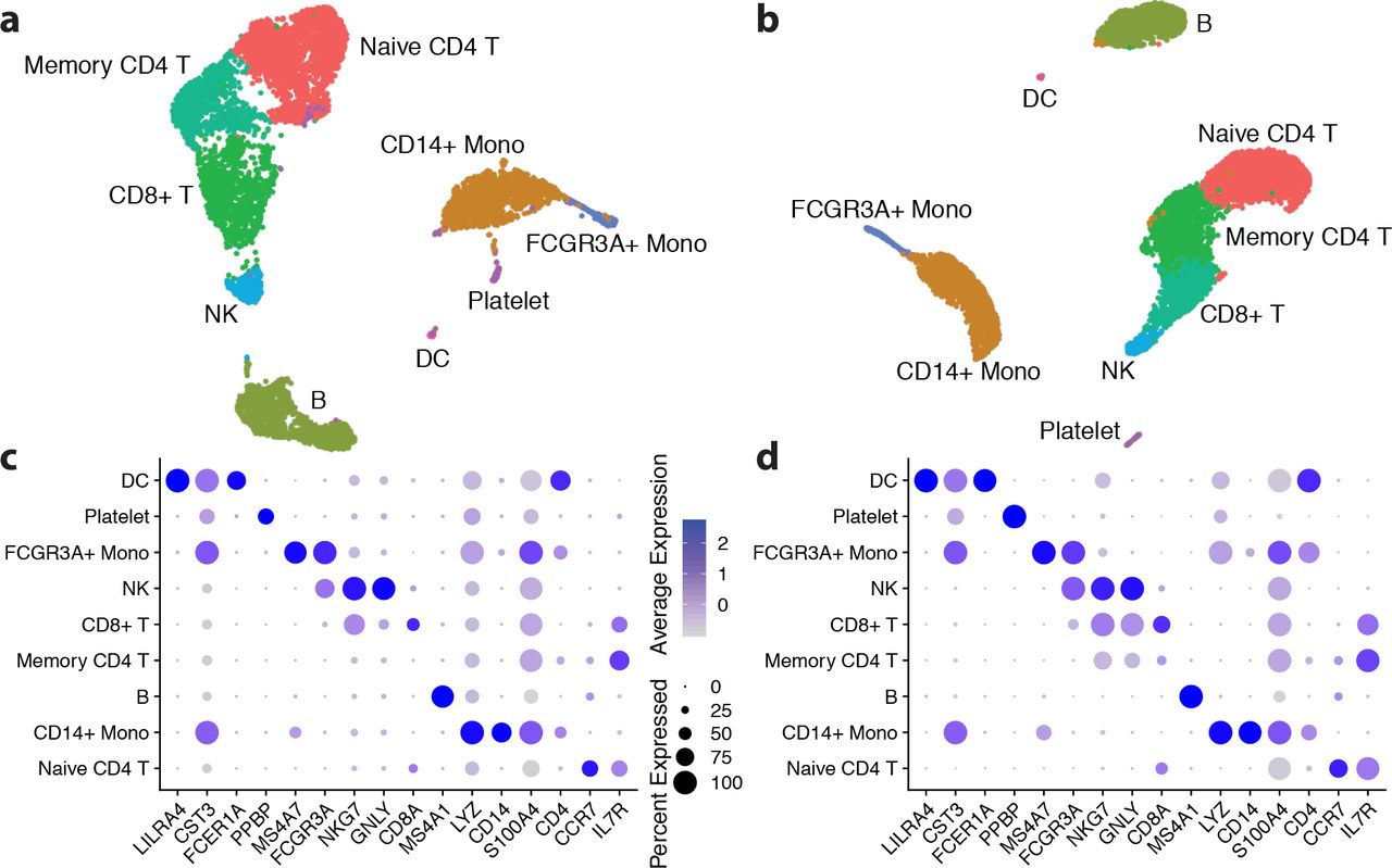
Analyses in Seurat using the publicly-available 10x Genomics dataset pbmc8k, CellRanger UMAP visualizations of (a) the original dataset and (b) the dataset processed with CellBender remove-background. The same clusters were obtained using the same value for Seurat’s FindClusters resolution parameter (0.18). The dot plots display a standard visualization of pre-defined marker genes for these cell types for (c) the original dataset and (d) the dataset processed with CellBender remove-background.
Cells were determined using qn > 0.9, and these cells were used in both analyses. Cells were further filtered using cutoffs for number of nonzero genes, percent mitochondrial reads, and an upper limit for UMI counts. The resolution parameter of Seurat’s FindClusters method was chosen so that the raw data and the remove-background pre-processed data would exhibit the same number of clusters. Notably, the same cell clusters can be recovered using the exact same Seurat analysis, and there is less background RNA obscuring the differential expression signal. In panel (d), the genes CST3 and LYZ in particular have noticeably reduced expression in several clusters, as compared to panel (c). Fig. 10 shows the effect on LYZ expression across clusters in more detail.

Same analysis as in Fig 9, here showing violin plots of the expression of the gene LYZ in each cell cluster. y-axes are unique UMI counts per cell. Background counts of LYZ decrease between (a) the original data, and (b) the data pre-processed with CellBender remove-background. This improves the differential expression signal.
Table 1 shows the differential expression for LYZ and CST3 between CD14+ monocytes (where expression is expected) and B cells (where expression is not expected), calculated in Seurat as the average log fold change by FindMarkers (using the bimod likelihood ratio test). The differential expression increases substantially after subtracting background RNA.
Differential expression effect size (log fold change) between “CD14+ Monocytes” and “B cells”
Finally, the low-dimensional latent representation of true gene expression inferred by remove-background, zn, is also interesting to examine. UMAP [21] is used to project the 200-dimensional latent space into a 2-dimensional view in Figure 11a. All the expected cell types show up as clusters in the latent space. An additional cluster shows up in between several of the other large clusters (colored purple), which may correspond to doublets. The UMI counts per cluster, shown in Fig. 11b, seem consistent with the hypothesis that the purple cluster may in fact be doublets, as does the gene expression profile of the cluster in Fig. 11c. This cluster formation in the latent space is quite robust to the choice of the number of latent dimensions as well as to downsampling of the dataset.
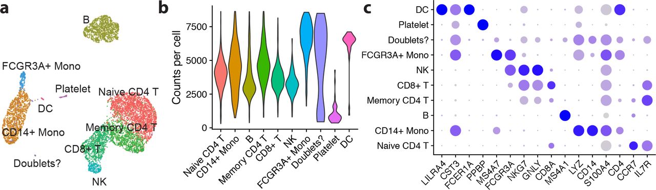
Analysis of the 10x Genomics pbmc8k dataset using Seurat, but using the inferred latent representation for gene expression, zn, instead of the typical normalization, variable gene selection, and PCA workflow. (a) Latent gene expression projected into two dimensions using UMAP (arbitrary scale). The clusters that naturally form in latent space can be seen to correspond to real cell types. (b) The UMI counts per cell for each cluster, where purple is a possible doublet cluster. (c) Dot plot showing gene expression of pre-defined marker genes. Putative doublet cluster has a mix of gene expression.
5 Discussion
The CellBender remove-background tool is presented here as a method for removing background noise from droplet-based scRNA-seq count matrices. remove-background can be used as a pre-processing step in any scRNA-seq analysis pipeline and is especially helpful for datasets with a lot of ambient RNA or barcode swapping. Ambient RNA can be an issue for snRNA-seq data in particular, due to the difficult nature of nuclear isolation protocols.
To the best of our knowledge, CellBender remove-background is the first unsupervised method for modeling and removing background RNA counts from scRNA-seq datasets. There has been previous work addressing the removal of background RNA, including SoupX [4] for removal of ambient RNA, and methods for attenuating background counts due to chimeric molecules [6]. In practice, the operation of SoupX is largely manual and relies on the user’s prior knowledge of cell-type-specific gene expression, as well as providing a list of genes for estimating background RNA fraction in cells. The method introduced in Ref. 6, while being effective at reducing the number of chimeric molecules, does not include provisions for the removal of physically encapsulated ambient transcripts.
S Supplementary Material
S.1 Cell calling in the difficult transition region
remove-background performs probabilistic cell calling, i.e. determining which droplets are empty and which are not. The decision about cell / no cell is made on the basis of both UMI counts and the gene expression profile. In the full model (Eqn. 1), the total observed RNA count is drawn from a negative binomial distribution whose mean includes a term for cell expression, if a cell is present, and an ever-present contribution from ambient RNA and random barcode swaps. The size of the background contribution must be consistent with the measured ambient RNA plateau in empty droplets. Additionally, the ambient RNA is drawn from an ambient RNA profile that is a global value for the whole dataset. If the gene expression in a droplet differs significantly from the ambient RNA profile, even if the total UMI counts are similar, this difference will be the basis for determining that a droplet is not ambient background alone.
The most difficult cells to call are those in the “transition” region in the rank-ordered total UMI plot. Cell calls for the 10x Genomics hgmm-12k dataset are shown in Fig. S1. Panel (a) shows which droplets were determined to have cells. The difficult transition region, where the calls are not obvious, are labelled “ambiguous”. Cell calls from this region are shown in green, while empty droplets are shown in red. The “ambiguous” region was found to consist of 451 cells and 4329 empty droplets. Fig. S1b shows the normalized gene expression profiles of different groups of droplets as scatter plots against one another. The lower left panel shows that cells called in the ambiguous region have gene expression that largely correlates with that of obvious cells. Likewise, the upper right panel shows that those droplets from the ambiguous region that were determined to be empty have expression profiles that match the profile of obviously empty droplets. Finally, plotting the expression of ambiguous empty droplets vs. obvious cells (upper left panel) and ambiguous cells vs. obvious empty droplets (lower right panel) shows a significantly weaker correlation.
This example demonstrates that as expected, remove-background utilizes both the total UMI count as well as the observed gene expression in cell-calling.

Determination of cells versus empty droplets in the hgmm-12k public dataset from 10x Genomics (v2 chemistry, CellRanger 2.1.0). (a) Cells called by remove-background. “Ambiguous” here refers to difficult-to-call droplets in the transition region. Each droplet has been labelled cell or empty. (b) Normalized gene expression profiles from the droplets shown in (a). Expression is summed over 400 droplets in the case of cells, or 4000 droplets in the case of empties. Each dot on each scatter plot is one gene. Human genes are in blue; mouse genes in red. Note that remove-background correctly calls cell-containing and empty droplets with very similar UMI counts in the transition region on the basis of gene expression.
S.2 Cell calling for a dataset of single-nuclei extraction
We run CellBender remove-background, CellRanger v2.1.1, CellRanger v3.0.2, and EmptyDrops (as in Bioconductor v3.9) with the default arguments on the dataset (see the caption of Fig. 7 for details). We removed all droplets outside of the union of cell calls made by the four methods. Next, we ran a standard scanpy analysis to cluster the cells and to find marker genes. Cells with mitochondrial read fraction greater than 1% (after CellBender remove-background correction) have been removed, as well as cells with fewer than 200 unique genes expressed at nonzero levels. Cells with unusually high numbers of unique genes expressed at nonzero levels, as well as with unusually high UMI counts, are also eliminated. The cutoff for “unusually high” is the 75th percentile of the distribution, plus the inter-quartile range. These filters are commonly employed to remove outliers and doublets from the analysis.
Figure S2 shows a UMAP plot displaying the clusters (same data as in Figure 7b) on the left. All cells are in gray, and the cell calls unique to CellBender remove-background are highlighted in blue. Also shown is a dotplot containing the marker genes for each cluster on the right. Table S1 shows the number of cells called by the four methods aggregated per cluster.
We notice that (1) CellBender remove-background calls more cells than CellRanger or EmptyDrops, and (2) CellBender remove-background does not miss any of the cells called by the other methods. We argue below that (1) the extra calls made by CellBender remove-background are valid, and (2) excluding these cells implies discarding a significant, and biased, slice of the dataset.
On the one hand, we notice that the extra cell calls made by CellBender remove-background are distributed essentially uniformly across the eight clusters. Crucially, the extra cell calls do not form a cluster of their own: had these extra cells been actually empty droplets, we would expect their expression profile to regress toward the background profile and cluster together. Even for clusters enriched with extra calls by CellBender remove-background (e.g. cluster 3), we find very specific marker genes. Again, this would not be expected if CellBender remove-background were erroneously identifying empty droplets (which would not be marked by unique marker genes that are absent from the other cell clusters).
On the other hand, we notice that the other methods, in particular EmptyDrops, fail to call a large fraction of cells in the most populous clusters. For instance, EmptyDrops has detected 8 cells in Cluster 2 (after quality-controlling cells as described above), compared to 861 cells called by CellBender remove-background (see Table S 1). This cluster, which can be identified as cardiomyocytes, is populous while also producing disproportionately more transcripts per nucleus. This implies that the ambient background profile is likely to closely resemble that of cardiomyocytes. As such, the Dirichlet-Multinomial likelihood model employed in EmptyDrops does not yield a statistically significant probability of being non-empty for cardiomyocyte-containing droplets. In contrast, CellBender remove-background learns the expression profile of cardiomyoctyes from high-count droplets and is not impacted by this phenomenon.
Cells called by various methods for rat_6k single-nuclei RNA-seq dataset.

Clusters identified using a standard scanpy analysis using the Louvain clustering algorithm with resolution parameter 1.0. Blue marks cells called only by CellBender remove-background. Marker genes for each cluster (Wilcoxon rank-sum test) are displayed in a dot plot. This plot demonstrates that even for cluster 3, which has a high number of cells called only by CellBender remove-background, there are identifiable marker genes that are largely cluster-specific. These extra cells are not background.
Acknowledgements
The authors thank Luca D’Alessio, Mark Chaffin, Alessandro Arduini, Amer-Denis Akkad, NathanTucker, Patrick Ellinor, Yossi Farjoun, Timothy Tickle, and Ambrose Carr for insightful discussions at various stages of this project. SF and MB acknowledge financial support from Broad-Bayer Precision Cardiology Lab (PCL). MB acknowledges additional support from the SPARC Grant Development of Production-Grade Computational Methods for Single-Cell Genomics from the Broad Institute. The unpublished rat_6k single-nuclei RNA-seq dataset was generously contributed by the PCL.
Footnotes
↵1 In our parameterization of the negative binomial distribution NegativeBinomial(μ, Φ), μ denotes the mean and Φ parameterizes the variance as μ + Φ μ2.
↵2 The default mode for remove-background uses the full model as specified in Eq. (1), but the user can specify the ambient-only or swapping-only model via command line arguments.
↵3 The sizes of the neural network decoder and encoders can be specified using command line arguments. In our experiments, we found imputation to be minimized or fully eliminated using a high-capacity neural network, e.g. by setting --z-dim 200 --z-layers 1000.
↵4 The fraction of each minibatch that is composed of these randomly-sampled empty droplets can be specified using a command line argument.
References


