

Abstract
Two endemic sardines in Lake Tanganyika, Limnothrissa miodon and Stolothrissa tanganicae, are important components of the lake’s total annual fishery harvest. These two species along with four endemic Lates species represent the dominant species in Lake Tanganyika’s pelagic fish community, in contrast to the complex pelagic communities in nearby Lake Malawi and Victoria. We use reduced representation genomic sequencing methods to gain a better understanding of possible genetic structure among and within populations of Lake Tanganyika’s sardines. Samples were collected along the Tanzanian, Congolese, and Zambian shores, as well as from nearby Lake Kivu, where Limnothrissa was introduced in 1959. Our results reveal unexpected cryptic differentiation within both Stolothrissa and Limnothrissa. We resolve this genetic structure to be due to the presence of large sex-specific regions in the genomes of both species, but involving different polymorphic sites in each species. Additionally, we find a large segregating inversion in Limnothrissa. We find all inversion karyotypes throughout the lake, but the frequencies vary along a north-south gradient within Lake Tanganyika, and differ substantially in the introduced Lake Kivu population. Little to no spatial genetic structure exists outside the inversion, even over the hundreds of kilometres covered by our sampling. These genetic analyses show that Lake Tanganyika’s sardines have dynamically evolving genomes, and the analyses here represent a key first step in understanding the genetic structure of the Lake Tanganyika pelagic sardines.
Introduction
Identifying the genetic basis of ecological adaptation is a high priority in evolutionary biology and has important implications for population management. Recent research in this field focuses on genomic regions with reduced recombination rates, such as chromosomal inversions (e.g. Berg et al. 2017; Christmas et al. 2018; Kirubakaran et al. 2016; Lindtke et al. 2017), sex chromosome regions (Presgraves 2008; Qvarnstrom & Bailey 2009) or both (Connallon et al. 2018; Hooper et al. 2019; Natri et al. 2019). The reduced recombination rates in such chromosomal regions enable local adaptation even when gene flow is high (Kirkpatrick & Barton 2006). Furthermore, it appears that these mechanisms for restricted recombination are more prevalent in sympatric than in allopatric species, and fixation of inversions is faster in lineages with high rates of dispersal and gene flow (Berg et al. 2017). These patterns are consistent with theory in which the presence of gene flow favours diversification of chromosomal rearrangements caused by locally adapted loci (Berg et al. 2017; Kirkpatrick & Barton 2006).
Pelagic habitats represent uniform environments that allow for high dispersal rates due to the lack of physical barriers. Well known examples of species from pelagic habitats that carry chromosomal inversions or sex loci include Atlantic cod (Cadus moruha) (Berg et al. 2017; Kirubakaran et al. 2016), Atlantic herring (Clupea harengus) (Lamichhaney et al. 2017; Martinez Barrio et al. 2016) and stickleback (Gasterosteus aculeatus) (Jones et al. 2012). In Atlantic cod and herring populations, low genome-wide divergence is interspersed with highly divergent inverted regions. These inversions in cod distinguish between resident and migrating ecotypes (Berg et al. 2017; Kirubakaran et al. 2016), and in herring they separate spring and fall spawners (Lamichhaney et al. 2017; Martinez Barrio et al. 2016). Additionally, inverted genomic regions in sticklebacks are involved in the divergence between lake and stream ecotypes (Marques et al. 2016; Roesti et al. 2015).
From management perspectives, pelagic mixed stocks are notoriously difficult (Belgrano & Fowler 2011; Botsford et al. 1997) and part of this challenge lies in identifying Management Units (MUs) which are demographically independent and genetically distinct populations. In a uniform habitat without physical barriers, low genetic differentiation is typical, as there exist few environmental restrictions to gene flow. However, there are increasingly cases where small genomic differences lead to important variation in life history, influencing population resilience to fishing pressure (Berg et al. 2017; Hutchinson 2008; Kirubakaran et al. 2016). The use of next generation sequencing methods is therefore needed to shed light on population structure, particularly in species with low genetic differentiation, to facilitate the detection of chromosomal variants which may be linked to important ecological or local adaptation or selection (Lamichhaney et al. 2017). This is because detailed information on the population structure, ecology and life history of harvested species is crucial for effective fisheries management.
Lake Tanganyika is volumetrically the second largest lake in the world consisting of deep basins in the north (∼1200 m) and south (∼1400 m), and a shallower basin (∼800 m) in the middle region (Fig 1A) (McGlue et al. 2007). At 9-12 million years in age (Cohen et al. 1993), it hosts a long history of evolution, which has produced remarkable animal communities consisting largely of endemic species (Coulter 1991). Among these endemics are six fish species which comprise the bulk of the lake’s pelagic fish community. These are two sardines, Stolothrissa tanganicae and Limnothrissa miodon, and four endemic relatives of the Nile perch, Lates stappersii, Lates mariae, Lates angustifrons and Lates microlepis. While little is known about the evolutionary history of the Lates species, Wilson et al. (2008) showed evidence that the sardines of Lake Tanganyika descend from relatives in western Africa and diverged from a common ancestor about 8 MYA. The harvest of Stolothrissa, Limnothrissa and L. stappersii account for up to 95% of all catches within the lake (Coulter 1976, 1991; Mölsä et al. 2002), making the second largest inland fishery on the continent of Africa (FAO 1995). The fishing industry provides employment to an estimated 160’000 (Van der Knaap et al. 2014) to 1 million people (Kimirei et al. 2008) and is an important source of protein to additional millions living on the shores of Lake Tanganyika and further inland (Kimirei et al. 2008; Mölsä et al. 2002; Sarvala et al. 2002; Van der Knaap et al. 2014). Due to human population growth and an increased demand for protein, fishing pressure has increased during the last decades, resulting in a decline of pelagic fish stocks (Coulter 1991; van der Knaap 2013; Van der Knaap et al. 2014; van Zwieten et al. 2002). Also, long-term decrease in fish abundance is likely linked to the observed warming of Lake Tanganyika since the early 1900s, and further warming-induced decline in the lake’s productivity is expected during the 21st century (Cohen et al. 2016; O’Reilly et al. 2003; Verburg & Hecky 2003; Verburg et al. 2003). Consequently, there is increasing recognition of the need to develop sustainable management strategies for the lake’s pelagic fish stocks (Kimirei et al. 2008; Mölsä et al. 1999; Mölsä et al. 2002; van der Knaap 2013; Van der Knaap et al. 2014; van Zwieten et al. 2002).

(A) Map of Lake Tanganyika, with sampling sites labeled and sample sizes from the three basins within Lake Tanganyika and Lake Kivu indicated for each species. (B) Drawings of Limnothrissa miodon and Stolothrissa tanganicae, with scale indicated for average mature sizes of the two species. Drawings courtesy of Jimena Golcher-Benavides.
Despite the economic importance of the pelagic fisheries in this lake, very little previous work has investigated the genetic and phenotypic diversity and population structure of the key pelagic fish species or their evolutionary origins (but see De Keyzer et al. 2019; Hauser et al. 1995, 1998; Wilson et al. 2008). Lake Tanganyika’s enormous size and spatial heterogeneity (e.g. Kurki et al. 1999; Loiselle et al. 2014) harbours the potential for spatial segregation that may lead to temporal differences in spawning and life history timing between distant sites. There are indeed indications of genetically differentiated stocks of some of the pelagic fish of Lake Tanganyika known from basic genetic work conducted two decades ago. For the sardines, these studies found no clear genetic population structure at a large geographical scale (Hauser et al. 1998; Kuusipalo 1999), but some small scale differences were found for Limnothrissa (Hauser et al. 1998). However, the genetic methods used in these older studies (RAPDs and microsatellites) have limited power, are known to suffer from error (RAPD, Williams et al. 1990), and in addition, have severe limitations in their resolution. De Keyzer et al. (2019) used a modern RAD sequencing approach to examine Stolothrissa and found small, if any, spatial structure in Stolothrissa sampled from the north, middle, and south of Lake Tanganyika.
In this study, we focus on both sardine species, sampled from 13 sites spanning from the north to the south of Lake Tanganyika (Fig 1). We also included Limnothrissa individuals from the introduced population of this species present in Lake Kivu. Our null hypothesis was extremely simple: the surface water of a large lake is horizontally well mixed and therefore provide a homogeneous habitat. Pelagic fish can move freely and therefore due to the uniform environment, we should expect a lack of genetic structure of their populations due to free interbreeding. Using reduced representation genomic sequencing (RAD, Baird et al. 2008) we indeed do not find spatial genetic structure in either species, supporting this null hypothesis. However, many loci deviating from Hardy-Weinberg equilibrium differentiated the sexes in our samples, suggesting that these species have large sex-determining regions. Furthermore, we find additional cryptic diversity in Limnothrissa due to genetic patterns consistent with a chromosomal inversion. The generally low spatial genetic structure within these species facilitated the detection of the differentiated loci, which may be related to sex-specific or local adaptation.
Material and Methods
Study system and sampling
Our samples from Lake Tanganyika come from Tanzanian, Congolese and Zambian sites. Additionally we added Rwandan Limnothrissa from Lake Kivu, where the species was introduced during the 1950s (Collart 1960, 1989; Hauser et al. 1995) (Fig 1 and Table 1). Each fish was processed according to standard protocols, during which we take a cuvette photograph of the live fish and subsequently euthanize the fish with an overdose of MS222, and take fin clips and muscle tissue samples for genetic analysis and stable isotope analysis, respectively. The specimens are preserved in formaldehyde and archived in the collections at EAWAG (2016, 2017, 2018 samples), the University of Wyoming Museum of Vertebrates (2015 samples), and the University of Wisconsin-Madison (2015 samples). Many fish for this project were obtained from fishermen and were already dead, and in this case we completed this same protocol without euthanasia.
Fish collected from Democratic Republic of Congo (DRC), Tanzania (TNZ), Zambia (ZM) and Rwanda (RW).
Phenotypic sexing
Tanganyikan sardines caught by fishermen are frequently dried after being landed at the beach and although this does not inhibit the extraction of high-quality DNA, desiccated individuals cannot be accurately sexed. Therefore, we dissected 34 Limnothrissa and 15 Stolothrissa that were euthanized and preserved in formalin just after being caught. These individuals were fully mature and in excellent condition to accurately phenotypically sex them. We used these phenotypically sexed individuals to determine whether inferred genetic groups correlated to sex in each species.
RAD sequencing
We extracted DNA from 486 individuals (181 Stolothrissa; 291 Limnothrissa) and obtained genomic sequence data of these individuals using a reduced-representation genomic sequencing approach (RADseq). Both species were pooled, divided into 10 RAD libraries, and sequenced. The DNA from all individuals was extracted using Qiagen DNeasy Blood and Tissue kits (Qiagen, Switzerland). For 190 individuals collected in 2015, this DNA was then standardized to 20ng/µL at the University of Wyoming, and then prepared for RAD sequencing by Floragenex Inc. (Eugene, Oregon), and sequenced at the University of Oregon on an Illumina HiSeq2000 (100bp SE). Individuals were multiplexed in groups of 95 individuals using P1 adapters with custom 10 base pair barcodes, and fragments between 200 and 400bp were selected for sequencing. In order to avoid library effects, each individual was sequenced in two different libraries and the reads were combined after sequencing. The other 296 individuals collected in 2016 and 2017 were prepared for sequencing following the protocol by Baird et al. (2008) with slight modifications, including using between 400ng and 1000ng genomic DNA per sample and digesting with SbfI overnight. We multiplexed between 24 and 67 of these individuals per library and used P1 adapters (synthesized by Microsynth) with custom six to eight base pair barcodes. These six libraries were sheared using an S220 series Adaptive Focused Acoustic (AFA) ultra-sonicator (Covaris Inc. 2012) with the manufacturer’s settings for a 500 bp mean fragment size. We selected fragments with a size between 300 and 700bp using a SageElf (Sage Scientific Electrophoretic Lateral Fractionator; Sage Science, Beverly, MA). The enrichment step was done in eight aliquots with a total volume of 200 μl. Volumes were combined prior to a final size selection step using the SageELF. Sequencing was done by the Lausanne Genomic Technologies sequencing facilities of University of Lausanne, Switzerland. We sequenced each of six libraries on a single lane using an Illumina HiSeq2000 (Illumina Inc. 2010) (100bp SE) together with 7–20% bacteriophage PhiX genomic DNA.
Sequence data preparation
We filtered raw sequencing reads from each library by first removing PhiX reads using bowtie2 (Langmead & Salzberg 2012). Then we filtered reads for an intact SbfI restriction site, de-multiplexed the fastq file, and trimmed the reads down to 84 nucleotides using process_radtags from Stacks v1.26 (Catchen et al. 2013) and a custom bash script. The FASTX toolkit v.0.0.13 (http://hannonlab.cshl.edu/fastx_toolkit/) and custom python scripts were used for quality filtering. In a first step, we kept only reads with 100% of the bases with quality score of at least 10 and in a second step, we removed all reads with at least 5% of the bases with quality score below 30.
Assembly to reference genome
We generated a reference genome from a male Limnothrissa individual collected near Kigoma, Tanzania, in 2018. High molecular weight DNA was extracted from fin tissue using the Qiagen HMW gDNA MagAttract Kit, and then libraries were prepared using 10X Genomics Chromium library preparation at the Hudson-Alpha Institute for Biotechnology Genomic Services Laboratory (Huntsville, AL). The sequencing libraries were then sequenced on the Illumina HiSeq Xten platform (150bp PE reads). Read quality was checked using FASTQC (Andrews 2010), and then reads were assembled using 10X Genomics’ Supernova assembly software, using a maximum of 500 million reads. Assembly completeness was assessed using QUAST-LG (Mikheenko et al. 2018), which computes both standard summary statistics and detects the presence of orthologous gene sequences.
Reads for all Limnothrissa and Stolothrissa individuals were aligned to the reference genome using BWA mem (Li & Durbin 2009), following the filtering steps discussed above. Alignments were then processed using SAMtools v1.8 (Li et al. 2009b). We then identified variable sites in three different groups using SAMtools mpileup and bcftools v1.8 (Li et al. 2009a): (1) all individuals; (2) only Limnothrissa individuals; and (3) only Stolothrissa individuals. We obtained consistent results using different combinations of more stringent and relaxed filtering steps. The results shown here are based on a filtering as follows: within the two monospecific groups, we filtered SNPs using VCFTOOLS (Danecek et al. 2011) to allow no more than 50% missing data per site, removed SNPs with a minor allele frequency less than 0.01, included only high-quality variants (QUAL > 19), and retained only biallelic SNPs. For the dataset including both species, we relaxed the missing data filter to allow sites with up to 75% missing data.
Population genetics and outlier detection
After removing individuals with more than 25% missing data, we used the combined dataset to conduct principal component analysis (PCA) using the R package SNPrelate (Zheng et al. 2012). To delineate and visualize distinct groups, we performed K-means clustering (kmeans in R) on the first five principal component axes. The value for K was chosen using the broken-stick method based on the within-group sums of squares. We then used these groupings to assign individual fish to species and clusters within species. We combined these clustering results with sexed phenotypes to confirm the identity of each of these clusters.
After observing that the primary axis of differentiation in both Stolothrissa and Limnothrissa was based on sex, we used the single-species SNP datasets and the R package adegenet (Jombart 2008) to conduct discriminant analysis of principal components (DAPC, Jombart et al. 2010) on males versus females of Stolothrissa and Limnothrissa to identify loci contributing to these sex differences. We visually inspected the DAPC loading plots to determine an appropriate threshold for loading significance and pulled out loci with loadings above these thresholds in each species. We then calculated heterozygosity for these sex-associated loci using adegenet in R.
If Stolothrissa and Limnothrissa have a shared origin of these sex-linked loci, then we would expect them to occur in similar locations in the genome; however, if the sets of significant SNPs are located on different scaffolds for each of the two species, then expect these regions to more likely originate from independent evolution. We therefore checked whether the same genomic regions explain genetic differentiation between sexes in the two species. For this, we compared the location of SNPs identified in each of the Stolothrissa and Limnothrissa DAPC analyses, both using the species-specific and combined SNP data sets. We assessed the proportion of scaffolds shared among the two sets of significant SNPs. As an additional comparison between the two species, we calculated the proportion of Limnothrissa sex-linked SNPs that were polymorphic in Stolothrissa, and vice versa, as well as the observed heterozygosity of Limnothrissa individuals at Stolothrissa sex-linked SNPs, and vice versa. For each species, we also investigated population structure beyond sex differences to determine whether there is any geographic signal of differentiation within each of the species. For this we removed the sex specific SNPs in the species-specific datasets of both species. In Limnothrissa we additionally removed the SNPs linked to the inverted region. We then calculated FST between all sampling site pairs using VCFTOOLS (Danecek et al. 2011). In addition, we calculated pairwise genetic distances between populations and used these in a Mantel test (using mantel.randtest() from adegenet in R) for each species, which tests for an association between genetic distances and Euclidean geographic distances between sites. For the Mantel tests, we used Edwards’ Euclidean genetic distance (calculated using dist.genpop() from adegenet in R) and omitted Lake Kivu, as well as locations with fewer than 10 samples.
In Limnothrissa, the secondary axis of genetic differentiation clearly split the populations into three genetic groups. To investigate the genetic basis of these groupings, we used DAPC to identify the loci with high loadings on the differentiation between the two most extreme groups, using the dataset where variants were called on Limnothrissa individually. In addition, we omitted Lake Kivu individuals from this DAPC analysis. Once again, we visually inspected the loading plots to determine an appropriate threshold for significance. We then calculated heterozygosity for these significant loci using adegenet in R.
After assigning all individuals to one of the three distinct groups based on K-means clustering (kmeans in R), we counted the frequencies of the three groups at each sampling site. To determine whether the distribution of individuals among the clusters varied between regions in Lake Tanganyika, we conducted a two-proportion z-test (prop.test() in R) between the three general regions in Lake Tanganyika, as well as between each of these and Lake Kivu. Because patterns of heterozygosity were consistent with these three groups being determined by a segregating chromosomal inversion, we then tested whether the three genotypes are in Hardy-Weinberg Equilibrium across all sampling sites, and within distinct geographic regions using the online tool www.dr-petrek.eu/documents/HWE.xls
Genetic diversity within and among clusters
We performed population genetic analyses, including calculating genetic diversity within and divergence between the different intraspecific groups, on the aligned BAM files using ANGSD (Korneliussen et al. 2014), again using the Limnothrissa genome as a reference. Methods employed in ANGSD take genotype uncertainty into account instead of basing analyses on called genotypes, which is especially useful for low- and medium-depth genomic data (Korneliussen et al. 2014), such as those obtained using RAD methods. From these alignment files, we first calculated the site allele frequency likelihoods based on individual genotype likelihoods (option -doSaf 1) using the samtools model (option- GL 1), with major and minor alleles inferred from genotype likelihoods (option - doMajorMinor 1) and allele frequencies estimated according to the major allele (option -doMaf 2). We filtered sites for a minimum read depth of 1 and maximum depth of 100, minimum mapping quality of 20, and minimum quality (q-score) of 20. From the site allele frequency spectrum, we then calculated the maximum likelihood estimate of the folded site frequency spectrum (SFS) using the ANGSD realSFS program. The folded SFS was used to calculate per-site theta statistics and genome-wide summary statistics, including genetic diversity, using the ANGSD thetaStat program (Korneliussen et al. 2013). We performed each of these steps on all fish from each of Limnothrissa and Stolothrissa, and then individually for each sampling site, sex, and group (for Limnothrissa) within each species.
Linkage disequilibrium among loci
To investigate the extent to which the loci identified by DAPC are linked to one another, we used PLINK v1.9 (Purcell et al. 2007) to calculate pairwise linkage disequilibrium between all pairs of SNP loci in our Limnothrissa and Stolothrissa data sets. Linkage disequilibrium was measured as the squared allelic correlation (R^2, Pritchard & Przeworski 2001). We then subsetted each of these comparisons to only the sex-linked loci identified using DAPC and compared the distribution of linkage values among the sex-linked loci to those values between all SNPs in the dataset for each of the two species. We then performed the same comparison for loci implicated in differences among the three groups in Limnothrissa. To determine whether sex and grouping loci are more linked than average across the genome, we performed a Mann-Whitney U test (wilcox.test() in R).
Results
Genome assembly and variant calling
The final assembly of the 10X Genomics Chromium-generated reference genome for Limnothrissa miodon, based on ∼56x coverage, comprised 6730 scaffolds of length greater than 10Kb. The assembly had a scaffold N50 of 456Kb and a total assembly size of 551.1Mb. The genome contained 83.5% complete single-copy BUSCO orthologs, as well as 4.62% fragmented and 11.82% missing BUSCO genes. We retained only scaffolds > 10Kb in length for the reference genome used in downstream alignment of the RAD reads.
The Floragenex libraries yielded between 306 and 328 million reads including 21–23% bacteriophage PhiX genomic DNA, while the libraries sequenced at the Lausanne Genomic Technologies sequencing facilities yielded between 167 and 248 million reads. On average, the mapping rate for Stolothrissa individuals’ RAD reads to the Limnothrissa reference genome was 80.2%, whereas it was 80.0% for Limnothrissa individuals. We removed six Stolothrissa individuals and 10 Limnothrissa individuals due to low quality reads, or too much missing data. After filtering, our species-specific RAD datasets contained 8,323 SNPs from 175 Stolothrissa samples and 12,657 SNPs from 281 Limnothrissa samples. The final dataset for the combined species approach contained 35,966 SNPs.
Population structure
Principal component analysis revealed two distinct genetic clusters in each species (Fig 2A). These clusters correspond to sexes identified through sexing of individuals by dissection (Fig 2A and Table S1). In a DAPC to identify the loci underlying the strong genetic differentiation of the sexes for Stolothrissa, we visually selected a loadings cut off of 0.0009 on PC1 (Fig S1), which resulted in a total of 369 (4.4%) significant SNPs distributed over 123 scaffolds with high loadings on sex difference. In Limnothrissa, we selected a cut off of 0.0016 on PC1 based on the distribution of loadings (Fig S2). This cut off resulted in 218 (1.7%) SNPs across 85 scaffolds with high loadings on sex differences. All of these loci show an excess of homozygosity in females and an excess of heterozygosity in males (Fig 2C and 2E).

(A) Principal component analysis of all Stolothrissa and Limnothrissa individuals combined, colored by species identity and sex. Empty shapes denote individuals that were dissected and for whom sex was determined phenotypically. These dissection phenotypes group into genetic clusters, and therefore were used to identify the sex of each of the genetic clusters. In the combined PCA, the first axis generally corresponds to species, while the second axis corresponds to sex. Discriminant analysis of principal components (DAPC) results for (B) Stolothrissa and (D) Limnothrissa demonstrate distinct separation among males and females, with intraspecific differentiation (FST) between the two groups indicated. DAPC was used to identify loci associated with this differentiation (see Supplementary Figure S1 and S2); observed heterozygosity (Hobs) of each individual at those loci with high loadings is plotted against the first intraspecific PCA axis indicated in (C) for Stolothrissa and (E) for Limnothrissa, demonstrating both that sex dictates the first axis of differentiation in both species, and that males are the heterogametic sex at these loci in both species. There were 369 significant SNPs differentiating the sexes in Stolothrissa and 218 significant SNPs in Limnothrissa, with no overlap between the two species.
The sampling sites generally had similar levels of genetic diversity (ΘW) for both species (Table 2, Table 3). We found no evidence for significant spatial population structure or isolation by distance within either Stolothrissa or Limnothrissa (Fig 3A). Within Stolothrissa, we found little evidence for additional genetic structure beyond the genetic structure linked to sex (Fig 3B). In contrast, we find very strong genetic structure within each sex in Limnothrissa (Fig 3C), suggesting the existence of three distinct genetic groups of Limnothrissa in Lake Tanganyika. However, these three groups do not correspond to geographic location where the fish were sampled.
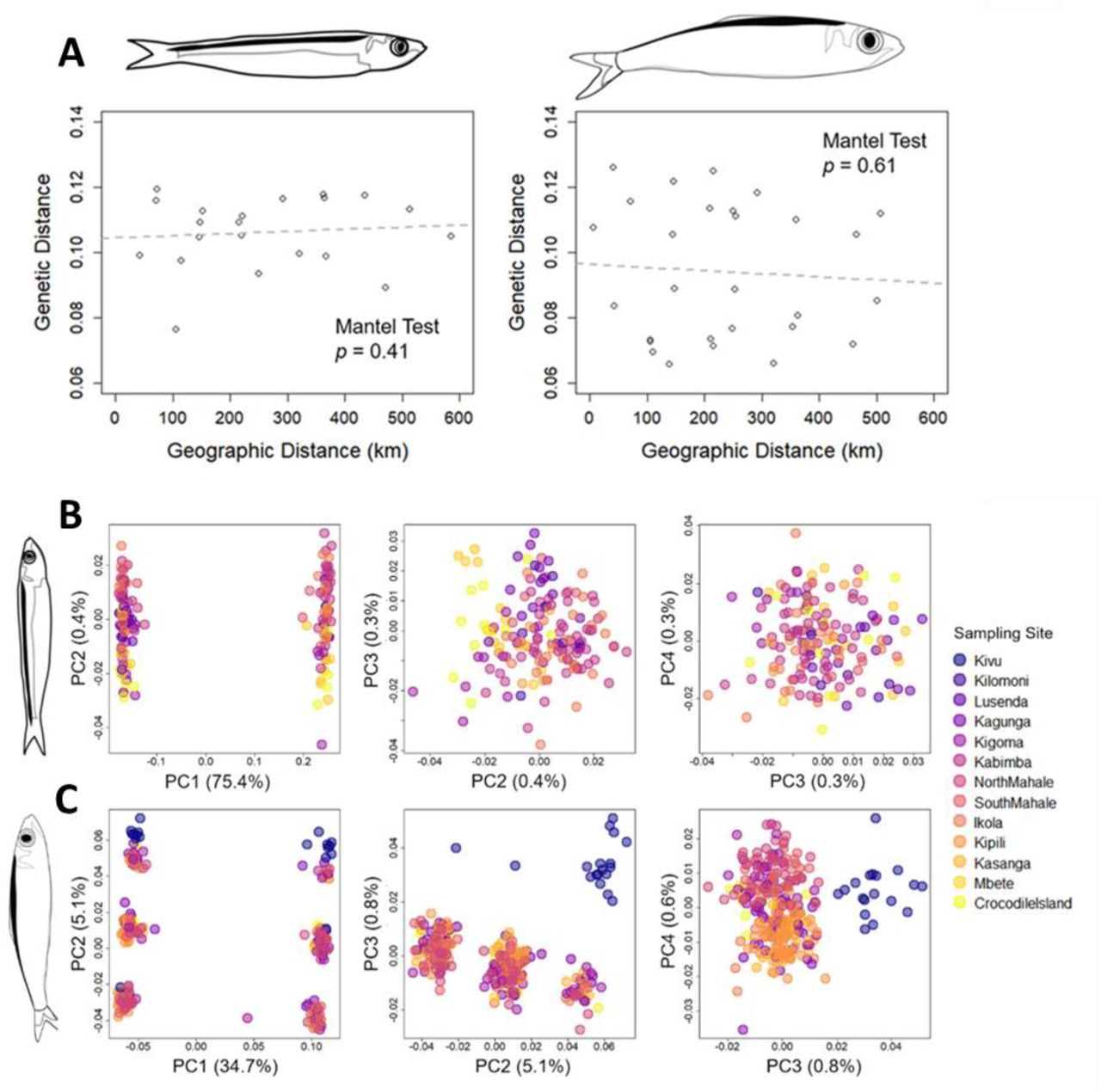
(A) shows the relationship between genetic and geographic distance. Neither species has evidence for statistically significant spatial population genetic structure using mantel test. (B) and (C) show Species-specific principal components analysis of Stolothrissa and Limnothrissa individuals, colored by sampling sites. In both species, PC1 differentiates the sexes; in Limnothrissa, PC2 separates each sex into three distinct groups, while PC3 separates individuals from Lake Kivu from those in Lake Tanganyika. Sampling sites are ordered from north (Kivu) to south (Crocodile Island).
Genetic diversity within (Watterson’s theta, ΘW, along diagonal) and differentiation between (weighted FST, above diagonal) sampling sites (unshaded) and basins (shaded) for Limnothrissa populations included in this study.
Genetic diversity within (Watterson’s theta, ΘW, along diagonal) and differentiation between (weighted FST, above diagonal) sampling sites (unshaded) and basins (shaded) for Stolothrissa populations included in this study.
Evidence for a segregating inversion in Limnothrissa
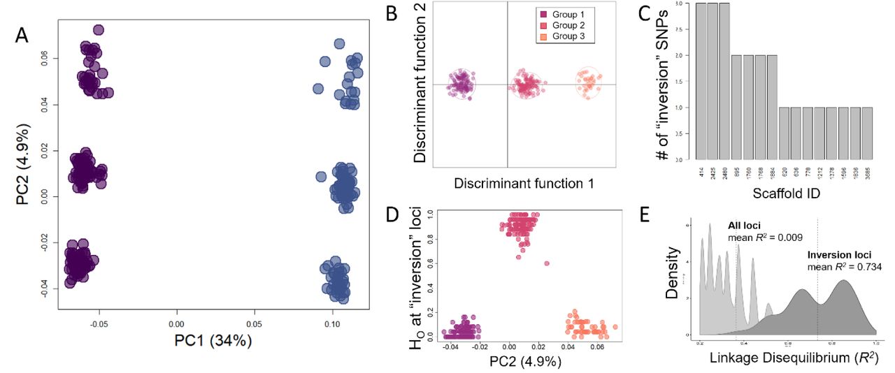
Limnothrissa from Lake Kivu are divergent from individuals in Lake Tanganyika, but this differentiation is weaker than that between the three groups observed within Lake Tanganyika (Fig 3C). The Limnothrissa individuals from Lake Kivu form additional clusters that are distinct from, but parallel to, the Tanganyika clusters along the second and third PC axis (Fig 3C). Within Lake Tanganyika, we found individuals of all three clusters at single sampling sites, and there is no clear geographic signal to these groups (Fig 3C). DAPC analysis of the two most differentiated groups within Lake Tanganyika identified 25 SNPs across 15 scaffolds with high loadings (> 0.006; Fig 4C and S3). Among these SNPs with high loadings, we found that two clusters of Limnothrissa individuals were predominantly homozygous for opposite alleles, while the third group consisted of heterozygotes at these loci (Fig. 4D). This suggests that the three distinct genetic groups we observe are due to a segregating inversion, with two of the groups representing homokaryotypes and the third a heterokaryotype for these SNPs (Fig 4 and S3).

Evidence in Limnothrissa points to the existence of a segregating inversion. (A) Principal component analysis for all Limnothrissa individuals of Lake Tanganyika, demonstrating separation among sexes along the first principal component axis (PC1), and separation into three groups for both males (purple) and females (blue) on the second axis (PC2). For our discriminant analysis of principal components (B), we identified individuals according to these groups, and identified SNPs with high loadings along this axis. (C) Scaffold locations of SNPs with high loadings along this ‘group’ axis, showing that the 25 significant SNPs were found on 15 different scaffolds. At these significant loci, two groups were predominantly homozygous (D), while the third (intermediate) group was generally heterozygous. Despite the fact that these SNPs were spread out across several scaffolds, the distribution of pairwise linkage disequilibrium values (E) between just the inversion loci (dark) has a mean R2 = 0.734, whereas the distribution for all loci in the data set for Limnothrissa (light) has a mean R2 = 0.009.
With this suggestion of a segregating inversion within Limnothrissa, we tested for Hardy-Weinberg equilibrium among the three groups within the lake as a whole and at each sampling site individually (Fig 5). In Lake Tanganyika, all sampling sites, regions, and the lake as a whole were in HWE (X2, p > 0.05), while Lake Kivu frequencies differed significantly from HWE (X2, p = 0.005) (Fig 5A and 5B). We additionally found that the proportions of all three karyotype groups differed significantly between Lake Kivu fish and the fish found in each of the north, middle (Mahale), and south basins in Lake Tanganyika (p = 0.012, p = 0.0036, p << 0.001) (Fig 5B). This result seems to be driven by a much higher frequency of genotype group 3 in Lake Kivu samples than was found in Lake Tanganyika (Fig 5B). The only difference between the three basins within Lake Tanganyika was that the northern basin had a greater frequency of fish with genotype group 3 than either the Mahale or southern basins (p = 0.025; all others p > 0.05) (Fig 5B).

Proportion of individuals in each inversion karyotype group, by sampling site (A) and region (B). Sample sizes of individuals retained in analyses at each sampling site are indicated, as well as whether the distribution of the groups at each site differs from expectations under Hardy-Weinberg equilibrium (* indicates rejection of HWE at the site). Sites are ordered by geographic location, from north (Kivu, Kagunga) to south (Crocodile Island). The relative proportions of each haplotype observed differed significantly between Lake Kivu and all three regions in Lake Tanganyika, while only the relative proportion of Group 3 differed among the three regions within Lake Tanganyika.
Linkage disequilibrium among identified loci
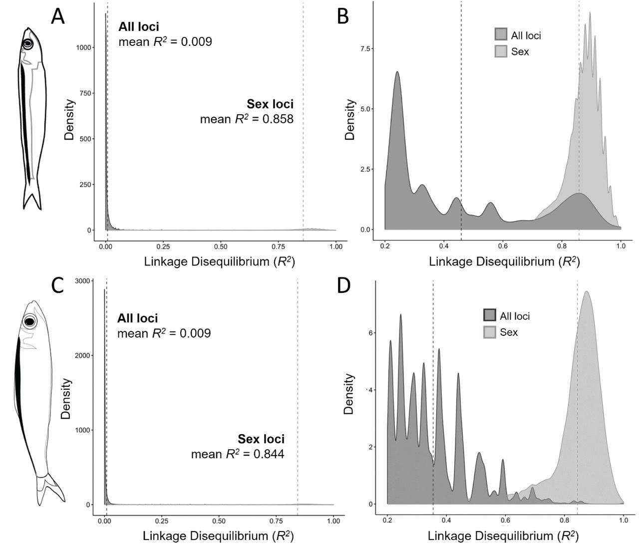
The distribution of pairwise linkage disequilibrium values among loci in the species-specific and species-combined datasets were highly right-skewed, with the majority of loci pairs having low to no linkage (mean R2 = 0.009) (Fig 6). In contrast, the subsets of loci identified as sex-linked in Stolothrissa and Limnothrissa had mean pairwise LD values of 0.858 and 0.844, respectively (Fig 6), suggesting that these sets of loci are more tightly linked than expected based on the distribution of LD values for all loci (Mann-Whitney test; Stolothrissa W = 1167300000, p << 0.001; Limnothrissa W = 202550000, p << 0.001). In Limnothrissa, the group-delineating loci had a mean pairwise LD of 0.734, suggesting that they are also more linked than expected for random loci (Mann-Whitney test, W = 23862000000, p << 0.001), but less tightly linked than the sex-linked loci (Mann-Whitney test, W = 1862600, p << 0.001).

Results from an analysis of pairwise linkage disequilibrium (measured as R2) between SNPs in Stolothrissa (A-B) and Limnothrissa (C-D), demonstrating that loci associated with sex differences (light gray distributions) are more tightly linked than expected based on linkage values for all loci in the species-specific data sets (dark gray distributions). Panels (C) and (D) have been truncated at R2 = 0.2 to better visualize the distribution of LD values for sex-associated SNPs.
No overlap of sex linked loci in the two sardine species
To test if the sex-linked loci overlap between the species, we used the species-combined dataset to perform DAPC between sexes for each species individually and identified loci with high loadings. Using this approach, we identified 570 SNPs across 133 scaffolds in Stolothrissa (loading > 0.0006; Fig S4) and 334 SNPs across 91 scaffolds in Limnothrissa linked to sex (loading > 0.001; Fig S5). These two sets of loci were completely non-overlapping, suggesting that the sex-linked loci are unique in each species. In addition, the scaffolds on which these loci were located were non-overlapping between the species, suggesting that the discrepancy between identified loci is not simply due to different coverage of the reference genome between Stolothrissa and Limnothrissa data. When looking at Stolothrissa sex-linked SNPs in Limnothrissa individuals, only 2.5% are polymorphic, and only 0.8% of Limnothrissa sex-linked SNPs are polymorphic in Stolothrissa. In addition, the sex loci for each species do not show the same patterns of heterozygosity in the opposite species (Fig S6).
Discussion
Little to no spatial genetic structuring is a relatively common observation in pelagic fish species with continuous habitats (e.g. Canales-Aguirre et al. 2016; Hutchinson et al. 2001; Momigliano et al. 2017). However, many studies show that pelagic fish species harbour genetic structure that does not correspond with geographic distance, but instead correlates with ecological adaptation (Berg et al. 2017; Kirubakaran et al. 2016; Roesti et al. 2015). We present here the largest genomic data sets analysed for the two freshwater sardines of Lake Tanganyika to date. We did not find evidence for spatial genetic structure in Stolothrissa or Limnothrissa of Lake Tanganyika (Fig 3), despite the immense size of this lake and extensive geographic sampling of populations of both species. Instead, we find evidence for the existence of many sex-linked loci in both Stolothrissa and Limnothrissa, including strong deviations from expected heterozygosity at these loci, with males being the heterogametic sex (Fig 2). In Limnothrissa, we additionally find three cryptic genetic groups, and patterns in heterozygosity indicate the presence of a segregating chromosomal inversion underlying this genetic structure (Fig 4). All three inversion genotypes (homokaryotypes and heterokaryotype) appear in Limnothrissa from both Lake Tanganyika and Lake Kivu, but relative frequencies of the karyotypes differ among these populations (Fig 5).
Genetic sex differentiation in both species
According to the canonical model of sex chromosome evolution, development of sex chromosomes initiates with the appearance of a sex-determining allele in the vicinity of loci only favourable for one of the sexes. Mechanisms reducing recombination, such as inversions, support the spread of the sex-determining allele in combination with the sexually antagonistic region due to high physical linkage. Eventually neighbouring regions also reduce recombination rate and further mutations accumulate, leading to the formation of a new sex chromosome (Bachtrog 2013; Gammerdinger & Kocher 2018; Wright et al. 2016). Examples range from ancient, highly heteromorphic sex chromosomes, to recent neo-sex chromosomes, which are found in mammals (Cortez et al. 2014), avian species (Graves 2014), and fishes (Feulner et al. 2018; Gammerdinger et al. 2018; Gammerdinger & Kocher 2018; Kitano & Peichel 2012; Pennell et al. 2015; Roberts et al. 2009; Ross et al. 2009; Yoshida et al. 2014). Our results suggest that sex-linked regions of the genome in both Stolothrissa and Limnothrissa are large and highly differentiated between males and females (Fig. 2). The results from our analyses of linkage disequilibrium suggest that these loci are more tightly linked in both Limnothrissa and Stolothrissa than SNP loci are on average (Fig 6). The high number of loci implicated in these genetic sex differences, and high linkage among those loci, in addition to clear patterns of excess heterozygosity in males and homozygosity in females, give strong indication of the existence of large sex-determining regions in these species, which may form distinct sex chromosomes. However, the structural arrangement of these loci remains unclear with our current reference genome. It is worth noting that the assembly of sex chromosomes remains challenging due to the haploid nature of sex chromosomes and therefore reduced sequencing depth, and existence of ampliconic and repetitive regions and a high amount of heterochromatin (Tomaszkiewicz et al. 2017). Such challenges with assembling sex chromosomes may lead to many scaffolds being implicated in sex determination in initial attempts at assembly, as we see in our analysis, even if these species actually have distinct sex chromosomes.
We also show that Stolothrissa and Limnothrissa SNPs linked to sex are entirely distinct, representing strong evidence for rapid evolution in these sex-linked regions (Fig S1 and S2). This means that if the common ancestor of these species had a sex-determining region, the variants on this sex-linked region have entirely turned over and become distinct in the two species, during the approximately eight million years since these species diverged (Wilson et al. 2008). Rapid turnover of sex chromosomes in closely related species are known from a diversity of taxa (e.g. (Jeffries et al. 2018; Kitano & Peichel 2012; Ross et al. 2009; Tennessen et al. 2018). The proposed mechanisms leading to such rapid turnover rates are chromosomal fusions of an autosome with an already existing sex chromosome, forming a “neo sex chromosome” (Kitano & Peichel 2012; Ross et al. 2009) or the translocation of sex loci from one chromosome to another (Tennessen et al. 2018). Understanding the mechanisms responsible for the high turnover rate of the sex chromosomes in the Tanganyikan freshwater sardines is a fascinating area for future research.
Furthermore, it will be important for future work to investigate if the strong differentiation between the sexes might also be associated with adaptive differences between the sexes. Ecological polymorphism among sexes is known in fishes (Culumber & Tobler 2017; Laporte et al. 2018; Parker 1992) and can be ecologically as important as differences between species (Start & De Lisle 2018). It is worth noting that the strong sex-linked genetic differentiation in Limnothrissa and Stolothrissa could have been mistaken for population structure had we filtered our data for excess heterozygosity without first examining it, and had we not been able to carefully phenotypically sex well-preserved, reproductively mature individuals of both species to confirm that the two groups in each species do indeed correspond to sex (Table S1, Fig 2A). Because of the strong deviations from expected heterozygosity at sex-linked loci, any filtering for heterozygosity would remove these loci from the dataset, explaining why one previous study in Stolothrissa using RADseq data (De Keyzer et al. 2019) did not clearly identify this pattern despite its prevalence in the genome. For organisms with unknown sex determination systems, and for whom sex is not readily identifiable from phenotype, there is danger in conflating biased sampling of the sexes in different populations with population structure in genomic datasets (e.g. Benestan et al. 2017). This underscores the importance of sexing sampled individuals whenever possible when sex determination systems are unknown, when analyzing large genomic datasets. The phenotypic and genetic sex of the sardine samples were in agreement in all individuals except one Stolothrissa sample (Table S1, sample 138863.IKO02). This fish was phenotypically identified as a male but genetically clustered with female individuals. We believe that this individual was not yet fully mature, and therefore was misidentified phenotypically.
No spatial genetic structure in Limnothrissa but cryptic diversity in sympatric Limnothrissa
Our results reveal the existence of three distinct genetic groups of Limnothrissa. Intriguingly, we find all three of these groups together within the same sampling sites, and even within the same single school of juvenile fishes (Fig S7). Given patterns of heterozygosity at loci that have high loadings for distinguishing among the genetic clusters (Fig 4D) together with the strong linkage (Fig 4E), this structure is consistent with a chromosomal inversion. Chromosomal inversions, first described by Sturtevant (1921), reduce recombination in the inverted region because of the prevention of crossover in heterogametic individuals (Cooper 1945; Kirkpatrick 2010; Wellenreuther & Bernatchez 2018). Mutations in these chromosomal regions can therefore accumulate independently between the inverted and non-inverted haplotype. Although early work on chromosomal inversions in Drosophila has a rich history in evolutionary biology (Kirkpatrick 2010), inverted regions have recently been increasingly detected with the help of new genomic sequencing technologies in many species (e.g. Berg et al. 2017; Christmas et al. 2018; Kirubakaran et al. 2016; Lindtke et al. 2017; Zinzow-Kramer et al. 2015), with implications for the evolution of the populations with distinct inversion haplotypes. In Limnothrissa, the strong genetic divergence between the two inversion haplotypes (Fig 3C, 4A and 4B) is consistent with this pattern, and indeed the substantial independent evolution of these haplotypes is how the inversion is readily apparent even in a RADseq dataset. The divergence of the haplotypes, and the high frequency of both of these haplotypes, indicates that this inversion likely did not appear recently, although its apparent absence in Stolothrissa indicates it has arisen since the divergence of these sister taxa eight million years ago (95% reliability interval: 2.1–15.9 MYA; (Wilson et al. 2008)).
Given that both inversion haplotypes appear in relatively high numbers, it seems unlikely that drift alone could explain the rise of the inversion haplotype to its current frequencies in the Limnothrissa population. We expect that Limnothrissa have sustained large effective population sizes through much of their evolutionary history since their split with Stolothrissa, meaning that drift would have been a continually weak force. Although selection against inversions might occur due to an inversion’s disruption of meiosis or gene expression due to the position of the breakpoints (Kirkpatrick 2010), selection may also act on inversions when they carry alleles that themselves are under selection.
Due to the reduced recombination rates in inversions, these regions of the genome provide opportunities for local or ecological adaptation despite ongoing gene flow (Kirkpatrick & Barton 2006). It is unclear given current data whether the inversion that we describe here in Limnothrissa is tied to differential ecological adaptation. When we examine frequencies of the inversion karyotypes pooled across all sampled populations, the observed frequencies do not differ from Hardy-Weinberg expectations (chi-square = 3.51; p-value = 0.06). However, the Lake Kivu population does show deviation from HWE (chi-square =7.74; p-value = 0.005) when we examine sampled populations individually. Furthermore, frequencies of the inversion karyotypes among sampled populations differ: the proportions of all three karyotypes differ significantly between Lake Kivu and Lake Tanganyika populations, and within Lake Tanganyika, one of the homokaryotypes (represented as group 3 in Fig 5), has a higher frequency in the northern basin than in the middle or southern basins (Fig 5). In Lake Tanganyika, the southern and northern basin differ substantially in nutrient abundance and limnological dynamics, and the Mahale Mountain (middle) region represents the geographical transition between the two basins (Bergamino et al. 2010; Kraemer et al. 2015; Plisnier et al. 1999; Plisnier et al. 2009). Thus, it is plausible that differential ecological selection could be driving differences in the frequencies on the inversion karyotypes spatially within the lake. Genetic drift is another possibility to explain the spatial differences in frequencies, and although this is highly plausible in explaining the frequency differences between Lake Tanganyika and Lake Kivu (see below), given the lack of spatial genetic structure in Lake Tanganyika it seems a less likely explanation within this lake. Greater understanding of the ecology of these fishes in the north and the south of Lake Tanganyika, and assessment of the genes within the inverted region, is needed to clarify this question.
Comparing Limnothrissa populations in Lake Tanganyika to that introduced to Lake Kivu
We found substantial divergence between Limnothrissa in their native Lake Tanganyika and the introduced population in Lake Kivu. This could derive from founder effects, from drift within this population since their introduction in the absence of gene flow with the Lake Tanganyika population, or from adaptive evolution in the Lake Kivu population since their introduction to this substantially different lake environment. Future studies should examine these possibilities with a larger sample of individuals from Lake Kivu. We identified individuals in Lake Kivu with all three inversion genotypes that were detected in Lake Tanganyikan fish, suggesting that the inversion is also segregating in Lake Kivu, and that the founding individuals likely harboured this genetic variation. That said, the frequency of the karyotypes in Lake Kivu strongly deviates from Hardy-Weinberg expectations (Chi-square =7.74; p-value =0.005). This suggests that the inversion locus may be under directional selection. This finding is in contrast with frequent expectations for the behaviour of inversions: typically, one would predict some sort of balancing selection (e.g. negative frequency dependent selection) to maintain inversion haplotype diversity (Wellenreuther & Bernatchez 2018). Another possibility is that the inversion locus is linked to non-random mating in the Kivu population. In addition, the strong difference in the frequencies of the inversion haplotypes compared to Lake Tanganyika populations has also likely been influenced by founder effects. Limnothrissa were introduced to Lake Kivu in the 1950s (Hauser et al. (1995), and all introduced fish were brought from the northern part of Lake Tanganyika. The homokaryotype, represented as group 3, is the prevalent karyotype in Lake Kivu, and this karyotype also appears in highest frequencies in our samples from northern Lake Tanganyika sites (Fig 5). Thus, it is plausible that founder effects could have led to the increased frequency of this karyotype within the Lake Kivu population. This origin, however, does not explain current deviations from HWE given that the population was introduced decades ago.
Conclusions
Genomic data from Stolothrissa and Limnothrissa reveal an interesting array of unexpected patterns in chromosomal evolution. Modern fisheries management seeks to define locally adapted, demographically independent units. We do not find significant spatial genetic structure within these two freshwater sardine species from Lake Tanganyika. The genetic structure we find is all in sympatry, namely as strong genetic divergence between the sexes, and evidence of a segregating inversion in Limnothrissa. Further research should focus on the potential for adaptive differences between the sexes and between the inversion genotypes in Limnothrissa. Such work will contribute to better understanding the role that these key components of the pelagic community assume in the ecosystem of this lake, which provides important resources to millions of people living at its shores.
Data Accessibility Statement
We are happy to make our genetic data, including our reference genome, publically available by submitting it to the European Nucleotide Archive (ENA). We intend to submit as soon as possible but by the latest after acceptance of the manuscript.
Data Accessibility
- RAD sequences: will be uploaded to ENA as soon as possible but by the latest after acceptance
- Final DNA sequence assembly will be uploaded to ENA as soon as possible but by the latest after acceptance
Author contributions
JJ: developing and writing SNSF grant, sampling and processing fish, identifying phenotypic sex of fish, DNA extractions, preparing RAD libraries, data analysis, writing on the manuscript
JR: sampling and processing fish, DNA extractions, whole genome assembly, data analysis, writing on the manuscript
PBM: developing grant for The Nature Conservancy, contributing samples, discussing results, reviewing manuscript
IK: developing and writing SNSF grant, facilitating permission processes, providing logistics for fieldwork, reviewing manuscript
EAS: sampling and processing fish, facilitating permission processes, providing logistics for fieldwork, enable collaboration with Tanzanian fishermen, discussing manuscript, reviewing manuscript
JBM: sampling and processing fish, facilitating permission processes, providing logistics for fieldwork, enable collaboration with Tanzanian fishermen, discussing and reviewing manuscript
BW: developing and writing SNSF grant, reviewing and discussing manuscript
CD: developing SNSF grant, sampling and processing fish, facilitating logistics during fieldwork, reviewing manuscript
SM: developing SNSF grant, facilitating permission process, RAD library preparation for sequencing, reviewing manuscript
OS: developing and writing SNSF grant, identifying phenotypic sex of fish, facilitating permission process, reviewing and discussing manuscript
CEW: developing and writing SNSF and TNC grants, sampling and processing fish, contributing samples, whole genome assembly, data analysis, discussing results, writing manuscript, revise manuscript
Acknowledgements
This work was funded by the Swiss National Science Foundation (grant CR23I2-166589), a grant from The Nature Conservancy to CEW and PBM, and start-up funding from the University of Wyoming to CEW. CEW was partially supported by NSF grant DEB-1556963. Computing was accomplished with an allocation from the University of Wyoming’s Advanced Research Computing Center, on its Teton Intel x86_64 cluster (https://doi.org/10.15786/M2FY47) and the Genetic Diversity Center (GDC) of ETH Zürich. Special thanks go to Mupape Mukuli, for facilitating logistics during fieldwork and to the crew of the MV Maman Benita. We thank the whole team at the Tanzanian Fisheries Research Institute for their support. A special thank goes to Mary Kishe for her support during fieldwork permission processes and to the Tanzanian Commission for Science and Technology (COSTECH) for their support of this project through permits allowing us to do research in Tanzania. Thanks to Mark Kirkpatrick and his lab group for enlightening discussion regarding the interpretation of these data, and to the Wagner lab at the University of Wyoming, and the FishEc group at EAWAG, especially Kotaro Kagawa and Oliver Selz, for helpful discussion.
References


