

Abstract
Live-cell imaging experiments have opened an exciting window into the behavior of living systems. While these experiments can produce rich data, the computational analysis of these datasets is challenging. Single-cell analysis requires that cells be accurately identified in each image and subsequently tracked over time. Increasingly, deep learning is being used to interpret microscopy image with single cell resolution. In this work, we apply deep learning to the problem of tracking single cells in live-cell imaging data. Using crowdsourcing and a human-in-the-loop approach to data annotation, we constructed a dataset of over 11,000 trajectories of cell nuclei that includes lineage information. Using this dataset, we successfully trained a deep learning model to perform cell tracking within a linear programming framework. Benchmarking tests demonstrate that our method achieves state-of-the-art performance on the task of cell tracking with respect to multiple accuracy metrics. Further, we show that our deep learning-based method generalizes to perform cell tracking for both fluorescent and brightfield images of the cell cytoplasm, despite having never been trained on those data types. This enables analysis of live-cell imaging data collected across imaging modalities. A persistent cloud deployment of our cell tracker is available at http://www.deepcell.org.
Introduction
Live-cell imaging experiments, where living cells are imaged over time with fluorescence or brightfield microscopy, has provided crucial insights into the inner workings of biological systems. To date, these experiments have shed light on numerous problems, including information processing in signaling networks1–3 and quantifying stochastic gene expression4–7. One key strength of live-cell imaging experiments is the ability to obtain dynamic data with single-cell resolution. It is now well appreciated that individual cells can vary considerably in their behavior, and the ability to capture the temporal evolution of cell-to-cell differences has proven essential to understanding cellular heterogeneity. Increasingly, these dynamic data are being integrated with end-point genomic assays to uncover even more insights into cellular behavior8–10.
Central to the interpretation of these experiments is image analysis. Traditionally, the analysis of these data occurs in three phases. First, images are cleaned with steps that include background subtraction and drift correction. Next, the image is segmented to identify each individual cell in every frame. This segmentation step can capture the whole cell or cellular compartments like the nucleus. Lastly, all the detections for an individual cell are linked together in time to form a temporally cohesive record for each cell; a schematic of this step is shown in Figure 1(a). With a suitable algorithm and data structure, these records can contain lineage information such as parent-child relationships for each cell. The output of this analysis pipeline is a record for each cell of which pixels are associated with it in each frame of the dataset as well as lineage information. This record can then be used to obtain quantitative information – ranging from metrics of cellular morphology to fluorescence intensity – over time.

Tracking single cells with deep learning and linear programming. (a, b) Computational analysis is a significant barrier for extracting single cell information from movies of living cells. Cells must be identified in every frame and then these detections must be linked together over time to form a temporal record for each cell. (c) Cell tracking can be framed as a linear assignment problem in which Ni objects in frame i are matched up with Ni+1 objects in frame i+1. Shadow objects can be introduced to account for births (i.e. from cell division events) or deaths (i.e. cells leaving the field of view). Solving the linear assignment problem requires first creating a cost matrix that scores each possible assignment. The Hungarian algorithm34 is then used to find the optimal assignment that minimizes the cost function. Instead of manually engineering this cost function, we use a deep learning model to learn one from annotated data. Here, psame is the probability that two cells being compared are the same, b is the cost associated with cell “births” (i.e. a cell in frame i+1 being assigned to a shadow cell), and d is the cost associate with a cell death (i.e. a cell in frame i being assigned to a shadow cell). A deep learning model learns to take information from two cells and compute the probability these are the same cell, different cells, or have a parent-child relationship. This model takes information on each cell’s appearance, local neighborhood, morphology, and motion and summarizes as a vector using a deep learning sub-model. A fully connected layer reads these summaries and determines the scores for the three classes.
Advances in imaging technologies – both in microscopes11 and fluorescent reporters12 – have significantly reduced the difficulty of acquiring live-cell imaging data while at the same time increasing the throughput and the number of systems amenable to this approach. Increasingly, image analysis is a bottleneck for discovery as there is a gap between our ability to collect and analyze data. This gap can be traced to the limited accuracy and generality of cell segmentation and tracking algorithms. These limitations lead to a significant curation time, recently estimated to be >100 hours for one manuscript worth of data13. Recent advances in computer vision, specifically deep learning, are closing this gap14. For the purposes of this paper, deep learning refers to a set of machine learning methods capable of learning effective representations from data in a supervised or unsupervised fashion. Deep learning has shown a remarkable ability to extract information from images and it is increasingly being recognized that it is a natural fit for the image analysis needs of the life sciences15,16. As a result, deep learning is increasingly being applied to biological imaging data – applications include using classification to determine cellular phenotypes17, enhancing image resolution18, and extracting latent information from brightfield microscope images19,20. Of interest to those who use live-cell imaging has been the application of this technology to single-cell segmentation. The popular deep learning model architecture U-Net targeted cell segmentation as its first use case21,22 and our group’s prior work has shown that deep learning can perform single-cell segmentation for organisms spanning the domains of life as well as in images of tissues13,23. Recent approaches have extended these methods to 3D datasets24. The improved accuracy of single-cell segmentations for live-cell imaging is crucially important, as a single segmentation error in a single frame can impair subsequent attempts at cell tracking and render a cell unsuitable for analysis.
While deep learning has been successfully applied to single-cell segmentation, a robust deep learning-based cell tracker for mammalian cells has been elusive. Integration of deep learning into live-cell imaging analysis pipelines achieve performance boosts by combining the improved segmentation accuracy of deep learning with conventional object tracking algorithms13,25–27. These algorithms include linear programming28 and the Viterbi algorithm29; both have seen extensive use on live-cell imaging data. While useful, these object tracking algorithms have limitations. Common events that lead to tracking errors include cell division and cells entering and leaving the field of view. Furthermore, their use often necessitates tuning numerous parameters to optimize performance for specific datasets, which leads to fragility on unseen data. Though there have been attempts at adapting deep learning to track cells30, their performance is significantly limited by a lack of training data, as fine-tuned conventional methods still achieve superior performance.
Three technical challenges have impeded the creation of a readily available, deep learning-based cell tracker. First, as previously mentioned, the unique features of live-cell imaging data (i.e. cell divisions) confound traditional tracking methods as well as deep learning-based object trackers. Second, successful deep learning solutions are data hungry. While unsupervised deep learning can be a useful tool, most applications of deep learning to imaging data are supervised and require significant amounts of specialized training data. Aggregating and curating training data for tracking is especially difficult because of the additional temporal dimension – objects must be segmented and tracked through every frame of a training dataset. Third, deep learning’s requirement for hardware acceleration presents a barrier for performing large inference tasks. On premise computing has limited throughput, while cloud computing poses additional software engineering challenges.
In this paper, we address each of these challenges to construct an effective deep learning-based solution to cell tracking in two dimensional live-cell imaging data. We show how cell tracking can be solved with deep learning and linear programming. We then demonstrate how a combination of crowdsourcing and human-in-the-loop data annotation can be used to create a live-cell imaging training dataset consisting of over 11,000 single cell trajectories. We benchmark the resulting tracker using multiple metrics and show it achieves state-of-the-art performance on several datasets, including data from the ISBI cell tracking challenge. Lastly, leveraging our prior work with cloud computing31, we show how our cell tracker can be integrated into the DeepCell 2.0 single-cell image analysis framework to enable segmentation and tracking live-cell imaging datasets through their web browser.
Tracking single cells with deep learning and linear programming
Our approach to cell tracking is motivated by the now classic work of Jaqaman et al32 and recent work applying deep learning to object tracking33. In these works, object tracking is treated as a linear assignment problem (Figure 2a). In this framework, Ni objects in frame i must be assigned to Ni+1 objects in frame i+1. To solve this assignment problem, one constructs a cost function for a possible pairing across frames, which is traditionally based on each object’s location and appearance features (brightness, size, etc.)28. The guiding intuition is that objects are unlikely to move large distances or have distinct changes in appearance from frame-to-frame if the frame rate is sufficiently high. The problem is then reduced to the selection of one assignment out of the set of all possible assignments that minimizes the cost function, a task that can be accomplished with the Hungarian algorithm34. One complicating factor of biological object tracking is that objects can appear and disappear – this often leads to Ni and Ni+1 being unequal. This problem can be solved by introducing a “shadow object” for each object in the two frames32 – Ni+1 shadow objects in frame i and Ni shadow objects in frame i+1. These shadow objects represent an opportunity for objects to “die” (if an object in frame i is matched with its shadow object in frame i+1) or to be “born” (if an object in frame i+1 is matched with its shadow object in frame i). This framework leads to a cost matrix describing the cost of every possible assignment that is size Ni + Ni+1 x Ni + Ni+1; its structure is shown in Figure 2a.

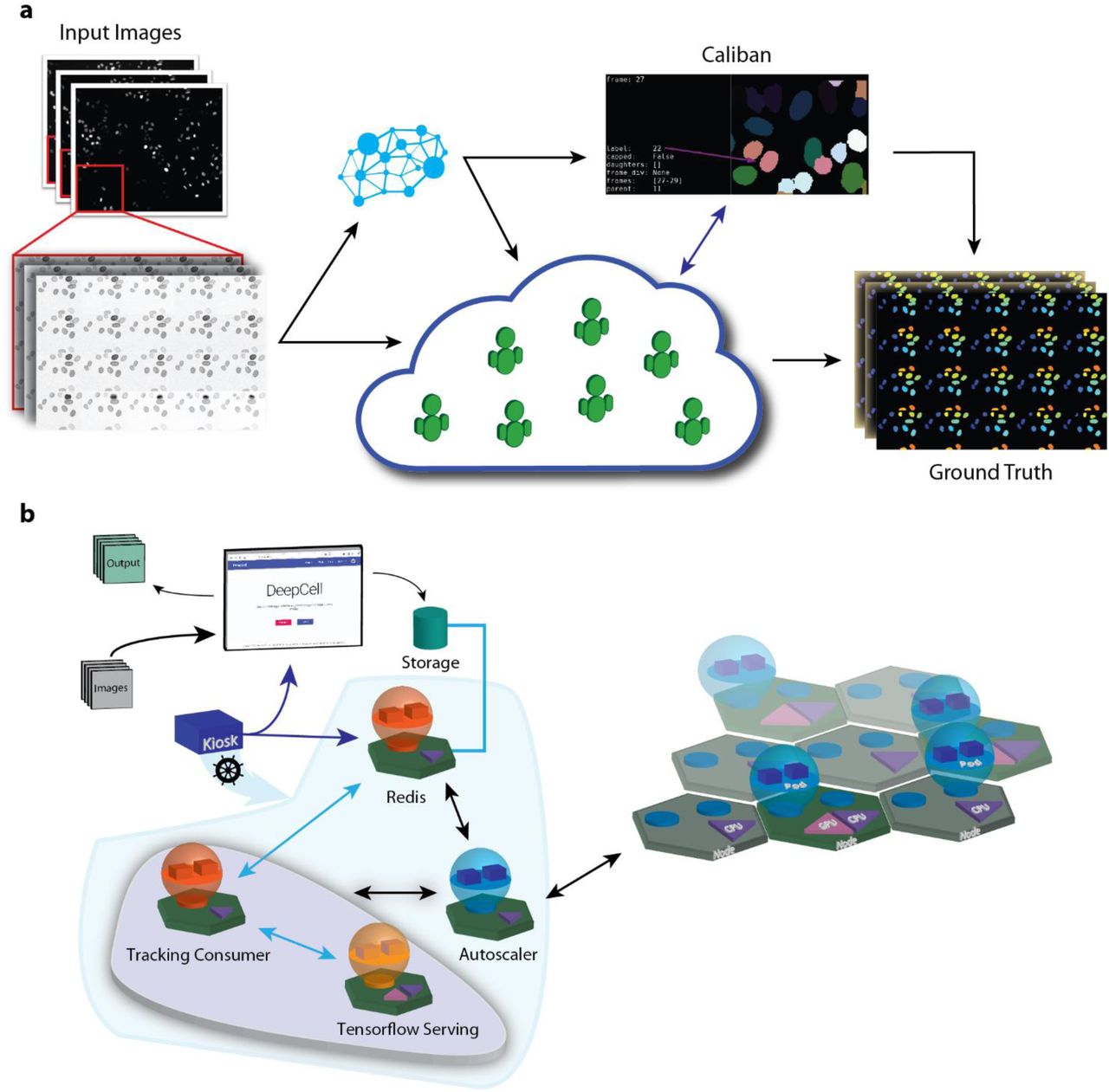
A human-in-the-loop to dataset construction and cloud computing facilitate a scalable solution to live-cell image analysis. (a) Combining crowd sourcing and a human-in-the-loop approach to dataset annotation enables the construction of an ImageNet for live-cell imaging. By annotating montages, crowd contributors both segment and track single cells in live-cell imaging data. This data leads to models that are used to process additional data; expert annotators use Caliban to correct model errors and identify cell division events. The resulting data is then used to train a final set of deep learning models to perform cell segmentation and tracking. (b) Integration of a cell tracking service into DeepCell 2.0. Datasets are uploaded to a cloud bucket; once there, a tracking consumer object facilitates interactions with deep learning models via Tensorflow serving for segmentation and tracking. The implementation within the Kubernetes engine includes an autoscaling module that monitors resource utilization and scales the compute resources accordingly.
Assuming error-free image segmentation and an accommodation for dealing with cell divisions, cell tracking can fit neatly into this framework. Whole movies are tracked by sequentially tracking every pair of frames – this is to be contrasted with approaches like the Viterbi algorithm that incorporate multiple frames worth of information to determine assignments. One advantage of this approach is that it can cope with missing objects – instead of using the objects in frame i for comparison, we instead compare all objects that have been successfully tracked up to frame i. If objects disappear and reappear, the opportunity to correctly track them still exists. Optimization of the linear assignment approach’s performance on real data comes about through cost function engineering. By varying key aspects of the cost function – how sensitive it is to the distance between two cells, how much it weights the importance of cell movement vs cell appearance, etc. – it is possible to tune the approach to have acceptable performance on live-cell imaging datasets. However, this approach has several downsides – the accuracy is limited, the time required for cost function engineering and curation of results is prohibitive, and solutions are tailored to specific datasets which reduces their generality.
Here, we take a supervised deep learning approach to learn an optimal cost function for the linear assignment framework. Our approach was inspired by previous work applying deep learning to object tracking33. Building on this work, we make adaptations to deal with the unique features of live-cell imaging data (Figure 1c). To construct our learned cost function, we consider it as a classification task. Let us suppose we have two cells – cell 1 in frame i and cell 2 in frame i+1. Our goal is to construct a classifier that would take in information about each cell and produce a probability that these two cells are either the same, are different, or have a parent-child relationship. If such a classifier worked perfectly, then we could use it in lieu of our hand engineered cost function, as is shown in Figure 2b. To incorporate temporal information, we can use multiple frames of information for cell 1 as an input to the classifier. This allows us access to the temporal information beyond just the two frames we are comparing. For our work here, we use 7 frames worth of information.
Our classifier for performing this task is a hybrid recurrent-convolutional deep learning model; its architecture is shown in Figure 1c. This deep learning model takes in 4 pieces of information about each cell using 4 separate branches. Conceptually, each branch seeks to summarize its input information as a vector. These summary vectors can then be fed into a fully connected neural network to classify the two cells being compared. The first branch takes in the appearance, that is a cropped and resized image, of each cell and uses a deep convolutional neural network to generate a summary. This network is applied to every frame for cell 1, creating a sequence of summary vectors. Conversely, cell 2 only has 1 frame of information and hence only has 1 summary vector. The appearance gives us access to information on what the two cells look like, but the resizing operation removes notions of size scale. To mitigate this, we incorporate a second branch that takes in a vector of morphological information for each cell and uses a densely connected neural network to create a summary vector of this information. The morphology information used includes the area, perimeter, and eccentricity. The third branch acquires information about cell motion over time. For cell 1, we collect a vector of all the centroid displacements. For cell 2, we create a single vector that is the displacement between cell 1 and cell 2’s centroid. This branch gives us a history of cell 1’s motion and allows us to see whether a potential positive assignment of cell 2 would be inconsistent from the point of view of cell motion. The last branch incorporates neighborhoods, which is an image cropped out around the region surrounding cell 1. We reasoned that because neighborhoods contain information about cell divisions, they could prove useful in performing lineage assignments. Just as with appearances, a deep convolutional neural network is used to summarize the neighborhoods as a vector. We extract the neighborhood around the area cell 1 is predicted to be located given cell 1’s velocity vectors and use it as the neighborhood for cell 2. The result of these 4 branches are sequences of summary vectors for cell 1 and individual summary vectors for cell 2. Long short-term memory (LSTM) layers are then applied to each of cell 1’s sequence of summary vectors to merge the temporal information and create 4 individual vectors that summarize each of the 4 branches. The vectors for cell 1 and cell 2 are then concatenated and fed into fully connected layers. The final layer applies the softmax transform to produce the final classification scores – psame, pdiff, and pparent-child. These three scores, which are all positive and sum to 1, can be thought of as probabilities. They are used to construct the cost matrix, as shown in Figure 2b. If a cell in frame i+1 is assigned to a shadow cell, i.e. it is “born,” then we check whether there is a parent-child relationship. This is done by finding the highest pparent-child among all eligible cells (i.e. the cells in frame i that were assigned to “die”) – if this is above a threshold then we make the lineage assignment. Full details of the model architecture, training, hyperparameter optimization, and post processing are described in the Supplemental Information.
Dataset annotation and cell segmentation
To power our deep learning approach to cell tracking, we generated an annotated dataset specific to live-cell imaging. This dataset consists of movies of 4 different cell lines – HeLa-S3, RAW 264.7, HEK293, and NIH-3T3. For each cell line, we collected fluorescence images of the cell nucleus. We note that the nucleus is a commonly used landmark for quantitative analysis of live-cell imaging data, and that recent work has made it possible to translate brightfield images into images of the cell nucleus20. The annotations we sought to create consisted of label movies – movies in which every pixel that belongs to a cell gets a unique integer id in every frame that cell exists – and lineage information which accounts for cell divisions. This latter piece of information, referred to as relational data, takes the form of a JSON object that links the ids of parent cells with the ids of child cells. In total, our dataset consists of 11,393 cell trajectories (∼25 frames per trajectory) with 855 cell divisions in total. This dataset is as essential to our approach as the deep learning code itself. Existing single-cell datasets were not adequate for a deep learning approach, as they were either too small35 or did not contain temporal information13,36.
Our approach to constructing this dataset is shown in Figure 2a. Briefly, our dataset annotation consisted of two phases. The first phase relied on crowdsourcing and internal annotators. Using the Figure 8 platform, annotators were given a sequence of frames and instructed to color each cell with a unique color for every frame it appeared in. In this fashion, contributors provided both segmentation and tracking annotations simultaneously. Internal annotators took these annotations and manually corrected errors and recorded cell division events in these data. Once enough training data was collected (∼2,000 trajectories), we trained preliminary models for segmentation and cell tracking. These were accurate enough to empower annotators to correct algorithm mistakes as opposed to creating annotations from scratch. To facilitate this human-in-the-loop approach, we developed a software tool called Caliban37 to specifically curate live-cell imaging data. Caliban, also shown in Figure 2a, takes in segmented and tracked live-cell imaging data and enables users to quickly correct errors using their keyboard and mouse.
The resulting dataset was used to train our cell tracking model as well as nuclear segmentation models. We used a model based on RetinaMask38 for nuclear segmentation, which provided moderate gains to our previously published approach13 (Table S1). We also used our pipeline for crowdsourcing to create single cell annotations of static fluorescent cytoplasm images and brightfield images of 7 different cell lines – MSC (mesenchymal stem cells), NIH-3T3, A549, HeLa, HeLa-S3, CHO, and PC3. This dataset consisted of 63,280 single cell annotations and was used to train models for single cell segmentation of fluorescent cytoplasm and brightfield images, allowing us to benchmark our cell tracking algorithm on cytoplasmic images. Full details of our annotation methods, model architectures, and model training can be found in the Supplemental Information.
Deployment
The need for hardware acceleration and software infrastructure can pose a significant barrier to entry for new adopters of deep learning methods15. This is particularly true for large inference tasks, as is often the case in the life sciences. To solve these issues, we recently developed a platform for performing large-scale cellular image analysis in the cloud using deep learning-enabled models39. This platform uses a micro-service architecture and allows sequences of image analysis steps – some enabled by deep learning and some not - to be applied to an image before returning the result to the user. It also scales resources requested from cloud computing providers to meet demand. This ability allows large analysis tasks to be finished quickly, making data transfer the sole bottleneck. Further, this software allows analysis to be performed through a web portal.
We integrated our deep learning-enabled cell segmentation and tracking software into this platform (Figure 2b), allowing users to interface with this algorithm through a web portal. Data in the form of a tiff stack (or a zip file with directories that contain multiple tiff stacks) is uploaded into a cloud bucket. Once there, the images are segmented, cells are tracked, and the end result is returned to the user in the form of “.trk” files, a custom file format with the raw movie, the label movie, and a json with the mother-daughter information. The results can be curated with Caliban to correct errors and then queried for single cell analysis using user generated scripts. While we have made this work is accessible in the form of Jupyter notebooks for both training and inference, incorporating this algorithm into a cloud deployment makes it more accessible as analysis can be performed through a web portal. Further, it will make it significantly easier to perform large inference tasks.
Benchmarking
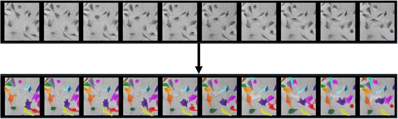
A visual montage of our algorithm’s output is shown in Figure 3a. To benchmark our method, we reserved 10% of our annotated data solely for testing. We also made use of the ISBI cell tracking dataset; where necessary, we used our pipeline to create label movies of these data. As a baseline for the current state-of-the-art, we used an existing implementation of the Viterbi algorithm29,40. One challenge of benchmarking tracking methods is that errors can arise from both segmentation and tracking. Here, we make use of three different tracking metrics. The first are confusion matrices for our deep learning model, which provides a sense of which linkage errors are most likely. The second is a graph-based metric35,41 that treats cell lineage as a directed acyclic graph (DAG). The number of graph operations (split/delete/add a node and delete/add/change an edge) needed to map the DAGs generated by an algorithm to the ground truth DAGs is used to generate a score from 0 to 1. Last, we quantified the true positive, false positive, and false negative rates for detecting cell divisions, one of the most challenging tasks of cell tracking.
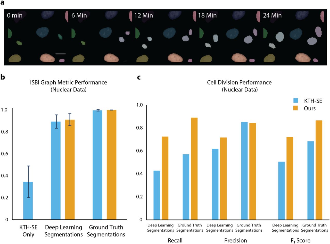
Benchmarking demonstrates that deep learning achieves state-of-the-art performance on cell tracking tasks for a variety of cell types. (a) A montage of tracking results for fluorescent images of cell nuclei and brightfield images of cells. (b) Confusion matrices for our deep learning model identify the linkages between mother cells and daughter cells as our dominant error mode. These linkage errors lead to erroneous and missed divisions. (c) A graph-based metric for cell tracking demonstrates that deep learning enables state-of-the-art performance, with the bulk of this performance boost coming from improved segmentations. (d) Analysis of performance in cell division detection reveals that the performance boost offered by deep learning comes from more accurate detection of cell divisions.
We first computed confusion matrices for our method on our testing dataset; these are shown in the Supplemental Information. These demonstrate that the most common error made by our method is confusing linkages between the same cell with linkages between mother and daughter cells. This leads to false division events, where the mother cell only has one daughter, and missed cell divisions. The former can be mitigated with appropriate post-processing. Next, we used the graph-based metric to compare the performance of our method to a Viterbi based method that has produced state-of-the-art performance in the ISBI cell tracking challenge; this is shown in Figure 3b. To separate cell segmentation performance from cell tracking performance, we applied this metric in three settings. First, we used a classical computer vision method to segment cells and applied the Viterbi cell tracking algorithm to generate a baseline score. Next, to measure the improvement provided by deep learning-enabled cell segmentation, we used deep learning to generate cell segmentations and applied both the Viterbi and our method to link cells together over time. Last, to measure the improvement provided by deep learning-enabled cell tracking, we used our ground truth segmentations as the input to both cell trackers. This comparison (Figure 3b) reveals that the bulk of the performance boost offered by deep learning comes from improved cell segmentations, an insight that is consistent with previous work13. This comparison also shows that our deep learning-enabled cell tracker outperforms the Viterbi algorithm on these data with respect to the graph-based metric, albeit by a small margin.
While the graph-based metric provides a global measure of performance, it is less informative for rare but important events like cell divisions. To complete our analysis, we quantified the recall, precision, and F1 score for cell division detection on our held-out datasets. This was done for both deep learning generated and ground truth segmentations for our method and the Viterbi algorithm. As seen in Figure 3c, deep learning provides a marked improvement in cell division detection, and hence lineage construction. With ground truth segmentations, our approach achieves a recall and precision of 89% and 84%; the Viterbi algorithm achieves 57% and 85% respectively on these measures. The performance of our method falls to a recall of 72% and a precision of 71% when deep learning generated segmentations are used. These results are consistent with the minor differences seen in the graph-based metric because divisions are rare events, and hence require only a few graph operations to fix if they are misidentified. This analysis highlights the strength of our approach; live-cell imaging experiments that require correct lineage construction stand to benefit the most.
Last, because our deep learning model was trained in the same fashion as Siamese neural networks (i.e. same vs different), we wondered whether it would generalize beyond just nuclear data. To test this, we used our crowdsourcing pipeline to generate label movies of brightfield and fluorescent cytoplasmic data from the ISBI cell tracking challenge. We then used the segmentations from these label movies as the input into our cell tracker. Surprisingly, our cell tracker performed markedly well on this challenge, despite never having seen cytoplasmic data. This finding means that single model can be used to track cells irrespective of the imaging modality. This raises the possibility of a pipeline that can process live-cell imaging data while being agnostic to image type or acquisition parameters. As a proof of principle, we constructed a pipeline that uses deep learning models to find the relative scale of input images to our training data and identify the imaging modality. Using this information, we can rescale images, direct them to the appropriate segmentation model, and then send the results to our deep learning-based cell tracker for lineage construction. While this demonstrates the feasibility of analyzing diverse datasets with a single pipeline, additional training data is necessary to produce cytoplasmic segmentations accurate enough for automated analysis.
Discussion
Live-cell imaging is a transformative technology. It has led to numerous insights into the behavior of single cells and will continue to do so for many years to come as imaging and reporter technologies evolve. While the adoption of this method has typically been limited to labs with the computational expertise single cell analysis of these data demands, the arrival of deep learning is changing this landscape. With suitable architectures and deployment tools, deep learning can turn single cell image segmentation into a data annotation problem. With the work we present here, the same can be said for cell tracking. The applications of this technology are numerous, as it enables high throughput studies of cell signaling, cell lineage experiments, and potentially dynamic live-cell imaging-based screens of pharmaceutical compounds.
While deep learning methods are powerful, they are not without limitations. This is particularly true for our approach. Accurate detection is still essential to cell tracking performance, and deep learning-based segmentation methods still make impactful errors as cells become more crowded. We expect this to be mitigated as more expansive sets of data are annotated, and as segmentation methods that use spatiotemporal information to inform segmentation decisions come online42. This method, and all supervised machine learning methods, is limited by the training data that empower it. Our training dataset contains less than 1000 cell divisions; we expect division detection to become more accurate with additional annotated data. Because our training data did not include perturbations that markedly change cell phenotypes or fates (i.e. apoptosis or differentiation), it is possible performance will be limited if these are features of processed data. This can be mitigated by collecting additional training data; we anticipate our existing models combined with a human-in-the-loop approach will enhance future annotation efforts. We also focused on 2D images, as are collected with widefield imaging. Modern confocal and light sheet microscopes can collect 3D data over long time periods. We suspect that our approach can be adapted to these data by using 3D deep learning sub-models, but the requisite annotation task is more challenging than the one undertaken here.
Lastly, our work has centered on live-cell imaging of mammalian cell lines. While these are important model systems for understanding human biology, and the potential of deep learning applications to these systems has for improving human health is substantial, they vastly under sample the diversity of life. Much of our understanding of living systems comes from basic science explorations of bacteria, yeast, and archaea. Live-cell imaging and single cell analysis are powerful methods for these systems; extending deep learning-enabled methods to these systems43 by annotating the requisite data could be just as impactful, if not more so, as the discoveries that will be derived from the work presented here.
Author contributions
EM, WG, and DVV conceived of the project; EM, EB, MS, DB, WG, and DVV designed and wrote the cell tracking algorithm and its deployment; EB, EM, and GM designed and wrote the Caliban software; GM designed and oversaw the data annotation; GM, NK, IC, DK, CP, and TP annotated data; MS, EM, and CP designed and performed benchmarking; TK and EP collected data for annotation; EM and DVV wrote the paper; DVV supervised the project.
Datasets
All of the data used in this paper and the associated annotations can be accessed at http://www.deepcell.org/data or at http://www.github.com/vanvalenlab through the datasets module.
Source code
A persistent deployment of the software described here can be accessed at http://www.deepcell.org. All source code for cell tracking is available in the DeepCell repository at http://www.github.com/vanvalenlab/deepcell-tf. The source code for the Caliban software is available at http://www.github.com/vanvalenlab/Caliban. Detailed instructions are available at http://deepcell.readthedocs.io/.
Competing interests
The authors have filed a provisional patent for the described work; the software described here is available under a modified Apache license and is free for non-commercial uses.
Supplemental Information
Cell line acquisition and culture methods
We used the mammalian cell lines NIH-3T3, HeLa-S3, HEK 293, and RAW 264.7 to collect training data for nuclear segmentation and the cell lines NIH-3T3 and RAW 264.7 to collect training data for augmented microscopy. All cell lines were acquired from ATCC. The cells have not been authenticated and were not tested for mycoplasma contamination.
Mammalian cells were cultured in Dulbecco’s modified Eagle’s medium (DMEM, Invitrogen or Caisson) supplemented with 2mM L-Glutamine (Gibco), 100 U/ml penicillin, 100μg/ml streptomycin (Gibco or Caisson), and either 10% fetal bovine serum (Omega Scientific or Thermo Fisher) for HeLa-S3 cells, or 10% calf serum (Colorado Serum Company) for NIH-3T3 cells. Cells were incubated at 37°C in a humidified 5% CO2 atmosphere. When 70-80% confluent, cells were passaged and seeded onto fibronectin coated glass bottom 96-well plates (Thermo Fisher) at 10,000-20,000 cells/well. The seeded cells were then incubated for 1-2 hours to allow for cell adhesion to the bottom of the well plate before imaging.
Collection of live-cell imaging data
For fluorescent nuclear imaging, mammalian cells were seeded onto fibronectin (Sigma, 10ug/ml) coated glass bottom 96-well plates (Nunc) and allowed to attach overnight. Media was removed and replaced with imaging media (FluoroBrite DMEM (Invitrogen) supplemented with 10mM Hepes, 1% FBS, 2mM L-Glutamine) at least 1 hour prior to imaging. For nuclear imaging, cells without a genetically encoded nuclear marker were incubated with 50ng/ml Hoechst (Sigma) prior to imaging. For cytoplasm imaging, cells were incubated with 2 µM CellTracker CMFDA prior to imaging. Cells were imaged with either a Nikon Ti-E or Nikon Ti2 fluorescence microscope with environmental control (37°C, 5% CO2) and controlled by Micro-Manager or Nikon Elements. Images were acquired with a 20x objective (40x for RAW 264.7 cells) and either an Andor Neo 5.5 CMOS camera with 2×2 binning or a Photometrics Prime 95B CMOS camera with 2×2 binning. All data was scaled to so that pixels had the same physical dimension prior to training. Fluorescence images were taken for nuclear data, while both brightfield and fluorescence images were taken for cytoplasmic data. For time-lapse experiments, images were acquired at 6-minute intervals.
Deep learning architecture for single-cell segmentation
Our pipeline for single cell segmentation is shown in Figure S1. This pipeline uses deep learning models to rescale images and direct them to the appropriate segmentation. We used modified RetinaMask38 models for single cell segmentation of fluorescent nuclear, fluorescent cytoplasm, and brightfield images. RetinaMask generates instance masks in a fashion similar to Mask-RCNN but uses single shot detection like RetinaNet44 rather than feature proposals45 to identify objects. Each model used a ResNet50 backbone pre-trained on ImageNet. For nuclear segmentation, we used the P3 and P4 feature pyramid layers for object detection with an anchor size of 16 and 32 pixels respectively. For the fluorescent cytoplasmic and brightfield segmentation, we used the P3, P4, P5, and P6 layers with anchor sizes of 32, 64, 128, and 256 pixels. For all three models, we attached two semantic segmentation heads46 to predict pixelwise and deep watershed segmentations. This encouraged the backbone and feature pyramid network to learn more general image features. We used a weighted softmax loss for both heads that was weighted by 0.1. All three models were trained on their respective datasets in the same fashion. We used the Adam47 optimization algorithm with a learning rate of 10−5 and clip norm of 0.001, batch size of 4, and L2 regularization strength of 10−5 for 16 epochs on a NVIDIA V100 graphics card. For the nuclear data, we ensured that our training/validation split was the same as was used for training the cell tracking model. Our post processing consisted of removing segmentation masks that have high overlap with >2 other masks. Masks that only overlapped with 1 other mask were resolved using a marker based random walker segmentation step48. All masks smaller than 100 pixels were also removed during post processing. For nuclear segmentation, we used the output of the watershed semantic segmentation mask to add cells that were missed by the RetinaMask object detection.
Deep learning models for scale and image type detection
To develop a live-cell imaging analysis workflow that is agnostic to imaging modality and acquisition parameters, we trained two deep learning models for detecting scale and image type. The scale detection model sought to identify the relative scale of between an input image and our training data; we applied affine transformations to our training data to create images of different scales. The model consisted of a MobileNetV2 backbone connected to an average pooling layer and followed by two dense layers. The model was trained for 20 epochs on a combined dataset (nuclear, fluorescent cytoplasmic, and brightfield images) using a mean squared error (MSE) loss. We used the Adam optimization algorithm with a learning rate of 10−5 and clip norm of 0.001, batch size of 64, and L2 regularization strength of 10−5 on an NVIDIA V100 graphics card. The image type detection model consisted of a MobileNetV2 backbone connected to an average pooling layer followed by two dense layers and a softmax layer. The model was trained for 20 epochs on a combined dataset using a weighted categorical crossentropy loss. We used We used the Adam optimization algorithm with a learning rate of 10−5 and clip norm of 0.001, batch size of 64, and L2 regularization strength of 10−5 on an NVIDIA V100 graphics card. The scale detection model achieved a mean absolute percentage error of 0.85% on validation data while the image type detection achieved a classification accuracy of 98% on validation data. We found that using the MobileNetV2 backbone provided similar performance to larger networks while offering a higher inference speed and lower memory footprint.
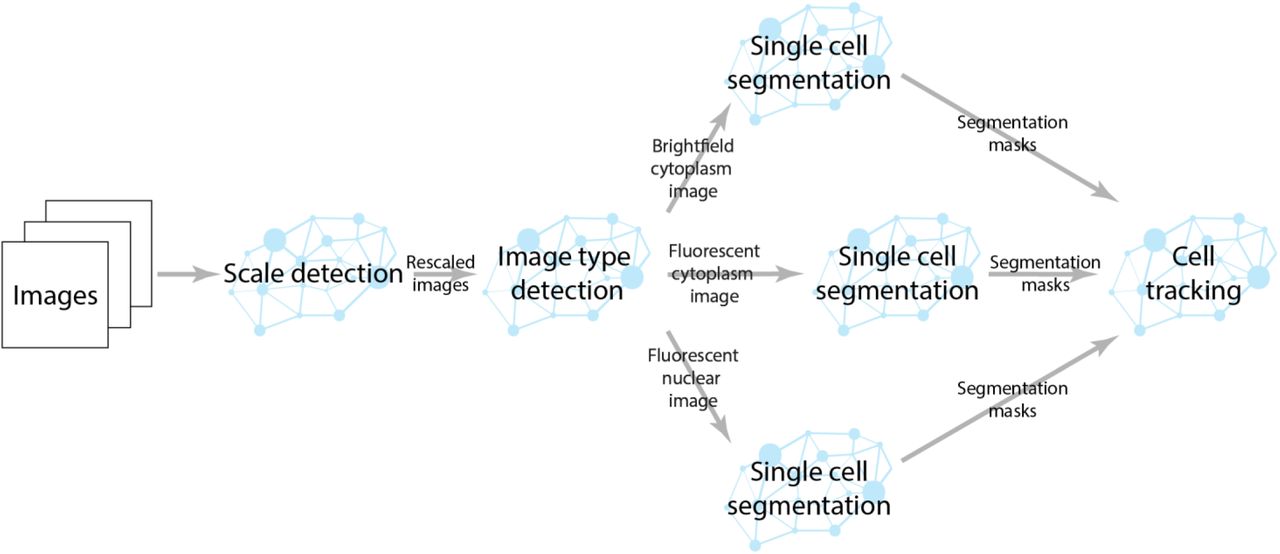
Computational pipeline for single cell segmentation. Our pipeline uses a scale detection deep learning model to rescale input images to the same physical pixel dimensions of our training data. Another deep learning model detects whether the rescaled images are fluorescent nuclear images, fluorescent cytoplasm images, or brightfield images. Once the image type is determined, the images are sent to a RetinaMask based deep learning model for single cell segmentation. The segmentation masks are then sent to the cell tracking deep learning model to construct cell lineages.
Segmentation benchmarking
Because segmentation performance is critical to cell tracking performance, we performed rigorous benchmarking during model optimization. In addition to pixel-based metrics, we also used an object-based approach36 to segmentation benchmarking. This approach compares ground truth and prediction segmentations to identify segmentation errors. Our first step is to link prediction and ground truth segmentations based on object overlap – this can be thought of as constructing of a DeBruijn graph where we are using objects rather than sequences. We solve this problem using a linear assignment framework in a manner akin to how we link cells during cell tracking. We construct a cost matrix where the cost of linking two cells is 1 − iou, where iou is the intersection over union of those two cells. Leaving a ground truth cell unassigned (missed detection) or a prediction cell unassigned (gained detection) has a cost of 0.4. This means for a ground truth and predicted cell to be linked, they must have an iou of at least 0.6.
All the unassigned cells are then gathered for a second round of construction of graph construction to classify error types. This is shown in Figure S2. We view each cell as a node and examine all pairs of unassigned ground truth cells and unassigned predicted cells; we link two cells if they have an iou greater than 0.1. We then extract all the subgraphs of this graph and categorize them into three groups. The first group consists of all subgraphs that have a single node (i.e. the highest degree of any node is 0). If the node is a ground truth cell this corresponds to a missed detection (i.e. a false negative); if the node is a predicted cell this corresponds to a gained detection (i.e. a false positive). The next group consists of all subgraphs where the highest degree node has degree 1. Each subgraph in this group has one node that corresponds to a ground truth cell and one node that corresponds to a prediction cell. Because these cells were not assigned in the first round of graph construction, they correspond to a missed detection and a gained detection. The third group are all subgraphs with a node that has degree > 1. This group can be further divided into three subgroups based on the type and uniqueness of the highest degree node. If the highest degree node is a ground truth cell and is unique, then it corresponds to a splitting error. If the highest degree node is a predicted cell and is unique, it corresponds to a merge error. If the highest degree node is not unique, then it falls into a third class which we call catastrophes. Catastrophe’s involve both splitting and merging mistakes, but it is not possible to decouple the two from the subgraphs. We have found that catastrophes become increasingly common in dense datasets, and that their inclusion was essential to accurately categorize segmentation errors. One limitation of this approach is that it relies on accurate ground truth datasets. We found that segmentation “errors” often reflected errors in training data.

Subgraph classification enables the identification of merge, split, and catastrophe errors in cell segmentations.
The segmentation benchmarks for our segmentation model are given in Tables S1 and S2. For nuclear segmentation, we included feature-nets that were trained in a pixel-wise and deep watershed fashion for comparison. For all benchmarks, we removed objects smaller than 100 pixels from the ground truth and prediction masks prior to benchmarking.

Segmentation benchmarks for deep learning segmentation models for fluorescent nuclear images. The RetinaMask approach provides a mild improvement over pixel-wise and deep watershed approaches to segmentation with feature-nets. This improvement allows for more accurate cell lineage construction. Benchmarking of cytoplasm segmentation models was performed on brightfield images.
Model training and post processing for the cell tracking deep learning model
We used a hybrid convolutional/recurrent deep learning model for identifying whether an existing track of cells and a candidate cell are the same, different, or have a mother daughter relationship. The architecture is described in the main text; source code for the model containing the full implementation is available at http://www.github.com/vanvalenlab/deepcell-tf under the deepcell.model_zoo library. The cell tracking deep learning model was trained using stochastic gradient descent with momentum. We used a batch size of 128, learning rate of 0.01, momentum of 0.9, and learning rate decay of 0.99; the model was trained for 10 epochs, with each epoch consisting of ∼800,000 examples. For post processing, we examined the lineage graphs to identify and remove false division events. A false division event was classified as divisions in a lineage with only one mother-daughter pair and within 9 frames of another division.
Grid search for hyperparameter optimization
Our cell tracking framework contains several hyperparameters including the birth parameter (b), the death parameter (d), division threshold (div), and the number of frames (f) extracted for each track. We performed a grid search to find the optimal values for these hyperparameters. Candidate values for each hyperparameter (b – 0.9, 0.95, 0.99, d – 0.9, 0.95, 0.99, div – 0.9, 0.95, 0.99, f – 3, 5, 7, 9). We performed the grid search in parallel by submitting Jupyter notebooks as Jobs in a Kubernetes cluster. The grid search revealed the optimal values were b = 0.99, d = 0.99, div = 0.9, and f = 7.
Cell tracking benchmarking
In addition to using the ISBI executable to benchmark our cell tracker, we developed a graph-based approach to benchmark cell divisions. This approach treats the ground truth and predicted lineages as a graph, with each cell at each time point being a node. We use the intersection over union to link nodes in the ground truth and predicted graphs as being the same cell. All nodes of degree > 2 were identified as cell division events; using this information, we quantified the number of true positive, false positive, and false negative detections.

Optimization and benchmarking of a deep learning-based cell tracker. (a) A hyperparameter search reveals that a track length of 7 frames provides optimal performance. The most common error type is misclassifying two cells that are the same as having a mother-daughter relationship. (b) Recall and precision for cell division detection on our nuclear data as well as nuclear data from the ISBI cell tracking challenge. We evaluated the performance of a Viterbi based algorithm (KTH) as well as our deep learning approach. (c) ISBI graph metric performance of a Viterbi based algorithm and our deep learning approach on nuclear and cytoplasmic data. The bulk of the performance boost from deep learning is due to more accurate cell detection. Fluorescent cytoplasmic data was not benchmarked due to poor segmentations.
Caliban implementation
A desktop version of Caliban was implemented in Python and can be run from a Docker container. The full source code is available at https://github.com/vanvalenlab/caliban.
Instructions for crowdsourced dataset annotation
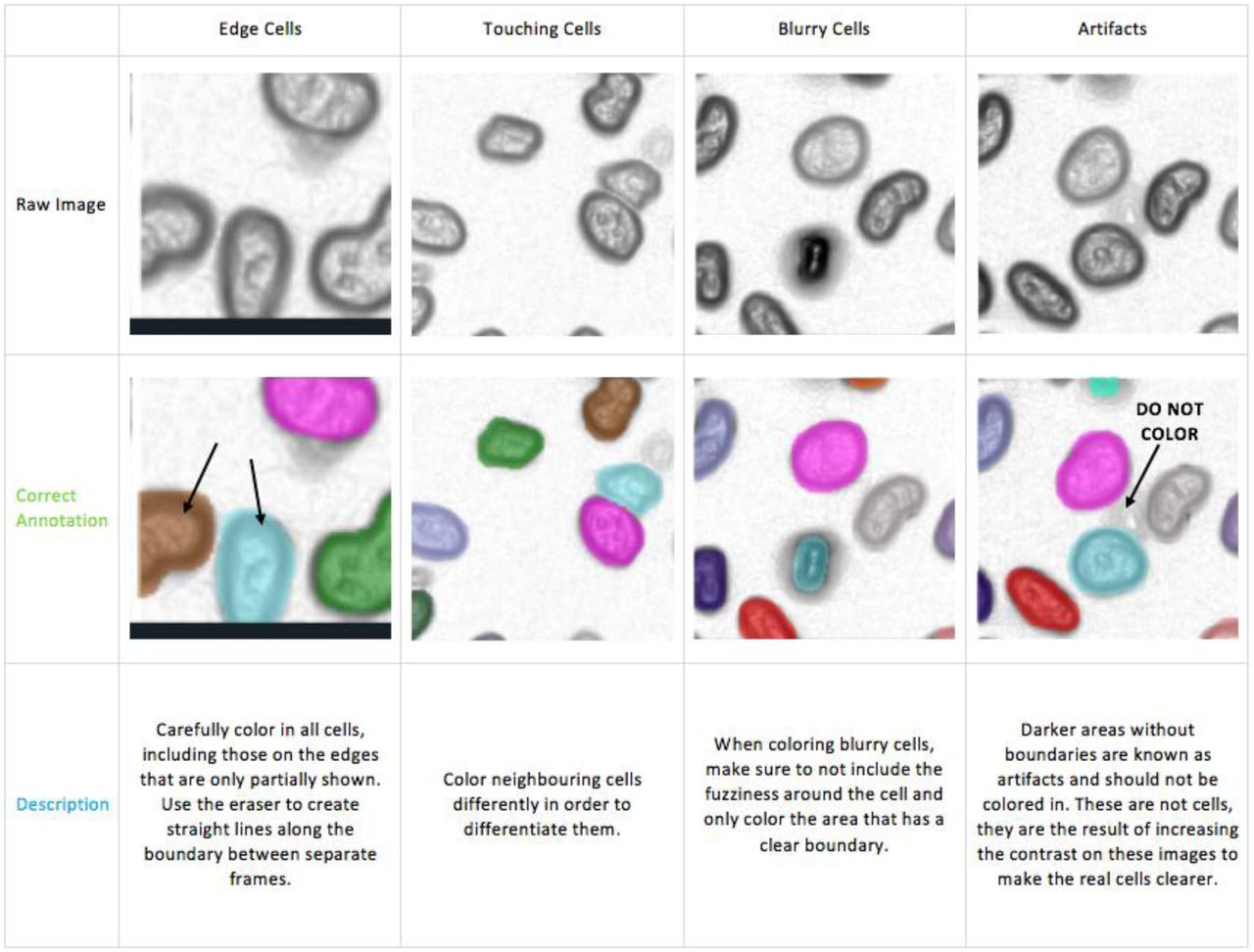
We performed our crowdsourced data annotation on the Figure 8 platform. The instructions given to annotators, which include common error types, are included below. The cost for annotating each dataset was adjusted so that contributors were paid ∼$ 4-5/hour. Ignoring the annual cost of a Figure 8 subscription, we found that the marginal cost of annotating a single cell nucleus was ∼1.5 cents while the marginal cost of annotating a single cell cytoplasm was ∼5.2 cents. Here, we provide the instructions given to the annotators.
Nuclear Time-lapse Cell Annotation
Overview
In this task you will be asked to individually label cells in frames of a microscopy video.
Background
Our group is in the process of writing a computer program to automatically identify and track the movement of individual cells in microscope images. To help us do this, we’re asking you to help create annotated datasets where single cells are manually identified. We can then feed this into the computer program to teach it how to accurately identify cells by itself. The program developed using the data you are annotating will be used in other research laboratories to study a range of topics, including viruses and cancer cells. The software we create is only as good as the data used to create it, so accuracy in your annotations is extremely important.
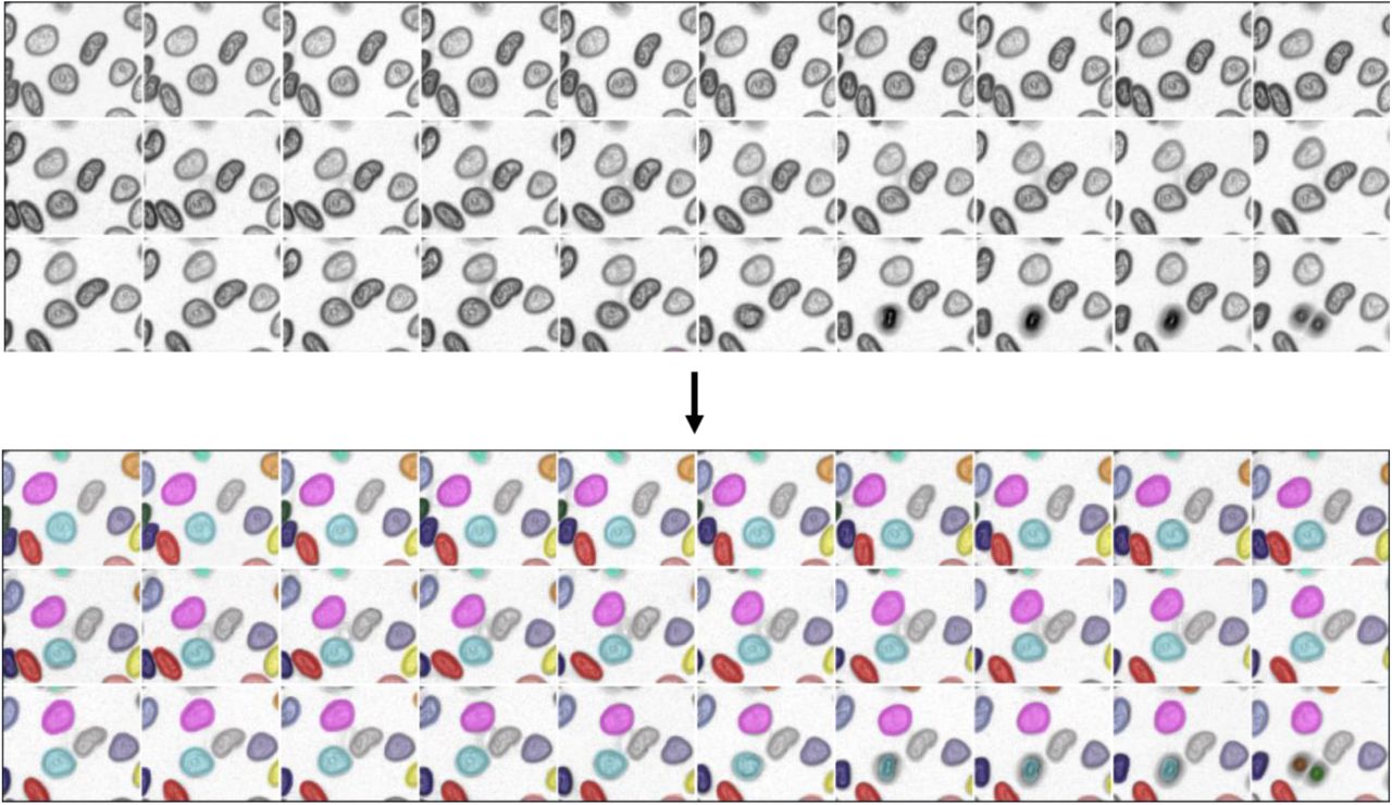
In this job, each image consists of a sequence of snapshots in time, ordered from left to right, top to bottom. Every image in this sequence needs to be annotated. An example of what the image should look like before and after your annotation is shown below:

Annotation Instructions
You must stick to the following rules when labelling cells (further explanations are provided below):

One good strategy to use would be to start from a specific region and follow one cell at a time across all the frames. After the first cell is colored the same across all the frames it is present in, go back and choose a neighboring one. Continue doing this to build up to the entire frame, one cell at a time (never reuse colors for different cells, even if the cell disappears before the end of the frames).
Annotation Technique
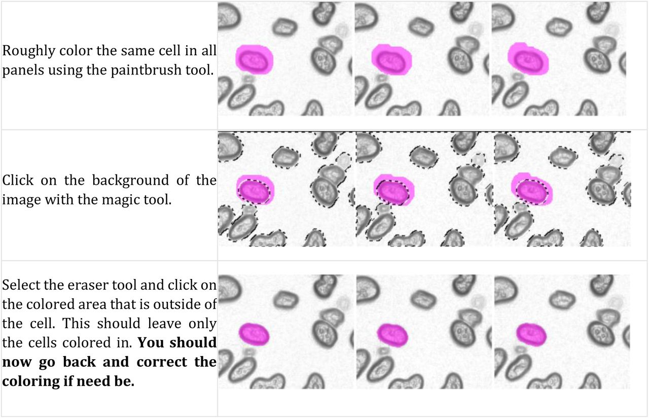
Zoom in on a frame and use the brush tool to outline the cell and fill in the middle, changing the brush size using the slider. Use the eraser tool to correct mistakes.
OR

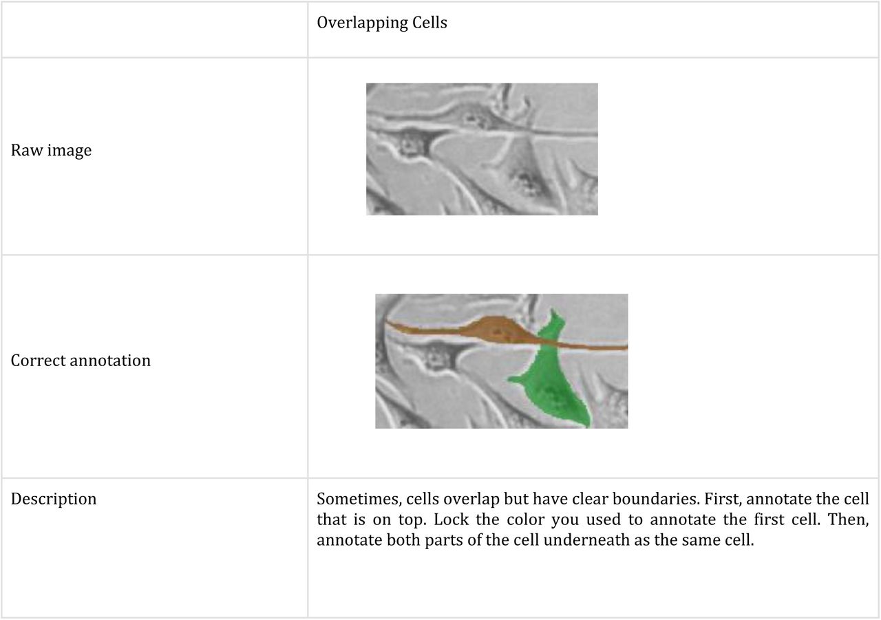
Examples

Video instructions
A video explaining the described labelling process is here: https://youtu.be/tvzGl5b1NDw
Cytoplasm Time-lapse Cell Annotation
Overview
In this task you will be asked to individually label cells in frames of a microscopy video.
Background
Our group is in the process of writing a computer program to automatically identify and track the movement of individual cells in microscope images. To help us do this, we’re asking you to help create annotated datasets where single cells are manually identified. We can then feed this into the computer program to teach it how to accurately identify cells by itself. The program developed using the data you are annotating will be used in other research laboratories to study a range of topics, including viruses and cancer cells. The software we create is only as good as the data used to create it, so accuracy in your annotations is extremely important.
In this job, each image consists of a sequence of snapshots in time, ordered from left to right. Every image in this sequence needs to be annotated. An example of what the image should look like before and after your annotation is shown below:
Annotation Instructions
You must stick to the following rules when labelling cells (further explanations are provided below):

One good strategy to use would be to start from a specific region and follow one cell at a time across all the frames. After the first cell is colored the same across all the frames it is present in, go back and choose a neighboring one. Continue doing this to build up to the entire frame, one cell at a time (never reuse colors, even if the cell disappears before the end of the frames).
Annotation Technique
Zoom in on a frame and use the brush tool to outline the cell and fill in the middle, changing the brush size using the slider. Use the eraser tool to correct mistakes. It is okay if you color in the black edges between images, but NOT if the annotation crosses over into the next image.
Examples


Video instructions
A video explaining the described labelling process is here: https://youtu.be/7nY90iJ1HZY
Acknowledgements
We thank Anima Anandkumar, Michael Angelo, Michael Elowitz, Christopher Frick, Lea Geontoro, Kerwyn Casey Huang, and Gregory Johnson for helpful suggestions and sharing data. We thank Ian Brown and Andy Butkovic for assistance using the Figure 8 image annotation platform, as well as numerous anonymous annotators whose efforts enabled this work. We also thank Henrietta Lacks for graciously donating source material. We gratefully acknowledge support from the Paul Allen Family Foundation through the Discovery Centers at Stanford University and Caltech, The Rosen Center for Bioengineering at Caltech, The Center for Environmental and Microbial Interactions at Caltech, Google Research Cloud, Figure 8’s AI for everyone award, and a subaward from NIH U24CA224309-01.
References


