

Abstract
To correct for a large number of hypothesis tests, most researchers rely on simple multiple testing corrections. Yet, new methodologies of post-selection inference could potentially improve power while retaining statistical guarantees, especially those that enable exploration of test statistics using auxiliary information (covariates) to weight hypothesis tests for association. We explore one such method, adaptive p-value thresholding (Lei & Fithian 2018) (AdaPT), in the framework of genome-wide association studies (GWAS) and gene expression/coexpression studies, with particular emphasis on schizophrenia (SCZ). Selected SCZ GWAS association p-values play the role of the primary data for AdaPT; SNPs are selected because they are gene expression quantitative trait loci (eQTLs). This natural pairing of SNPs and genes allow us to map the following covariate values to these pairs: independent GWAS statistics from genetically-correlated bipolar disorder, the effect size of SNP genotypes on gene expression, and gene-gene coexpression, captured by subnetwork (module) membership. In all 24 covariates per SNP/gene pair were included in the AdaPT analysis using flexible gradient boosted trees. We demonstrate a substantial increase in power to detect SCZ associations and it is especially apparent using gene expression information from the developing human prefontal cortex (Werling et al. 2019), as compared to adult tissue samples from the GTEx Consortium. We interpret these results in light of recent theories about the polygenic nature of SCZ. Importantly, our entire process for identifying enrichment and creating features with independent complementary data sources can be implemented in many different high-throughput settings to ultimately improve power.
Large scale experiments, such as scanning the human genome for variation affecting a phenotype, typically result in a plethora of hypothesis tests. To overcome the multiple testing challenge, one needs corrections to simultaneously limit false positives while maximizing power. Introduced by Benjamini & Hochberg (1995), false discovery rate (FDR) control has become a popular approach to improve power for detecting weak effects by limiting the expected false discovery proportion (FDP) instead of the more classical Family-Wise Error Rate. The Benjamini-Hochberg (BH) procedure was the first method to control FDR at target level α using a step-up procedure that is adaptive to the set of p-values for the hypotheses of interest (Benjamini & Hochberg 1995). Other methods for FDR control have led to improvements in power over BH by incorporating prior information, such as by the use of p-value weights (Genovese et al. 2006). In the “omics” world – genomics, epigenomics, proteomics, and so on – the challenge of multiple testing is burgeoning, in part because our ability to characterize omics features grows continually and in part because of the realization that multiple omics are required for describing phenotypic variation. One might imagine merging complementary omics data and tests using a priori hypothesis weights to improve power; however, until recently, it was not clear how to choose these weights in a data driven manner.
Recent methodologies have been proposed to account for covariates or auxiliary information while maintaining FDR control (Scott et al. 2015, Ignatiadis et al. 2016, Boca & Leek 2018, Li & Barber 2019, Zhang et al. 2019). We implement a selective inference approach, called adaptive p-value thresholding procedure (Lei & Fithian 2018, AdaPT), to fully explore prior auxiliary information while maintaining guaranteed finite-sample FDR control. In a recent review, Korthauer et al. (2019) compared the performance of AdaPT with other covariate-informed methods for FDR control in simple one and two-dimensional covariate examples. One of the weaknesses they ascribe to AdaPT is the unintuitive modeling framework for incorporating covariates; however, we fully embrace AdaPT’s flexibility via gradient boosted trees in a much richer, high-dimensional setting. Our boosting implementation of AdaPT easily scales with more covariates, enabling practitioners to capture interactions and non-linear effects from the rich resources of prior information available. In this manuscript, we demonstrate our gradient boosted trees implementation of AdaPT on results from genome-wide association studies (GWAS), incorporating covariates constructed from independent GWAS and gene expression studies. Specifically, we apply AdaPT to GWAS for detecting single nucleotide polymorphisms (SNPs) associated with schizophrenia (SCZ) using bipolar disorder (BD) GWAS results from an independent sample as a covariate. Additionally, we incorporate results from the recent BrainVar study to identify a set of expression-SNPs (eSNPs) based on 176 neurotypical brains, sampled from pre-and post-natal tissue from the human dorsolateral prefrontal cortex (Werling et al. 2019). Along with the genetically correlated BD z-statistics, we create additional features from this complementary data source by summarizing the associated developmental gene expression quantitative trait loci (eQTL) slopes and membership in gene coexpression networks. We demonstrate that this process of identifying an enriched set of eSNPs and applying AdaPT with covariates summarizing gene expression from the developing human prefrontal cortex yields substantial improvement over the same pipeline of analysis applied to adult tissue samples from the GTEx Consortium (2015). Furthermore, we see improvements in the discovery rate with each additional piece of information from the BrainVar study and validate the replication of our results using more recent, independent SCZ studies.
This study had two goals, to explore the use of AdaPT in a realistic high-dimensional multiomics setting and to determine what can be learned about the neurobiology of SCZ by this exploration. Our results revealed the power of incorporating auxiliary information with flexible gradient boosted trees. While each covariate independently provided at best a modest increase in power, our adaptive search discovered a more complex model with far greater power. These discoveries also led to greater support for the polygenic basis of SCZ, complementing recent findings, suggesting that there are many physiological avenues to its underlying neurobiology. We emphasize that the process and analysis undertaken with this implementation of AdaPT can be extended to a variety of “omics” and other settings to utilize the rich contextual information that is often ignored by standard multiple testing corrections. We highlight this feature by analyzing two other sets of GWAS studies, type 2 diabetes (T2D) and body mass index (BMI), using results from these analyses to interpret findings from SCZ.
Results
Methodology overview
AdaPT is an iterative search procedure, introduced by Lei & Fithian (2018), for determining a set of discoveries/rejections, ℛ, with guaranteed finite-sample FDR control at target level α under conditions outlined below. We apply AdaPT to the prepared collection of p-values and auxiliary information, (pi, xi)i∈n, testing hypothesis Hi regarding SNP i ‘s association with the phenotype of interest (e.g. SCZ). The covariates from some feature space, xi ∈𝒳, capture information collected independently of pi, but potentially related to whether or not the null hypothesis for Hi is true and the effect size under the alternative. AdaPT provides a flexible framework to incrementally learn these relationships, potentially increasing the power of the testing procedure, while maintaining valid FDR control.
For each step t = 0, 1, … in the AdaPT search, we first determine the rejection set ℛt = {i: pi ≤ st(xi)}, where st(xi) is the rejection threshold at step t that is adaptive to the covariates xi. This provides us with both the number of discoveries/rejections Rt = |ℛt|, as well as a pseudo-estimate for the number of false discoveries At = |{i: pi ≥ 1 - st(xi)}| (i.e. number of p-values above the “mirror estimator” of st(xi)). These quantities are used to estimate the FDP at the current step t,

If  , then the AdaPT search ends and the set of discoveries ℛt is returned. Otherwise, we proceed to update the rejection threshold while satisfying two protocols:
1. updated threshold must be more stringent, st+1(xi) ≤ st(xi), ∀xi ∈𝒳,
2. small and large p-values determining Rt and At are partially masked,

Under these protocols, the rejection threshold can be updated using Rt, At, and  . The flexibility in how this update takes place is one of AdaPT’s key strengths and allows it to easily incorporate other approaches from the multiple testing literature, such as a conditional version of the classical two-groups model (Efron et al. 2001, Scott et al. 2015) with estimates for the probability of being non-null, π1, and the effect size under the alternative, µ.
The algorithm proceeds by sequentially updating the threshold st+1(xi) to discard the most likely null element in the current rejection region, as measured by the conditional local false discovery rate (fdr): i.e.,  is removed from ℛt. With the threshold updated, the AdaPT search repeats by estimating FDP and updating the rejection threshold until the target FDR level is reached
  .
.
This procedure guarantees finite-sample FDR control under independence of the null p-values and as long as the null distribution of p-values is mirror conservative, i.e. the large “mirror” counterparts 1 - pi ≥ 0.5 are at least as likely as the small p-values pi ≤ 0.5. To address the assumption of independence, we select a subset of weakly correlated SNPs detailed in Data, and additionally provide simulations in SI Appendix (Figures S18-S20) showing that AdaPT appears to maintain FDR control in positive dependence settings. However, one practical limitation we encounter with the FDP estimate in Equation 1 is observing p-values exactly equal to one. While this can understandably occur with publicly available GWAS summary statistics, p-values equal to one will always contribute to the estimated number of false discoveries At. This nuance can lead to a failure of obtaining discoveries at a desired target α, such as the reported AdaPT results by Korthauer et al. (2019) for multiple case-studies. However, we demonstrate in SI Appendix an adjustment to the p-values for T2D and BMI GWAS applications which alleviates this problem (Figures S10 and S13), but future work can explore modifications to the FDP estimator itself.
For the modeling step of AdaPT, which estimates conditional local fdr, we use gradient boosted trees, which constructs a flexible predictive function as a weighted sum of many simple trees, fit using a gradient descent procedure that minimizes a specified objective function. In our case, the two objective functions considered correspond to estimating the probability of a test being non-null and the distribution of the effect size for non-null tests. The advantage of this approach to function fitting is that it is invariant to monotonic variable transformations, automatically incorporates important variable interactions, and is able to handle a large number of potentially useful covariates without degrading significantly in performance due to the high dimensionality. In contrast, less effective methods might fail to capture useful information because the covariates are incorrectly scaled for a linear function, because the important information is only revealed through a combination of covariates or because the important signal is simply swamped by the number of possible predictors to search through. Our choice of method gives the flexibility to include many potentially useful covariates without being overly concerned about the functional form with which they enter or their marginal utility. In our implementation, we employ the XGBoost library (Chen & Guestrin 2016) to capitalize on its computational advantages.
Figure 1 displays the full pipeline of our implementation of AdaPT to GWAS summary statistics for SNPs using expression quantitative trait loci (eQTL) to choose the SNPs under investigation. Methods detail the EM algorithm used to model the conditional local false discovery rate with gradient boosted trees.

Summary of AdaPT implementation on GWAS results for selected set of SNPs.
Data
Our investigation includes AdaPT analyses of published GWAS p-values, {pi, i = 1, … n}, for body mass index (Locke et al. 2015, BMI), type 2 diabetes (Mahajan et al. 2018, T2D), and schizophrenia (Ruderfer et al. 2014, SCZ), but we focus our presentation on SCZ results. SCZ is a highly heritable, severe neuropsychiatric disorder. It is most strongly correlated, genetically, with another severe disorder, bipolar disorder (BD) (Lichtenstein et al. 2009, Cross-Disorder Group of the Psychiatric Genomics Consortium 2013). Because of this genetic correlation, reported z-statistics from BD GWAS,  , can be used as informative covariates for determining the SCZ rejection threshold. We use the GWAS summary statistics reported by Ruderfer et al. (2014) available from the Psychiatric Genomics Consortium (PGC), with independent controls for BD and SCZ, as an application of our AdaPT implementation (combined 19,779 SCZ and BD cases with 19,423 controls). Results from more recent studies in Ruderfer et al. (2018) are used for replication analysis of our results (combined 53,555 SCZ and BD cases with 54,065 controls). However, the 2014-only studies from Ruderfer et al. (2014) are a subset of the all-2018 studies from Ruderfer et al. (2018). Although we do not have access to the raw genotype data, we use the fact that both papers report inverse variance-weighted fixed effects meta-analysis results (Willer et al. 2010). We then separate the summary statistics for the 2018-only studies exclusive to Ruderfer et al. (2018), thus independent of the 2014-only studies and an appropriate hold-out to use for replication analysis.
After matching alleles from both 2014-only and all 2018 studies and limiting SNPs to those with imputation score INFO > 0.6 for both BD and SCZ in 2014-only (Ruderfer et al. (2014)), we obtained 1,109,226 SNPs. Rather than test all SNPs, we chose to investigate a selected subset of SNPs, eSNPs, whose genotypes are correlated with gene expression; this additional filtering step captures a set of SNPs that are more likely to be functional and not highly correlated mutually (Nicolae et al. 2010). These eSNPs were identified from two sources. First, we evaluated the Genotype-Tissue Expression (GTEx) V7 project dataset (GTEx Consortium 2015) with adult samples from fifty-three tissues. As the first winnowing step, we identified the set of GTEx eQTLs for any of the available tissues at target FDR level α = 0.05. Rather than use all GTEx eQTLs, however, we winnowed the eQTLs by selecting SNPs whose genotypes are most predictive of expression for each gene. These SNP-gene pairs yielded nGTEx = 31,558 eSNPs.
The second source was the BrainVar study of dorsolateral prefrontal cortex samples across a developmental span (Werling et al. 2019). BrainVar included cortical tissue from 176 individuals falling into two developmental periods: pre-natal, 112 individuals; and post-natal, 60 individuals. We identified nBrainVar = 25,076 eSNPs as any eQTL SNP-gene pairs provided by Werling et al. (2019) meeting Benjamini-Hochberg α ≤ 0.05 for at least one of the three sample sets (pre-natal, post-, and complete = all), resulting in a set of eSNPs of comparable size to the GTEx eSNPs. (Because of the source of the BrainVar eSNPs, we did not analyze these for either BMI or T2D.)
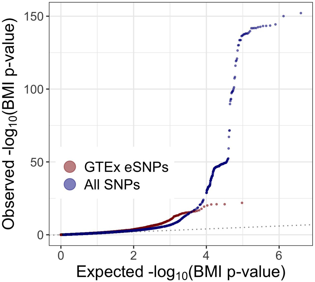
There are only 3,382 SNPs in the intersection set of the two considered definitions for SCZ eSNPs, approximately 10% and 13% of GTEx and BrainVar eSNPs respectively. This relatively minor overlap is likely driven by the temporal difference in when samples are taken for GTEx (adults) as compared to BrainVar (developmental). Figure 2 displays a comparison of SCZ enrichment for the full set of SNPs to both the nGTEx and nBrainVar eSNPs. The BrainVar eSNPs appear to display the highest level of SCZ enrichment and are the primary focus of this manuscript.

A comparison of qq-plots revealing SCZ enrichment for both BrainVar and GTEx eSNPs compared to the full set of SNPs from 2014 studies.
For each eSNP i, we created a vector of covariates xi to incorporate auxiliary information collected independently of pi, including p-values from GWAS studies of related phenotypes, and relationships inferred from gene expression studies. First, we utilize the mapping of eSNPs to genes derived from eQTLs assessed in a relevant tissue type r. Let  denote the set of cis-eQTL genes associated with eSNP i and summarize the level of expression as the average absolute eQTL slope for variants in
  to obtain
  . Additionally, we account for gene co-expression networks as covariates using the J modules generated with weighted gene co-expression network analysis (Zhang & Horvath 2005, WGCNA). For each of the j = 1, …, J WGCNA modules we create an indicator variable
  denoting whether or not eSNP i has any associated cis-eQTL genes in module j.
For the nBrainVar eSNPs, we calculate  where type ∈ {pre, post, complete} to capture the eSNP’s overall expression association across three different points in the developmental span. Additionally, we use the J = 20 WGCNA modules (including unassigned gray) reported by Werling et al. (2019) to create indicator variables
  for j = 1, …, 20. This culminates in a vector of twenty-four covariates
  .
.
For a parallel analysis we create a vector of covariate information  for the nGTEx eSNPs, calculating
  for r ∈ {GTEx cortical tissues} as well as indicator variables for WGCNA modules generated using GTEx cortical tissue samples. A full description of the variables considered for the set of GTEx eSNPs, along with T2D and BMI, is in SI Appendix.
AdaPT discoveries
We proceed to apply the AdaPT search algorithm to the SCZ p-values from the 2014-only studies to both types of eSNPs with their respective vector of covariates,  and
and  , capturing the correlation between BD and SCZ along with gene expression association and network summaries. At target FDR level α = 0.05, AdaPT returns RGTEx = 23 and RBrainVar = 843 discoveries for both the nGTEx = 31,558 and nBrainVar = 25,076 eSNPs respectively. As a baseline, we compare these results to an intercept-only version of AdaPT, which ignores covariates and was found to display a favorable performance in Korthauer et al. (2019). For the GTEx intercept-only results, 91 discoveries were returned versus 361 BrainVar intercept-only discoveries at α = 0.05. The Manhattan plots in Figures 3(A) and (B) compare the discovered BrainVar eSNPs from the intercept-only results to the fully informed AdaPT SCZ results with all twenty-four variables. The stark contrast between the expression data sources further reinforces the association between the SCZ GWAS results and gene expression in developmental periods measured in BrainVar, as compared to adult samples from GTEx. We examine the BrainVar results more closely for the remainder of the manuscript (see Figures S9 and S12 for T2D and BMI eSNP enrichment).

Manhattan plots of SCZ AdaPT discoveries using (A) intercept-only model compared to (B) covariate informed model at target α = 0.05. (C) Comparison of the number of discoveries at target α = 0.05 for AdaPT with varying levels of covariates and (D) their resulting discovery intersections.
Although we focus on the discoveries using the twenty-four covariates described earlier in  , for reference we additionally view the improvement in AdaPT’s performance on the BrainVar eSNPs by incrementally including more eSNP-level covariates. We start with the BD z-statistics:
BD z-stats:
 ,
,BD z-stats + eQTL slopes:
,BD z-stats + eQTL slopes + WGCNA:
.


For each of set of covariates we tune the gradient boosted models (see SI Appendix and Table S1 for details on boosting parameters). Figure 3(C-D) displays the comparison in the number of discoveries between the different sets of covariates at target FDR level α = 0.05. The result yielding the highest number of discoveries is with all twenty-four covariates. For comparison, the results from only using the WGCNA modules,  , are also displayed to show that the substantial improvement in performance results from using all three types of information together rather than from the impact of the WGCNA module indicators independently.
Variable importance and relationships
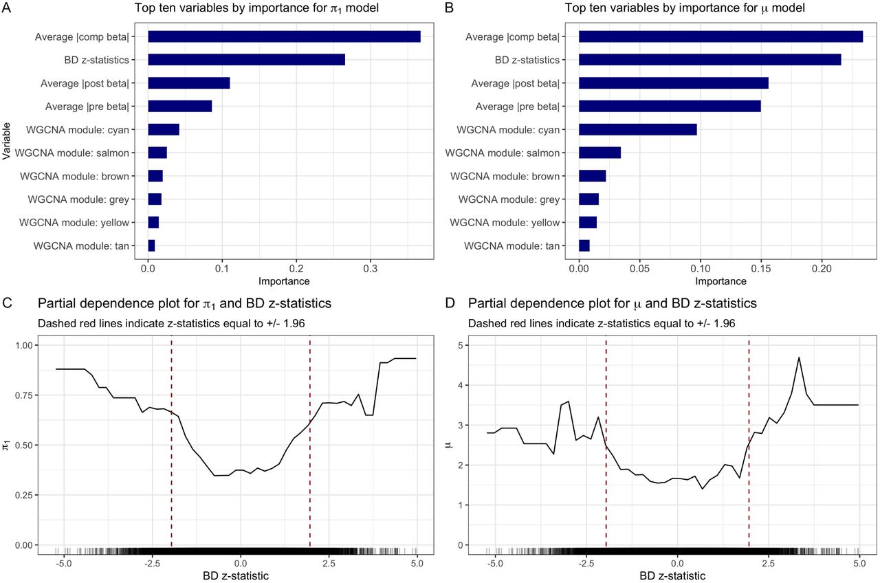
We examine the variable importance and partial dependence plots from the final gradient boosted models returned by AdaPT to provide us with insight into the relationships between each of the covariates considered and SCZ associations. Figures 4(A-B) display the variable importance plots for both the probability of being non-null (π1) and effect size under alternative (µ) models respectively, displaying the relative contribution of each variable based on the total gain from its splits in the gradient boosted trees. We see similarities between both summaries, with the BD z-statistics appearing to be the most important.

Variable importance plots for final AdaPT (A) probability of non-null and (B) effect size under alternative models. (C) Partial dependence plot for probability of being non-null and BD z-statistics. (D) SCZ enrichment of BrainVar eSNPs based on salmon WGCNA module membership.
Figure 4(C) displays the partial-dependence plot (Friedman 2001) for the estimated marginal relationship between the BD z-statistics and the probability of being non-null. This reveals an increasing likelihood for non-null results as the BD z-statistics grow in magnitude from zero, with noticeably sharp increases indicated by the dashed red lines around the nominal thresholds corresponding to BD p-values of 0.05. Figure 4(D) displays the clear enrichment for eSNPs with cis-eQTL genes that are members of the salmon WGCNA module reported by Werling et al. (2019), which also displayed relatively high variable importance. The unassigned gray module also displayed higher variable importance, however, this variable is predictive of SNPs that are classified as null, rather than associated with the phenotype. See SI Appendix for more partial dependence and WGCNA module enrichment plots (Figures S1-S3 for additional SCZ BrainVar results, and Figure S4 for SCZ GTEx).
Replication in independent studies
Next, we examine the replicability of the 2014-only SCZ BrainVar AdaPT results, using  , by checking the nominal discovery replication of the SCZ p-values from the independent 2018-only studies. For simplicity, we consider an AdaPT discovery at target FDR level α = 0.05 to be a nominal replication if its corresponding p-value for the 2018-only studies is less than 0.05. Of the 843 discoveries from the 2014-only studies, approximately 55.2% (465 eSNPs) were nominal replications in the 2018-only studies.
This nominal replication rate is unsurprising given the “winner’s curse” phenomenon, as described in Lohmueller et al. (2003), and does not imply that the rejected hypotheses are actually null. To empirically evaluate this result, we use the final non-null effect size model estimated by the AdaPT search to generate simulated p-values psim using the observed 2018-only studies’ standard errors. We repeatedly generate the simulated p-values one-thousand times for the 843 2014-only discoveries, and calculate the nominal replication rate with psim. The nominal replication rate for the one-thousand simulations ranges from 51% to 64%, with an average of ∼ 57.2%, which provides reassurance regarding the observed rate. More details regarding the simulation process are provided in SI Appendix. Additionally, Figure 5 also displays the relationship between the 2018-only p-values and the resulting 2014-only q-values (Storey 2002) from the AdaPT search on the -log10 scale (see Lei & Fithian (2018) for derivation of AdaPT q-values). The black line represents the increasing smoothing spline relationship between the two, with noticeably increasing evidence indicated by the 2018-only p-values for the set of AdaPT discoveries at α = 0.05.

Black line displays smooth relationship between SCZ p-values from 2018-only studies and the AdaPT q-values from the 2014-only studies. Blue-shaded region indicates AdaPT discoveries at α = 0.05 that are nominal replications, p-values from 2018-only studies < .05 while red region denotes discoveries which failed to replicate.
Gene ontology comparison
With SNP discoveries spanning the genome, including nearly every chromosome, we sought biological insights. We applied gene ontology enrichment analysis (Ashburner et al. 2000, The Gene Ontology Consortium 2018) to the 136 genes obtained from the eQTL variant-gene pairs associated with the 843 discoveries. This analysis produced no clear signal, yielding only a minor enrichment for biological processes related to peptide antigen assembly. Several explanations are plausible, we explore two: either AdaPT is discovering SNPs of such small effect that the discoveries are not meaningful or SCZ is a highly complex disorder with a large number of biological processes involved. For comparison we applied our full pipeline to GWAS summary statistics for T2D (Mahajan et al. 2018). This comparison is of interest because T2D is a disease with a well understood functional basis, and this is a well powered study with a sample size of 898,130 individuals (74,124 T2D cases and 824,006 controls). We restricted our analysis to 176,246 eSNPs based on eQTLs obtained using GTEx data. Next, we created eQTL-based covariates using pancreas, liver, and adipose tissue samples (see SI Appendix and Figures S9-S11 for more details on the implementation). After creating a vector of covariates from GTEx, AdaPT returned 14,920 eSNPs at α = 0.05, resulting in 5,970 associated genes. Applying gene ontology enrichment analysis to this gene list, we discovered enrichment for biological processes related to lipid metabolic process (see Figure 6), consistent with previous literature (Cirillo et al. 2018). These results provide some reassurance that the lack of specificity in the SCZ results can be attributed to the complex etiology of SCZ. For comparison to the well powered BMI GWAS (339,224 subjects), we found a lack of gene ontology enrichment in our gene discoveries, which are detailed in SI Appendix).

T2D gene ontology enrichment analysis results for top ten biological processes based on positive fold enrichment.
Pipeline results for all 2018 studies
In addition to applying the pipeline to SCZ p-values from the 2014-only studies in Ruderfer et al. (2014), we also modeled p-values from all 2018 studies. The latter yields far more discoveries due to smaller standard errors from increased study sizes, even though the covariates were the same: for  , we find 2,228 discoveries at target FDR level α = 0.05 when the pipeline was applied to the p-values for most up-to-date set of studies versus 843 for the 2014-only studies. Notably, the intercept-only version of AdaPT returned 1,865 discoveries at α = 0.05, meaning the covariates contributed to ∼ 19% increase in discovery rate for all 2018 studies versus the ∼ 134% increase (361 to 843 eSNPs) from using the covariates for the 2014-only studies (see Figures S5 and S6). This reinforces the value of using auxiliary information in studies with lower power. Complementary to this observation, AdaPT applied to BMI GWAS yielded more discoveries for the intercept-only version than covariate informed models (details presented in SI Appendix, see Figures S14-S15). Simply accounting for more auxiliary information does not guarantee an improvement in power and the advantages thereof diminishes as power increases, as witnessed by results for all 2018 studies for SCZ and the large-scale BMI GWAS. Additionally, the larger number of discoveries for the SCZ all 2018 studies, 2,228, maps onto 382 genes. Despite this increase, these genes did not reveal any clear signal from the Gene Ontology enrichment analysis, comporting with results from the 2014-only results.
Discussion
Our goals in this study were to explore the use of AdaPT for high-dimensional multi-omics settings and investigate the neurobiology of SCZ in the process. AdaPT was used to analyze a selected set of GWAS summary statistics for SNPs, together with numerous covariates. Specifically, SNPs were selected if they were documented to affect gene expression; these SNP-gene pairs were dubbed eSNPs. Covariates for these eSNPs included independent GWAS test statistics from a genetically correlated phenotype, BD, which were mapped to eSNPs through SNP identity; as well as features of gene expression and co-expression networks, which were mapped to eSNPs through genes. By coupling flexible gradient boosted trees with the AdaPT procedure, relationships among eSNP GWAS test statistics and covariates were uncovered and more SNPs were found to be associated with SCZ, while maintaining guaranteed finite-sample FDR control. The tree-based handling of covariates addresses a perceived weakness of AdaPT, namely the unintuitive modeling framework for incorporating covariates (Korthauer et al. 2019). The pipeline we built should be simple to mimic for a wide variety of omics and other analyses.
Regarding the neurobiology of SCZ, two important findings emerge. First, by comparing results from SCZ GWAS when the expression/coexpression covariates were derived from developing human prefrontal cortex versus those from adult tissue samples from GTEx, the former yielded notably better results. This comports with the development of SCZ itself: first break episodes of psychosis typically occur by early adulthood, somewhat later for women than for men. Furthermore, the results underscore the fact that we can learn more from genetic associations about the neurobiology of SCZ by studying a large-scale developmental series of brains than we can by studying adult tissue; regrettably, however, most brain tissue is obtained from adults, often relatively old adults.
A second point of interest regards the level of complexity underlying the neurobiology of SCZ. If the origins of SCZ arose by perturbations of one or a few pathways, we would expect to converge on those pathways as we accrue more and more genetic associations. On the other hand, if the ways to generate vulnerability to SCZ were myriad — even if there is an single ultimate cause shared across all cases — then we might expect no such convergence, at least with regards to the common variation assessed through GWAS. Gene ontology analysis of associated discovery genes from either the 2014-only or all 2018 studies reveals no enrichment for biological processes for SCZ. There are many possible explanations for these null findings, one of which is simply a lack of power or specificity of our results. However, the result stands in stark contrast to the results for T2D, for which the gene ontology analysis converges nicely on accepted pathways to T2D risk; yet they comport with those for BMI, which is known to have myriad genetic and environmental origins. Therefore our results are consistent with myriad pathways to vulnerability for SCZ, although it is impossible to rule out other explanations: for example, the possibility that we understand so little about brain functions that gene ontology analyses lack specificity. In any case, our results are consistent with two recent theories underlying the genetics of SCZ, namely extreme polygenicity (O’Connor et al. 2019) and “omnigenic” origins (Boyle et al. 2017).
Although the examples considered in this manuscript pertain to omics data, this process can be adapted for a large variety of settings. We demonstrate in SI Appendix (Figures S18-S20) simulations showing that AdaPT appears to maintain FDR control in positive dependence settings emulating linkage disequilibrium (LD) block structure underlying GWAS results. There is a clear need, however, for future work to explore AdaPT’s properties and computational challenges under various dependence regimes. More insight can help determine its appropriateness for improving power versus other approaches, such as those with known structural constraints (Lei et al. 2017). The growing abundance of contextual information available in “omics” settings provides ample opportunity to improve power for detecting associations, using a flexible approach such as AdaPT, when addressing the multiple testing challenge.
Methods
Two-groups model
The most critical step in the AdaPT algorithm involves updating the rejection threshold st(xi). Lei & Fithian (2018) use a conditional version of the classical two-groups model (Efron et al. 2001) yielding the conditional mixture density,
 where the null p-values are modeled as uniform (f0(p|x) ≡ 1). They proceed to use a conservative estimate for the conditional local false discovery rate,
  , by setting 1 - π1(x) = f (1|x).
We model the non-null p-value density with a beta distribution density parametrized by µi,
 where µi = 𝔼 [-log(pi)], resulting in a conditional density for a beta mixture model,

In this form, we can model the non-null probability π1(xi) = 𝔼[Hi|xi] and the effect size for non-null hypotheses µ(xi) = 𝔼[-log(pi)|xi, Hi = 1] with two separate gradient boosted tree-based models. The XGBoost library (Chen & Guestrin 2016) provides logistic and Gamma regression implementations which we use for π1(xi) and µ(xi) respectively.
There are two categories of missing values in these regression problems: Hi is never observed, and at each step t of the search, the p-values for tests {i: pi ≤ st(xi) or pi ≥ 1 - st(xi)} are masked as  . Naturally, an expectation-maximization (EM) algorithm can be used to estimate both
  and
and  by maximizing the partially observed likelihood. The complete log-likelihood for the conditional two-groups model is,

During the E-step of the d = 0, 1, … iteration of the EM algorithm, conditional on the partially observed data fixed at step t,  , we compute both,

 where
where  indicates how likely
  equals pi for non-null hypotheses. The explicit calculations of
  and
and  for both the revealed,
  , and masked p-values,
  , are available in the supplementary materials of (Lei & Fithian 2018).
The M-step consists of estimating  and
and  with separate gradient boosted trees, using pseudo-datasets to handle the partially masked data. In order to fit the model for π1(xi), we construct the response vector
  and use weights
  . Then we estimate
  using the first n predictions from a classification model using
  as the response variable with the covariate matrix (xi)i∈[n] replicated twice and weights
  . Similarly, for estimating
  we construct a response vector
  with weights
  , and again take the first n predicted values using the duplicated covariate matrix.
The conditional local fdr is estimated for each  ,
,
 and we follow the procedure detailed in Section 4.3 of Lei & Fithian (2018) to update the rejection threshold to st+1(xi) by removing test
  from ℛt. A summary diagram of the EM algorithm is displayed in Figure 7.

Summary of AdaPT EM algorithm.
AdaPT gradient boosted trees with CV steps
As a flexible approach for modeling the conditional local fdr, we use gradient boosted trees (Friedman 2001) via the open-source XGBoost implementation (Chen & Guestrin 2016). Gradient boosted trees are an ensemble of many “weak” learners with contributions for making predictions. Let ℱ be the space of functions containing regressions trees, then the sum-of-trees model can be written as,
 where each fp ∈ℱ is an individual tree and we aim to minimize the objective function,
 where L is the loss function and Ω measures the complexity of each tree such as the maximum depth, regularization, etc. Chen & Guestrin (2016) detail the algorithms for fitting the model in an additive manner as well as determining the splits for each tree.
In order to tune the variety of parameters for gradient boosted trees within AdaPT, such as the number of trees P and maximum depth of each tree, we use the cross-validation (CV) approach recommended in Lei & Fithian (2018). If we are considering M different options of boosting parameters, then we evaluate each of the M choices during the modeling phase of the AdaPT search. At step t, we divide the data into K folds preserving the relative proportions of masked and unmasked hypotheses. Then for each set of boosting parameters m = 1, …, M:
For each fold k = 1, …K:
apply EM-algorithm from Figure 7 to estimate
and using parameters m with data from folds {1, …, K}\{k},compute expected-loglikelihood
on hold-out set k using two-groups model parameters from m following convergence,
then compute total across hold-out folds:
.


Finally we use the set of parameters  in another instance of the EM algorithm to estimate
  and
and  on all data.
Computational aspects of AdaPT
Practical decisions are necessary to implement the AdaPT search. In addition to the covariates and p-values (xi, pt,i)i∈[n], an initial rejection threshold s0(xi) is required to begin the search. Rather begin the search with a high starting threshold, such as  recommended by Lei & Fithian (2018), we instead begin the AdaPT search with
  . Our decision to lower the starting threshold is advantageous for multiple reasons. First, intuitively, this starts our search in the regime of interest for target level α = 0.05, where we would not expect to detect discoveries with larger p-values using this flexible multiple testing correction. Additionally, by lowering the starting threshold, more true information is available to the gradient boosted trees at the start of the AdaPT search. For instance, with the set of BrainVar eSNPs, 21,248 true p-values are immediately revealed with
  as compared to only 2,290 when
  . Simulations detailed in SI Appendix show that on average our choice for using a lower threshold results in higher power (Figure S16).
The most computationally intensive part of the procedure is updating the rejection threshold via the EM algorithm. Instead of updating the model for estimating fdrt,i at each step of the search, we re-estimate every [n/20] steps as recommended by Lei & Fithian (2018). However, the inclusion of the previously described K-fold CV procedure (we use K = 5) for tuning the gradient boosted trees obviously adds computational complexity to the AdaPT search, and would be expensive to apply every time the model fitting takes place. Rather, we apply the CV step once at the beginning, and then another time half-way through the search based on the similarity of simulation performance with varying number of CV steps in SI Appendix (Figure S17). Additionally, one needs to choose the potential M model parameter choices. Technically, unique combinations can be used for both models, π1 and µ, but for simplicity we only consider matching settings for both models, i.e. both models have the same number of trees and maximum depth (see SI Appendix and Tables S1-S3). As a reminder, AdaPT guarantees finite-sample FDR control regardless of potentially over-fitting to the data when using the CV procedure. Simulations are provided in SI Appendix (Figure S21) showing how extensively increasing the number of trees P leads to decreasing power, but maintains valid FDR control.
We provide a modified version of the adaptMT R package to implement the AdaPT-CV tuning steps with XGBoost models at https://github.com/ryurko/adaptMT.
Supporting Information Text
S1 GTEx covariates for SCZ
As referred to in Data, for each of the nGTEx eSNPs, we calculated  for each rcortical ∈ {GTEx cortical tissues}. Specifically, there are two cortical tissues available from GTEx: (1) anterior cingulate cortex BA24 and (2) frontal cortex BA9. GTEx additionally has duplicate tissue measurements for frontal cortex BA9 referred to as cortex. However, the cortex tissue samples are from the same time as the other non-brain tissue samples. Instead, we used the data corresponding to the frontal cortex BA9 tissues, since these samples were extracted the same time as anterior cingulate cortex BA24 at the University of Miami Brain Endowment Bank, preserved by snap freezing (see GTEx FAQs).
In addition to calculating these two  summaries, we also calculated an aggregate across both cortical tissues
  . When calculating the two individual cortical tissue sample
  and aggregate
  summaries, if eSNP i was not an eQTL for a particular tissue region (e.g.
  , then we impute a value of zero reflecting the lack of associated expression.
We applied WGCNA (Zhang & Horvath 2005, WGCNA) to GTEx data to create a set of module indicator variables,  , denoting whether or not eSNP i has any cis-eQTL genes in module jcortical for the WGCNA results from both cortical tissue samples, anterior cingulate cortex BA24 and frontal cortex BA9. To generate the WGCNA results, we only consider protein coding genes identified using the grex package in R (Xiao et al. 2018, R Core Team 2018). Additionally, all genes with expression levels of zero for over half of the provided samples were removed resulting in
  protein coding genes.
Unsigned network results were generated via the WGCNA package (Langfelder & Horvath 2008) with the default settings, using average linkage hierarchical clustering of the topological overlap dissimilarity matrix and the hybrid adaptive tree cut to generate the modules (Langfelder et al. 2008, Langfelder & Horvath 2012). Including the unassigned gray module, the cortical tissues WGCNA results resulted in thirteen modules. Thus for each of the  eSNPs, we created a vector of seventeen covariates
  to use in AdaPT via gradient boosted trees, using indicator variables denoting cis-eQTL membership for each of WGCNA modules along with the summaries of expression association and BD z-statistics.
S2 SCZ variable importance and partial dependence
We explore further the resulting variable relationships from the final gradient boosted trees returned by AdaPT for the BrainVar eSNPs. First, Figure S1 displays the partial dependence plot of the effect size under the alternative on BD z-statistics, yielding a similar relationship to Figure 4(C) from Results. Figure S2 displays the partial dependence plots for each of the three BrainVar eQTL slope summaries based on final gradient boosted trees returned by the AdaPT results for the BrainVar eSNPs. Figures S2(A-C) display the relationships for the probability of non-null model, while (D-F) display relationships for the effect size under the alternative. As partial dependence plots suffer in high dimensions, we can still see general trends consistent with the variable importance plots from Figure 4(A-B) such as the stronger marginal relationship for the variable derived from the complete sample eQTL slopes.
Additionally, in Figure S3 we display the p-value distributions comparing the enrichment for membership in the different WGCNA modules reported by Werling et al. (2019). While many of the WGCNA modules lack clear evidence or contain too few eSNPs, as denoted by their respective y-axes, the cyan and salmon modules display noticeable enrichment. Additionally, as mentioned previously, membership in the gray module displays a lack of enrichment versus no associated cis-eQTL gene affiliated with the unassigned WGCNA module.
To contrast with the BrainVar eSNPs, Figures S4(A-B) display the resulting variable importance plots for the final models returned by AdaPT for the set of GTEx eSNPs. Similar to the BrainVar eSNPs, the BD z-statistics are the most important variables with their respective partial dependence plots for both AdaPT models displayed in Figures S4(C-D). Unlike the BrainVar eSNPs, there is no clear enrichment displayed by either the eQTL slope summaries nor the WGCNA module membership variables for the set of GTEx eSNPs.
S3 Replication simulations
We use simulations to empirically assess the observed nominal replication rate, percentage of discoveries with p-values less than 0.05 in holdout 2018-only studies, of 55.2% for the 843 SCZ discoveries from the 2014-only studies at target FDR level α = 0.05. We use the final non-null effect size model returned by the AdaPT,  , to generate simulated p-values psim and nominal replication rates to compare the observed rate against. For the simulations, we assume that all 843 SCZ discoveries from the 2014-only studies are truly non-null, and we use the actual BrainVar eSNPs, their observed standard errors s14, s18 from the 2014-only and 2018-only studies respectively, as well as their actual covariates for generating psim. A single iteration of the simulation proceeds as follows:

Partial dependence plot of non-null effect size on BD z-statistic. Vertical dashed lines denote z-statistics at +/- 1.96. Rugs along x-axis denote distribution of BD z-statistics.

Partial dependence plots for probability of being non-null in (A-C), and the effect size under alternative in (D-F), for each type of BrainVar eQTL slope. Rugs along x-axis denote distribution of values for each variable.
For each of the RBrainVar = 843 discoveries i ∈ℛBrainVar:
Assume test status is non-null: Hi = 1.
Generate effect size using final AdaPT model as truth:
Transform effect sizes to p-value
.Convert simulated p-value to z-statistic
.Calculate updated z-statistic to reflect observed reduction in standard error for 2018-only studies relative to 2014-only,
Convert updated z-statistic to p-value:
Calculate nominal replication rate using
,


Comparison of SCZ p-value distributions from 2014 studies by whether or not the eSNP had an associated cis-eQTL gene in the module.

Using GTEx eSNPs: variable importance plots for final AdaPT (A) probability of being non-null and (B) effect size under alternative models, as well as partial dependence plots for (C) probability of being non-null and (D) the effect size under alternative for BD z-statistics.
We repeat this process to generate one-thousand simulated values for the nominal replication rate. The distribution of the simulated values ranges from approximately 51% to 64%, with an average and median of ∼ 57%, close to the observed rate of 55.2%. Obviously, assuming that all of the 843 rejections are truly non-null is an overtly optimistic assumption given the use of FDR error control. Thus, the average simulated nominal replication rate of ∼ 57.2% is reassuringly close to the observed rate and likely higher than what would be expected if false discoveries were accounted for among the 843 considered eSNPs.
S4 SCZ results with all 2018 studies
We generate the AdaPT results using the SCZ p-values from all-2018 studies to the same set of nBrainVar = 26, 076 eSNPs with the same covariates  . As a comparison to the results displayed in Figure 3 using the 2014-only studies, Figures S5(A-D) display the same figures but with the results from all 2018 at target FDR level α = 0.05. In contrast to before, we see that due to the increase in power from the study size, the use of modeling the auxiliary information provides a much smaller increase in power with just an approximately 19% increase in discoveries from the intercept-only results (1,865 discoveries) to using all twenty-four covariates (2,228 discoveries).
We additionally examine for comparison the variable importance and partial dependence plots from the final gradient boosted models returned by AdaPT using all 2018 studies. Similar to before, Figures S6(A-B) display the variable importance plots for both the probability of being non-null and effect size under alternative models using the SCZ p-values from all 2018 studies respectively. The results are similar to before, but with the complete sample BrainVar eQTL slopes possessing the highest importance. The BD z-statistics are again highly important for all 2018 studies, displaying the similarly increasing relationship for both final AdaPT models as seen in the partial dependence plots in Figures S6(C-D). The partial dependence plots for the different BrainVar eQTL slopes summaries are seen in Figures S7(A-D). Figures S8 displays the levels of SCZ enrichment for all 2018 studies, revealing modules that are consistent with the 2014-only studies such as cyan and salmon.

Manhattan plots of SCZ AdaPT discoveries with all 2018 studies using (A) intercept-only model compared to (B) covariate informed model at target α = 0.05. (C) Comparison of the number of discoveries at target α = 0.05 for AdaPT with varying levels of covariates and (D) their resulting discovery intersections.
Variable importance plots for final AdaPT (A) probability of non-null and (B) effect size under alternative models. Partial dependence plot for both (C) probability of being non-null and (D) effect size under alternative with BD z-statistics
S5 Type 2 diabetes results
Using GWAS summary statistics for type 2 diabetes (T2D), unadjusted for BMI, available from Diabetes Genetics Replication And Meta-analysis (DIAGRAM) consortium (Mahajan et al. 2018), we applied our full pipeline outlined in Figure 1. Of the initial set of over twenty-three million SNPs available, we identified 176,246 eSNPs from eQTL variant-gene pairs from any GTEx tissue sample using the same definition as the GTEx eSNPs considered for the SCZ GWAS explained in Data. Figure S9 displays the enrichment for these GTEx eSNPs compared to the original set of SNPs from the T2D GWAS results.

Partial dependence plots for probability of being non-null in (A-C), and the effect size under alternative in (D-F), for each type of BrainVar eQTL slope. Rugs along x-axis denote distribution of values for each variable.
We create a vector of covariates  summarizing expression level information from GTEx for pancreas, liver, and two adipose tissues, subcutaneous and visceral (omentum). Specifically, we calculate
  for each rT2D in the set of tissues: pancreas, liver, adipose -subcutaneous, adipose -visceral (omentum). Additionally, we generate WGCNA module assignments using protein coding genes for pancreas samples from GTEx (using same settings described in GTEx covariates for SCZ), resulting in fourteen different modules (including the unassigned gray module). Unlike the SCZ applications, we do not use independent GWAS results from another phenotype.
Using  defined above, we applied AdaPT to the 176,246 GTEx eSNPs. However, we encountered an issue for this data where we were unable to discover any hypotheses at target FDR level α ≤ 0.05. This was due to the fact that 640 eSNPs had p-values exactly equal to one. While this can understandably occur with publicly available GWAS summary statistics, p-values equal to one will then always contribute to the pseudo-estimate for the number of false discoveries At during the AdaPT search (see Methodology overview). With a relatively high number of p-values equal to one, AdaPT is unable to search through rejection sets for lower α values. To overcome this challenge, we draw random replacement p-values for the 640 eSNPs from a uniform distribution between 0.97 and 1 - 1E-15, a value strictly less than one, to allow some leeway. We refer to this set of p-values as adjusted, while the original observed p-values are unadjusted. For comparison, Figure S10 shows the difference in the number of discoveries for the adjusted and unadjusted p-values across different target α values. Due to the similarity in performance for α values greater than 0.1, we use results for the adjusted p-values moving forward.

Comparison of SCZ p-value distributions from all-2018 studies by whether or not the eSNP had an associated cis-eQTL gene in the module.

A comparison of qq-plots revealing T2D enrichment for GTEx eSNPs compared to full set of SNPs.

Comparison of the number of discoveries by AdaPT for T2D by whether or not the adjusted or unadjusted p-values were used.
At target FDR level α = 0.05, AdaPT yields 14,920 T2D discoveries using the adjusted p-values with covariates  (compared to 14,693 intercept-only discoveries). The variable importance plots for the final T2D AdaPT models are displayed in Figure S11. This set of eSNPs is associated with 5,970 cis-eQTL genes for which we then applied gene ontology enrichment analysis to (Ashburner et al. 2000, The Gene Ontology Consortium 2018), identifying the gene enrichment for biological processes displayed in Figure 6.

Variable importance plots for final T2D AdaPT (A) probability of being non-null and (B) effect size under alternative models.
S6 BMI results
We also applied our pipeline of analysis to BMI, unadjusted for waist-to-hip ratio (WHR), using GWAS results for individuals of European ancestry available from the GIANT Consortium. Specifically, we approached BMI in the same manner as SCZ: apply AdaPT to GWAS results from earlier studies with a sample size of 322,154 individuals (Locke et al. 2015); then compare the nominal replication results on recently conducted studies with a sample size of approximately 700,000 individuals (Yengo et al. 2018). As before, all of the 2015-only studies from Locke et al. (2015) were included as a subset of all 2018 studies (Yengo et al. (2018)). Because both Locke et al. (2015) and Yengo et al. (2018) use the inverse variance-weighted fixed effects approach for meta-analysis, we then compute statistics for the studies exclusive to 2018-only studies in Yengo et al. (2018). Additionally, to make this example more comparable to the SCZ use, we also use GWAS results for WHR (Shungin et al. 2015) as a covariate (analogous to BD for SCZ). Following pre-processing steps (matching SNPs across studies and effect alleles in both WHR and BMI), we identified 47,690 GTEx eSNPs from a set of nearly two million SNPs, based on the definition explained in Data. Figure S12 displays the enrichment for the GTEx eSNPs compared to the original set of pre-processed SNPs for the 2015-only studies.
Comparison of qq-plots revealing BMI enrichment for GTEx eSNPs compared to full set of SNPs.
Based on previous knowledge of BMI tissue expression associations (Locke et al. 2015), we create a vector of covariates  summarizing expression level information from GTEx for brain and adipose tissues (both subcutaneous and visceral (omentum)). Specifically, we calculate
  for each rBMI ∈ {GTEx brain tissues, adipose -subcutaneous, adipose -visceral (omentum)}, where we consider the following brain tissues: (1) amygdala, (2) anterior cingulate cortex BA24, (3) caudate basal ganglia, (4) cerebellar hemisphere, (5) frontal cortex BA9, (6) hippocampus, (7) hypothalamus, (8) nucleus accumbens basal ganglia, (9) putamen basal ganglia, (10) spinal cord cervical c-1, and (11) substantia nigra. We do not consider the available cerebellum cortex tissue samples from GTEx as these are duplicates of cerebellar hemisphere and frontal cortex BA9 respectively. We instead only use the samples taken the same time as the other brain sub-regions at the University of Miami Brain Endowment Bank, preserved by snap freezing (see GTEx FAQs).
Wwe also created an aggregate across  , all cis-eQTL genes associated with eSNP i for each non-cerebellar hemisphere brain tissue region rnc,

We did not include the cerebellum tissue samples in this aggregate due to the reported distinctness of the cerebellum relative to other brain tissue samples (GTEx Consortium 2015). Similarly, we computed an average across the two adipose tissues. As before, when calculating the various eQTL slopes summaries, if eSNP i was not an eQTL for a particular region then we impute a value of zero reflecting the lack of associated expression.
Furthermore, WGCNA module assignments were generated using protein coding genes for three different sets of tissues: (1) all non-cerebellar hemisphere brain tissues, (2) cerebellar hemisphere only tissue, and (3) adipose tissues (using same settings described previously in GTEx covariates for SCZ). Together with the WHR z-statistics and covariates accounting for the associations and WGCNA module indicators,  contained 110 variables.
For BMI eSPS, 376 have p-value exactly equal to one, leading to the same problem as we encountered in the T2D analysis. Again, we proceed by randomly drawing replacement p-values for these 376 eSNPs from a uniform distribution between 0.97 and 1-1E-15. Figure S13 shows how AdaPT fails to obtain any discoveries across the various α levels without making an adjustment to the p-values. With this limitation recognized, we proceed to focus on the discoveries returned by AdaPT using the adjusted p-values at α = 0.05.

Comparison of the number of discoveries by AdaPT for BMI by whether or not the adjusted or unadjusted p-values were used.

Black line displays smooth relationship between BMI p-values from 2018-only studies and the AdaPT q-values from the 2015-only studies. Blue-shaded region indicates AdaPT discoveries at α = 0.05 that are nominal replications, p-values from the 2018-only studies < 0.05 while red denotes discoveries which failed to replicate.
Unlike SCZ and T2D, AdaPT using all of the covariates detected fewer discoveries: 1,383 eSNPs compared to 1,624 eSNPs discovered by the intercept-only AdaPT model at target FDR level α = 0.05. Of these 1,383 discoveries, approximately 83% (1,140 eSNPs) were nominal replications with p-values less than or equal to 0.05 in the independent 2018-only studies. Figure S14 displays the increasing smoothing spline relationship between the 2018-only p-values and the resulting 2015-only q-values from the AdaPT search on the log10 scale. The much higher observed nominal replication rate is not surprising given the well powered size of the BMI studies, as indicated by the y-axis of Figure S14, which reflects the level of enrichment for the 2018-only studies.
Additionally, gene ontology enrichment analysis for the 1,383 discoveries using all covariates revealed no significant biological process enrichment at target FDR level α = 0.05. One concern is that a model with 110 variables is excessive, because the variable importance plots for the final BMI AdaPT models in Figures S15(A-B), along with the partial dependence plots in Figures S15(C-D), emphasize the relative importance of the WHR z-statistics compared to other covariates. To test this conjecture, we explored two simpler models using (1) WHR z-statistics only and (2) WHR z-statistics with eQTL slope summaries. These produced 1,324 and 1,332 discoveries at the 0.05 level, respectively. We conclude that the available covariates do not provide sufficient additional information beyond the signal available with this immense sample and consequently including covariates in the AdaPT model does not increase the power of the procedure.
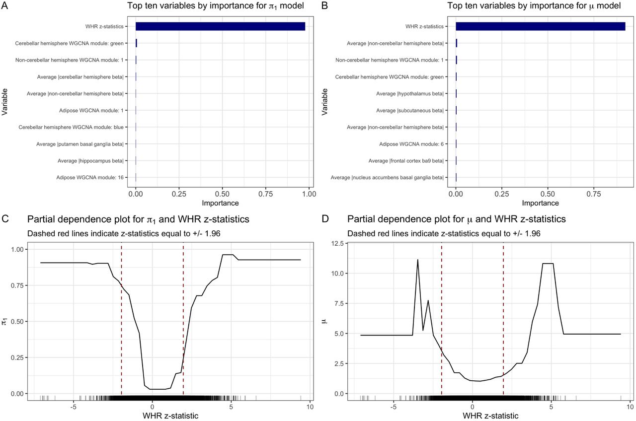
Variable importance plots for final BMI AdaPT (A) probability of being non-null and (B) effect size under alternative models. Partial dependence plot for both (C) probability of being non-null and (D) effect size under alternative with WHR z-statistics.
S7 CV tuning for SCZ, T2D, and BMI results
Rather than fixing the parameter settings for the XGBoost gradient boosted trees, we use the CV algorithm (detailed in Methods) at two steps of the search to tune the models (see the following section for justification of using two CV steps). For our search space, we evaluate a small range of values for the number of trees P and limit the maximum tree depth D to result in reasonably shallow trees (referred to as nrounds and max depth in the xgboost package (Chen et al. 2019)).
First, when exploring the improvement in discovery rate for the BrainVar eSNPs by incrementally including more information, we used the following XGBoost settings:
BD z-stats: Fixed D = 1, varied P ∈ {50, 100, 150},
BD z-stats + eQTL slopes: Combinations of P ∈ {100, 150}, D ∈ {1, 2},
BD z-stats + eQTL slopes + WGCNA: Combinations of P ∈ {100, 150}, D ∈ {2, 3},
WGCNA only: Combinations of P ∈ {100, 150}, D ∈ {1, 2, 3}.
We explored different settings for the different possible covariates to address the types of variables included. For instance, when using the BD z-statistics only, we considered single-split “stumps” to model the BD z-statistics relationships in purely an additive sense because it is a univariate example. Once we have all three types of covariates (BD z-statistics, eQTL slope summaries, and WGCNA results), we limit the maximum depth to be at least two to ensure possible interactions can be captured.
The selected number of trees P and maximum depth D for each of these sets of covariates is displayed in Table S1. For each set of the covariates, the most complex settings (largest number of trees and largest depth) are selected in both CV steps. This agreement in selection is not surprising given the choice of the low starting threshold s0 = 0.05, which differs from the results displayed in Table S3 of the next section using s0 = 0.45. We evaluated the same possible settings for the various all 2018 results displayed in Figures S5(C-D): the same choices for P and D displayed in Table S1 were selected in both CV steps.
For the SCZ results with the GTEx eSNPs using all covariates  , as well as the results for T2D and BMI with their full set of covariates, we evaluated four combinations: (1) P = 100, D = 2, (2) P = 150, D = 2, (3) P = 100, D = 3, and (4) P = 150, D = 3. For the BMI results using only WHR z-statistics, we fixed D = 1 and varied P ∈ {50, 100, 150}; for the results using WHR z-statistics with the eQTL slopes, we used combinations of P ∈ {100, 150}, D ∈ {1, 2}. The selected number of trees P and maximum depth D for each of these sets of AdaPT results at both CV steps is displayed in Table S2.
Selected boosting settings for number of trees P and maximum depth D with AdaPT CV algorithm by covariates for BrainVar eSNPs in each CV step.
Selected boosting settings for number of trees P and maximum depth D with AdaPT CV algorithm by GWAS results in each CV step.
S8 Selection of s0 and number of CV steps
To justify the selection of both the starting threshold s0 and number of CV steps for the AdaPT search, we generated simulations from the final AdaPT models returned from the SCZ 2014-only results. While these models are based on AdaPT results with a starting threshold of s0 = 0.05 and the use of two CV steps, they are only from the final model and are not explicitly parametrized by s0 and the number of CV steps. We know, however, that these final models are the result of using P = 150 trees with a maximum depth of D = 3, as indicated in Table S1 of the previous section.
Let  and
and  be the final models for the probability of non-null and effect size under the alternative that AdaPT returns for the BrainVar eSNPs using all covariates
  . We use these models as the “truth” for generating data, in which a single iteration of the simulation proceeds as follows:
For each BrainVar eSNP
Generate test status:
.Generate simulated effect sizes:
Transform to p-values pi.
Apply AdaPT to simulated study p-values with specified s0 and v CV steps with two candidate settings:
number of trees P = 100 and maximum depth D = 2,
number of trees P = 150 and maximum depth D = 3.
Compute observed power and FDP at range of target FDR α values.


We generate one-hundred simulations this way for each possible threshold s0 ∈ {0.05, 0.25, 0.45} and v ∈ {1, 2, 5} CV steps. Figure S16 displays the average difference in power between the different starting threshold values by the number of CV steps. Although the differences are small, we see that using s0 = 0.05 results in higher power, on average, than both 0.25 and the recommended 0.45 value. Using this low starting threshold of s0 = 0.05, we then directly compute the difference in power between the different number of CV steps displayed in Figure S17. Unsurprisingly, while again the differences are small, only one CV step results in the lowest power, on average. Since the computational cost of AdaPT with CV tuning is reduced by only using two CV steps instead of a higher number, such as five, and the simulations demonstrate on average no difference in power at both α values of 0.05 and 0.10, we use the starting threshold of s0 = 0.05 with two CV steps in our applications of AdaPT.
In the previous section, Table S1 displayed the selections in both CV steps with s0 = 0.05. For comparison, Table S3 displays the selections using s0 = 0.45. Instead of selecting the same settings in both steps, the higher initial threshold selects the least complex settings (smallest number of trees and minimum depth) in the first CV step before flipping to the most complex settings in the second step. Intuitively, the higher initial threshold means more information is masked from the models, so it is not surprising to see less complex settings chosen. This further reinforces the use of the lower initial threshold s0 = 0.05: it starts with more revealed information and selects model settings corresponding to improved CV performance for tests with lower p-values of interest.
Selected boosting settings for number of trees P and maximum depth D with AdaPT CV algorithm by covariates for BrainVar eSNPs with s0 = 0.45.

Difference in simulation power between different initial thresholds s0 for AdaPT search by number of CV steps. Points denote averages with plus/minus two standard error bars.

Difference in simulation power between the number of CV steps with s0 = 0.05. Points denote averages with plus/minus two standard error bars.
S9 Dependent p-value block simulation
To demonstrate the performance of AdaPT in the presence of dependent tests, we construct simulations with a block-correlation scheme to emulate LD structure for SNPs. We consider a setting with two independent covariates,

For each test i ∈ [n], we define a linear relationship for the log-odds of being non-null using these covariates,

Then, the resulting status of the test Hi is a Bernoulli random variable based on the probability π1,i(xi) where Hi = 1 indicates the test i is non-null while Hi = 0 indicates a true null,

Given this test status, a vector of true effect sizes µ = c(µi, …, µn) is also generated as a function of the covariates,

To simulate observed effect sizes, we construct an n × n covariance matrix Σ with B blocks of equal size  . Each block b ∈ [B] has constant correlation ρ between all tests within the block, while each block is independent of each other. This results in constructing individual block covariance matrices, Σb, with ones along the diagonal and ρ for the off-diagonal elements. Each of these individual matrices are placed along the diagonal of Σ, with the remaining off-diagonal elements set to zero so blocks are independent of each other. As an example, if each block contained only two tests they would be constructed in the following manner,

Using this block-wise construction of the covariance matrix, we then proceed to generate the vector of observed effect sizes z = (zi, …, zn) from a multivariate Gaussian distribution,

We compute the resulting two-side p-value pi = 2 · F(-|zi|) for each test’s observed effect size.
For each dataset generated using this process above, we compute both the observed FDP and power for the classical BH procedure and two different versions of AdaPT:
intercept-only,
gradient boosted trees with covariates: xi = (xi1, xi2).
We fix both n = 10,000 and B = 500 blocks, resulting in 500 blocks of twenty tests each. Rather than force all non-nulls together in the same blocks, we first calculate the minimum number of blocks required to hold all non-null tests,  . The non-null tests are then randomly assigned to
  blocks, ensuring that there will be blocks containing both null and non-null tests. The |{i: Hi = 0}| tests are randomly assigned to available spots within the BA blocks as well as the remaining 500 - BA strictly null blocks.
In our simulations, we fix β0 = -3 and require that both β1 = β2 and γ1 = γ2. We vary the following settings in our simulations:
block correlation ρ ∈ {0, 0.25, 0.5, 0.75, 1} where each block has the same value for ρ,
β1, β2 ∈ {1, 2, 3},
µfloor ∈ {0.5, 1, 1.5},
γ1, γ2 ∈ {0.5, .75, 1}.
We generate 100 simulations using the data generating process above, computing both the FDP and power for BH and the two different versions of AdaPT. For the covariate-informed version of AdaPT, we use gradient boosted trees via XGBoost with P = 100 trees and maximum depth D = 1. For both versions of AdaPT results, we start with the initial threshold of s0 = 0.45 and update the model ten times throughout the search (rather than the recommended twenty for computational speed).
Figures S18, S19, and S20 display points for the average observed FDP and power across the 100 simulations with plus/minus two standard errors bars for µfloor =0.5, 1, and 1.5 respectively, with target FDR level α = 0.05. The columns in each figure correspond to the different values considered for γ1 = γ2, while the rows correspond to β1 = β2. The x-axis for the figures displays the increasing block correlation ρ. Regardless of the simulation setting, we see that the AdaPT results when accounting for covariates (xi1, xi2) maintains valid FDR control at 0.05 similar to BH. This holds in the settings with greater effect sizes, as well as when the covariate information displays the best performance in terms of observed power (the bottom right panels of each figure). We can see that the intercept-only approach fails to achieve FDR control under block settings with perfect correlation, while the use of covariate information appears to inhibits such behavior. Our focus on positive correlation values is synonymous with the setting faced in genomics regarding LD structure. Further exploration of AdaPT’s performance in settings with arbitrary dependence structure presents an opportunity for future work, as well as accounting for covariate information that predict observed correlated noise.
S10 Simulations demonstrating effects of overfitting
It is possible that flexible methods like gradient boosted trees can be overfit, especially on small data sets. This could potentially lead to concerns about their incorporation in AdaPT. To assess the effects of overfitting the gradient boosted trees in AdaPT, we constructed simulated datasets using the finals models returned by AdaPT on the SCZ GWAS results,  and
and  , with the actual covariates
  for each of the
  eSNPs. We then simulated data using these models in the same manner previously explained for choosing s0 and the number of CV steps, and computed the observed power and FDP over a range of number of trees P ∈ {100, 300, 500, 700, 900}.
Figure S21(A) displays the distributions for fifty simulations of the observed FDP as the number of trees in the gradient boosted model increases. Regardless of the number of trees, we still maintain valid FDR control. However, Figure S21(B) shows as the number of trees increases, the method will overfit, resulting in a reduction in power. This reinforces that, although good model tuning can be important for power, the AdaPT method continues to maintain FDR control even as the model breaks down.
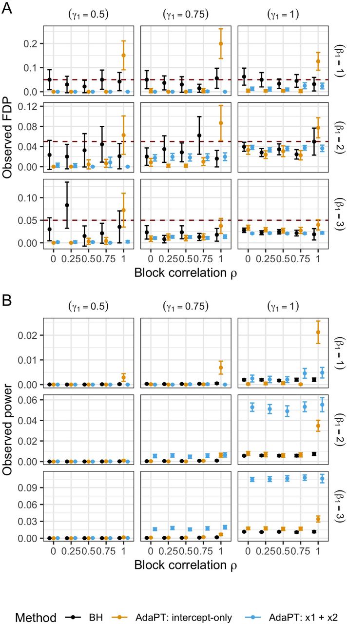
Comparison of average (A) FDP and (B) power with plus/minus two standard error bars for 100 simulations with µfloor = 0.5, and varying values for β1 (rows) and γ1 (columns) and block correlation ρ.

Comparison of average (A) FDP and (B) power with plus/minus two standard error bars for 100 simulations with µfloor = 1, and varying values for β1 (rows) and γ1 (columns) and block correlation ρ.

Comparison of average (A) FDP and (B) power with plus/minus two standard error bars for 100 simulations with µfloor = 1.5, and varying values for β1 (rows) and γ1 (columns) and block correlation ρ.
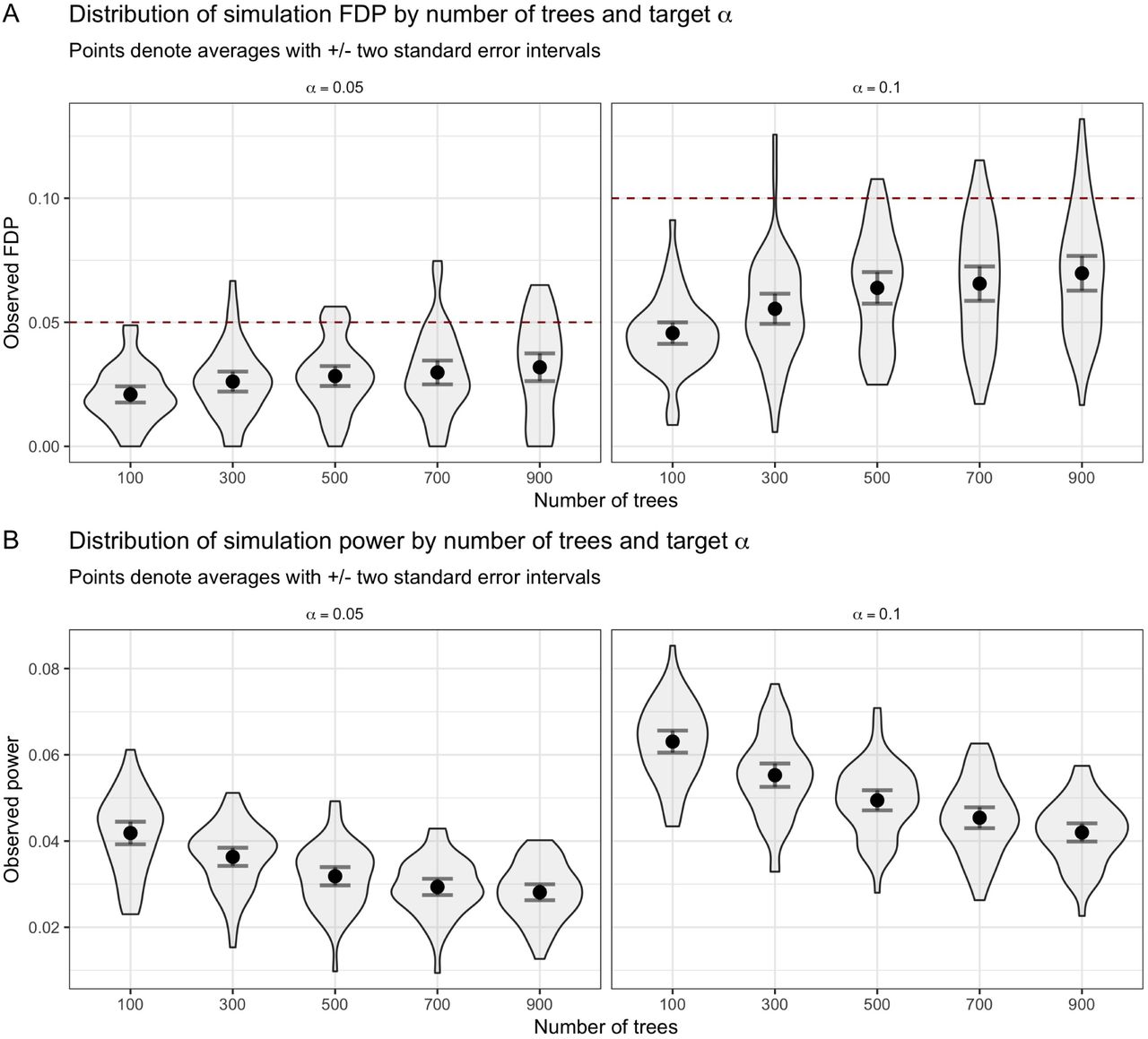
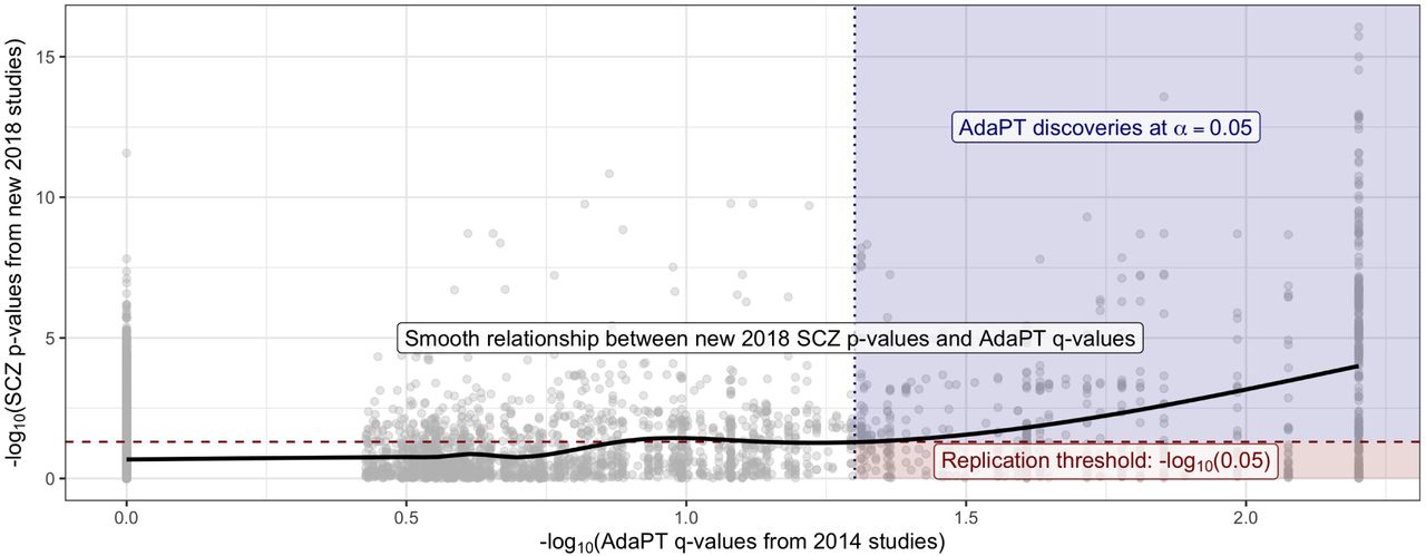
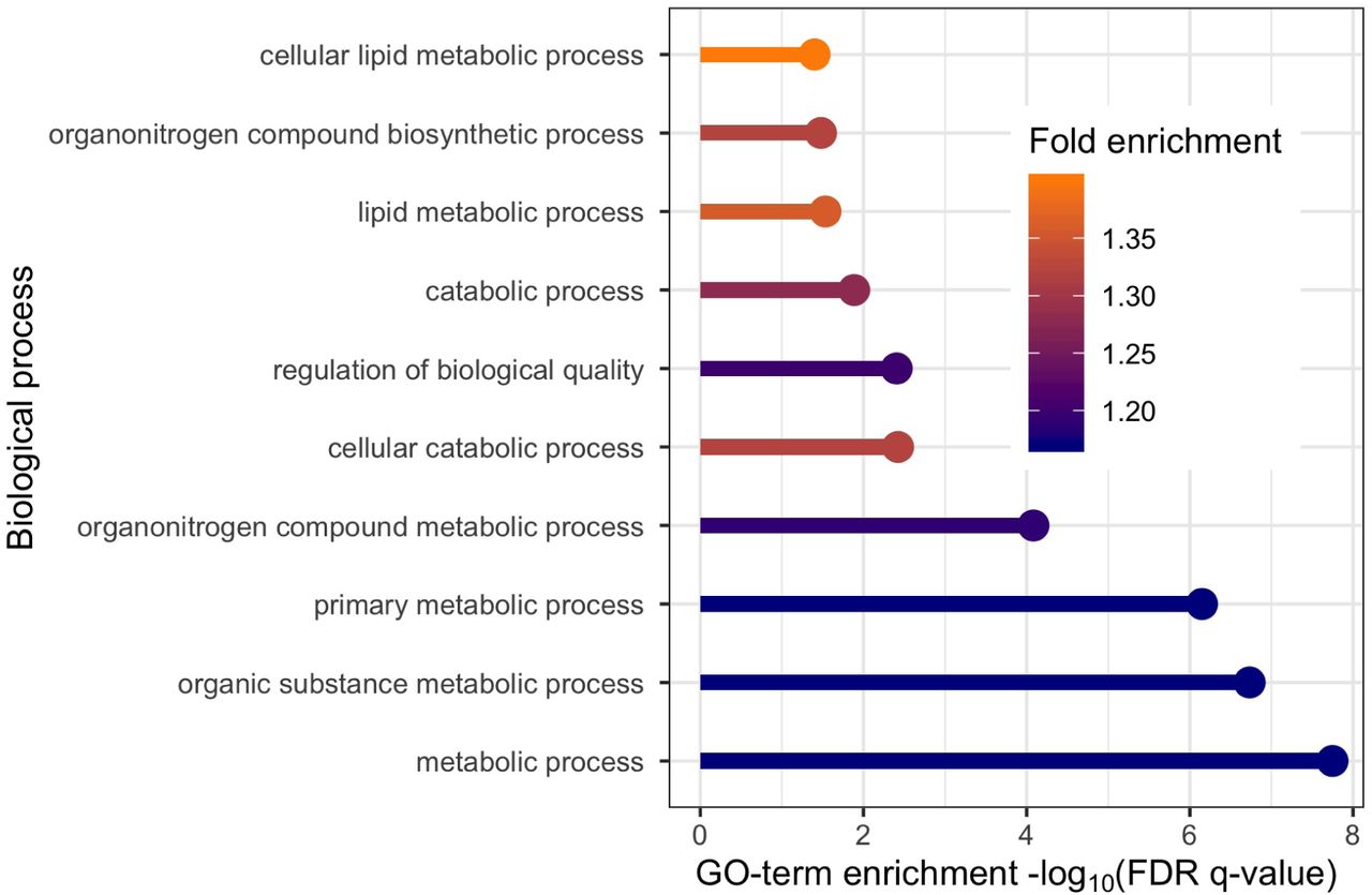
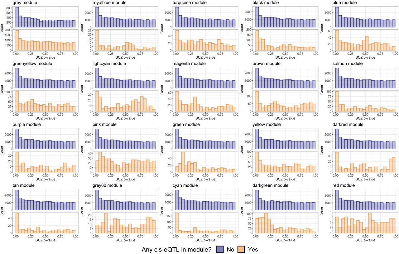
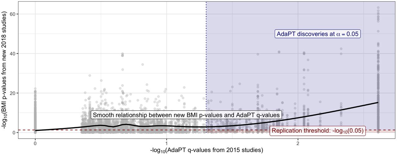
Distributions of observed (A) FDP and (B) power for simulations as the number of AdaPT gradient boosted trees increases by target FDR level α. Points denote averages with plus/minus two standard error intervals.
Footnotes
References


