

Abstract
Antimicrobial resistance is an increasing threat to global health. Evidence for this trend is generated in microbiological laboratories through testing microorganisms for resistance against antimicrobial agents. International standards and guidelines are in place for this process as well as for reporting data on (inter-)national levels. However, there is a gap in the availability of standardized and reproducible tools for working with laboratory data to produce the required reports. Of data coming from laboratory information systems, it is known that extensive efforts in data cleaning and validation are required. Furthermore, the global nature of antimicrobial resistance demands to incorporate international reference data in the analysis process.
In this paper, we introduce the AMR package for R that aims at closing this gap by providing tools to simplify antimicrobial resistance data cleaning and analysis, while incorporating international guidelines and scientifically reliable reference data. The AMR package enables standardized and reproducible antimicrobial resistance analyses, including the application of evidence-based rules, determination of first isolates, translation of various codes for microorganisms and antimicrobial agents, determination of (multi-drug) resistant microorganisms, and calculation of antimicrobial resistance, prevalence and future trends. The AMR package works independently of any laboratory information system and provides several functions to integrate into international workflows (e.g. WHONET software by the World Health Organization).
1. Introduction
Antimicrobial resistance is a global health problem and of great concern for human medicine, veterinary medicine, and the environment alike. It is associated with significant economic burdens to both patients and health care systems. Current estimates show the immense dimensions we are already facing, such as claiming at least 50,000 lives due to antimicrobial resistance each year across Europe and the US alone (O’Neill 2014). Although estimates for the burden through antimicrobial resistance and their predictions are disputed (de Kraker et al. 2016) the rising trend is undeniable, thus calling for worldwide efforts on tackling this problem.
Surveillance programs and reliable data are key for controlling and streamlining these efforts. Surveillance data of antimicrobial resistance at higher levels (national or international) usually comprise aggregated numbers. The basis of this information is generated and stored at microbiological laboratories where isolated microorganisms are tested for their susceptibility to a whole range of antimicrobial agents. The efficacy of these agents is interpreted as “susceptible” (S), “intermediate” (I) or “resistant” (R) by guidelines. Today, the two major guideline institutes to define the international standards are the European Committee on Antimicrobial Susceptibility Testing (EUCAST) (Leclercq et al. 2013) and the Clinical and Laboratory Standards Institute (CLSI) (Clinical and Laboratory Standards Institute 2014). (Recently, EUCAST changed the interpretation of S, I and R, but this paper still follows the traditional, wider known definitions above). The guidelines from these two institutes are adopted by 94% of all countries reporting antimicrobial resistance to the WHO (World Health Organization 2018a).
Although these standardized guidelines are in place on the laboratory level for the data generation process, stored data in laboratory information systems are often not yet suitable for data analysis. Laboratory information systems are often designed to fit billing purposes rather than epidemiological data analysis. Furthermore, (inter-)national surveillance is hindered by inadequate standardization of epidemiological definitions, different types of samples and data collection, settings included, microbiological testing methods (including susceptibility testing), and data sharing policies (Tacconelli et al. 2018). The necessity of accurate data analysis in the field of antimicrobial resistance has just recently been further underlined (Limmathurotsakul et al. 2019).
Here, we describe the AMR package for R, which has been developed to simplify antimicrobial resistance data cleaning and analysis using international standardized recommendations (Leclercq et al. 2013; Clinical and Laboratory Standards Institute 2014) while incorporating scientifically reliable reference data about valid laboratory outcome, antimicrobial agents, and the complete biological taxonomy of microorganisms. This package is available on the Comprehensive R Archive Network (CRAN) since February 22nd, 2018. To the best of our knowledge, no other R packages with this purpose are available on CRAN or Bioconductor.
Antimicrobial resistance analyses require a thorough understanding of microbiological tests and their results, the biological taxonomy of microorganisms, the clinical and epidemiological relevance of the results, their pharmaceutical implications, and (inter-)national standards and guidelines for working with and reporting antimicrobial resistance. The AMR package provides solutions and support for all these aspects while being independent of underlying laboratory information systems, thereby democratizing the analysis process. Developed in R, the AMR package enables reproducible workflows as described in other fields, such as environmental science (Lowndes et al. 2017). The AMR package could be a new technical instrument to aid in curbing the global threat of antimicrobial resistance.
The following sections describe the functionality of the AMR package according to its core functionalities for transforming, enhancing, and analyzing antimicrobial resistance data using scientifically reliable reference data.
2. Antimicrobial resistance data
Microbiological tests can be performed on different specimens, such as blood or urine samples or nasal swabs. After arrival at the microbiological laboratory, the specimens are traditionally cultured on specific media, such as blood agar. If a microorganism can be isolated from these media it is tested against several antimicrobial agents. Based on the minimal inhibitory concentration (MIC) of the respective drug and interpretation guidelines, e.g. guidelines by EUCAST (Leclercq et al. 2013) or CLSI (Clinical and Laboratory Standards Institute 2014), test results are reported as “susceptible” (S), “intermediate” (I) or “resistant” (R). A typical data structure is illustrated in Table 1 (Leclercq et al. 2013).
Example of an antimicrobial resistance report.
For the first two rows, the information should be read as: Escherichia coli (mo code = esccol) was isolated from blood of patient 000001 and was found to be resistant to penicillin, intermediate to amoxicillin/clavulanic acid, and susceptible to ciprofloxacin. However, often (especially when merging sources) data is reported in ambiguous formats as exemplified in Table 2.
Antimicrobial resistance report example – ambiguous formats.
The AMR package aims at providing a standardized and automated way of cleaning, transforming, and enhancing these typical data structures (Table 1 and 2), independent of the underlying data source. Processed data would be similar to Table 3 that highlights several package functionalities in the sections below.
Enhanced antimicrobial resistance report example.
3. Antimicrobial resistance data transformation
The AMR package follows the rationale of tidyverse packages as authored by Wickham (2017). Most functions take a ‘data.frame’ or ‘tibble’ as input, support piping (%>%) operations, can work with quasi-quotations, and can be integrated into dplyr workflows, such as mutate() to create new variables.
3.1. Working with taxonomically valid microorganism names
Coercing is a computational process of forcing output based on an input. For microorganism names, coercing user input to taxonomically valid microorganism names is crucial to ensure correct interpretation and to enable grouping based on taxonomic properties. To this end, the AMR package includes all microbial entries from The Catalogue of Life (http://www.catalogueoflife.org), the most comprehensive and authoritative global index of species currently available (Roskov Y., Ower G., Orrell T., Nicolson D., Bailly N., Kirk P.M., Bourgoin T., DeWalt R.E., Decock W., Nieukerken E. van, Zarucchi J., Penev L. 2019). It holds essential information on the names, relationships, and distributions of in total more than 1.9 million species. The partial integration of it into the AMR package is described in Section 8.
The as.mo() function makes use of this underlying data to transform a vector of characters to a new class ‘mo’ of taxonomically valid microorganism name. The resulting values are microbial IDs, which are human-readable for the trained eye and contain information about the taxonomic kingdom, genus, species, and subspecies (Figure 1).

The structure of a typical microbial ID as used in the AMR package. An ID consists of two to four elements, separated by an underscore. The first element is the abbreviation of the taxonomic kingdom. The remaining elements consist of abbreviations of the lowest taxonomic levels of every microorganism: genus, species (if available) and subspecies (if available). Abbreviations used for the microbial IDs of microorganism names were created using the base R function abbreviate().
The as.mo() function uses several coercion rules for fast and logical results. It assesses the input matching criteria in the following order:
Human pathogenic prevalence: the function starts with more prevalent microorganisms, followed by less prevalent ones;
Taxonomic kingdom: the function starts with determining Bacteria, then Fungi, then Protozoa, then others;
Breakdown of input values to identify possible matches.
This will lead to the effect that e.g. “E. coli” (a highly prevalent microorganism found in humans) will return the microbial ID of Escherichia coli and not Entamoeba coli (a less prevalent microorganism in humans), although the latter would alphabetically come first. In addition, the as.mo() function can differentiate four levels of uncertainty to guess valid results:
Uncertainty level 0: no additional rules are applied;
Uncertainty level 1: allow previously accepted (but now invalid) taxonomic names and minor spelling errors;
Uncertainty level 2 (default): allow all of level 1, strip values between brackets, inverse the words of the input, strip off text elements from the end keeping at least two elements;
Uncertainty level 3: allow all of level 1 and 2, strip off text elements from the end, allow any part of a taxonomic name.
These rules consider the prevalence of microorganisms in humans. The grouping into three prevalence groups is based on experience from several microbiological laboratories in the Netherlands in conjunction with international reports on pathogen prevalence (de Greeff et al. 2019; European Centre for Disease Prevention and Control 2010; World Health Organization 2018a). Group 1 (most prevalent microorganisms) consists of all microorganisms where the taxonomic class is Gammaproteobacteria or where the taxonomic genus is Enterococcus, Staphylococcus or Streptococcus. This group consequently contains all common Gram-negative bacteria, such as Pseudomonas and Legionella and all species within the order Enterobacteriales. Group 2 consists of all microorganisms where the taxonomic phylum is Proteobacteria, Firmicutes, Actinobacteria or Sarcomastigophora, or where the taxonomic genus is Absidia, Acremonium, Actinotignum, Alternaria, Anaerosalibacter, Apophysomyces, Arachnia, Aspergil lus, Aureobacterium, Aureobasidium, Bacteroides, Basidiobolus, Beauveria, Blastocystis, Branhamella, Calymmatobacterium, Candida, Capnocytophaga, Catabacter, Chaetomium, Chryseobacterium, Chryseomonas, Chrysonilia, Cladophialophora, Cladosporium, Conidiobolus, Cryptococcus, Curvularia, Exophiala, Exserohilum, Flavobacterium, Fonsecaea, Fusarium, Fusobacterium, Hendersonula, Hypomyces, Koserella, Lelliottia, Leptosphaeria, Leptotrichia, Malassezia, Malbranchea, Mortierel la, Mucor, Mycocentrospora, Mycoplasma, Nectria, Ochroconis, Oidiodendron, Phoma, Piedraia, Pithomyces, Pityrosporum, Prevotella, Pseudallescheria, Rhizomucor, Rhizopus, Rhodotorula, Scolecobasidium, Scopulariopsis, Scytalidium, Sporobolomyces, Stachybotrys, Stomatococcus, Treponema, Trichoderma, Trichophyton, Trichosporon, Tritirachium or Ureaplasma. Group 3 consists of all other microorganisms.
To support organization specific codes, users can specify a custom reference ‘data.frame’ for looking up codes, that can be set with as.mo(…, reference_df = …). This process can be automated by users with the set_mo_source() function.
Properties of microorganisms
The package contains functions to return a specific (taxonomic) property of a microorganism from the microorganisms data set (see Section 8). Using functions that start with mo_* can be used to retrieve the most recently defined taxonomic properties of any microorganism quickly and conveniently. These functions rely on as.mo() internally: mo_name(), mo_fullname(), mo_shortname(), mo_subspecies(), mo_species(), mo_genus(), mo_family(), mo_order(), mo_class(), mo_phylum(), mo_kingdom(), mo_type(), mo_gramstain(), mo_ref(), mo_authors(), mo_year(), mo_rank(), mo_taxonomy(), mo_synonyms(), mo_info() and mo_url(). Determination of the Gram stain, with mo_gramstain(), is based on the taxonomic subkingdom and phylum. According to Cavalier-Smith (2002), who defined the subkingdoms Negibacteria and Posibacteria, only the following phyla are Posibacteria: Actinobacteria, Chloroflexi, Firmicutes and Tenericutes. Bacteria from these phyla are considered Gram-positive – all other bacteria are considered Gram-negative. Gram stains are only relevant for species within the kingdom of Bacteria. For species outside this kingdom, mo_gramstain() will return NA.
3.2. Working with antimicrobial names or codes
The AMR package includes the antibiotics data set, which comprises common laboratory information system codes, official names, ATC (Anatomical Therapeutic Chemical) codes, defined daily doses (DDD) and more than 5,000 trade names of 452 antimicrobial agents (see Section 8). The ATC code system and the reference list for DDDs have been developed and made available by the World Health Organization Collaborating Centre for Drug Statistics Methodology (WHOCC) to standardize pharmaceutical classifications (WHO Collaborating Centre for Drug Statistics Methodology 2018). All agents in the antibiotics data set have a unique antimicrobial ID, which is based on abbreviations used by the European Antimicrobial Resistance Surveillance Network (EARS-Net), the largest publicly funded system for antimicrobial resistance surveillance in Europe (European Centre for Disease Prevention and Control 2018).
Properties of antimicrobial agents
It is a common task in microbiological data analyses (and other clinical or epidemiological fields) to work with different antimicrobial agents. The AMR package provides several functions to translate inputs such as ATC codes, abbreviations, or names in any direction. Using as.ab(), any input will be transformed to an antimicrobial ID of class ‘ab’. Helper functions are available to get specific properties of antimicrobial IDs, such as ab_name() getting the official name, ab_atc() the ATC code, or ab_cid() the CID (Compound ID) used by Pub-Chem (Kim et al. 2019). Trade names can be also used as input. For example, the input values “Amoxil”, “dispermox”, “amox” and “J01CA04” all return the ID of amoxicillin (AMX): R> as.ab(“Amoxicillin”) Class ‘ab’ [1] AMX R> as.ab(c(“Amoxil”, “dispermox”, “amox”, “J01CA04”)) Class ‘ab’ [1] AMX AMX AMX AMX R> ab_name(“Amoxil”) [1] “Amoxicillin” R> ab_atc(“amox”) [1] “J01CA04” R> ab_name(“J01CA04”) [1] “Amoxicillin”
Filtering data based on classes of antimicrobial agents
The application of the ATC classification system also enables grouping of antimicrobial agents for data analyses. Data sets with microbial isolates can be filtered on isolates with specific results for tested antimicrobial agents in a specific antimicrobial class. For example, using filter_cephalosporins(result = “R”) returns data of all isolates with tested resistance to any of the available antimicrobial agents in in the group of cephalosporins.
3.3. Other new S3 classes
S3 classes are object oriented (OO) systems available in R. The classes ‘mo’ and ‘ab’ that are discussed above are S3 classes, which means that they allow different types of output based on the user input. Three other new S3 classes that come with this package are ‘mic’, ‘disk’, and ‘rsi’. The ‘mic’ class can be used to clean MIC (minimal inhibitory concentration) values. MIC values are susceptibility test results measured by microbiological laboratory equipment to determine at which minimum antimicrobial drug concentration 99.9% of a microorganism is inhibited in growth. These concentrations are often capped at a minimum and maximum, such as <= 0.02 mg/ml and >= 32 mg/ml, respectively. The ‘mic’ class, an ordered ‘factor’, keeps these operators while still ordering all possible outcomes correctly, so that e.g. “<= 0.02” will be considered lower than “0.04”.
Another susceptibility testing method is the use of drug diffusion disks, which are small tablets containing a specified concentration of antimicrobial agents. These disks are are applied onto a solid growth medium, or a specific agar plate. After 24 hours of incubation, the diameter of the growth inhibition around a disk can be measured in millimeters with a ruler. The ‘disk’ class can be used to clean these kinds of measurements, since they should always be valid numeric values between 8 and 50.
The higher the MIC or the smaller the growth inhibition diameter, the more active substance of an antimicrobial drug is needed to inhibit cell growth (i.e. the higher the antimicrobial resistance of the tested isolate against the tested antimicrobial agent). At low MICs and wide diameters, guidelines interpret the microorganism as susceptible (S) to the tested antimicrobial agent. At high MICs and small diameters, guidelines interpret the microorganism as resistant (R) to the tested antimicrobial agent. In between, the microorganism is classified as intermediate (I). For these three interpretations the ‘rsi’ class has been developed. When using as.rsi() on MIC values (of class ‘mic’) or disk diffusion diameters (of class ‘disk’), the values will be interpreted according to the guidelines from the CLSI or EUCAST (all guidelines between 2011 and 2019 are included in the AMR package) (Clinical and Laboratory Standards Institute 2019; The European Committee on Antimicrobial Susceptibility Testing 2019). Guidelines can be changed by setting the guidelines argument. When using the as.rsi() function on existing antimicrobial interpretations, it tries to coerce the input to the values “S”, “I”, or “R”. These values can in turn be used to calculate the proportion of antimicrobial resistance.
3.4. Interpretative rules by EUCAST
Next to supplying guidelines to interpret raw MIC values, the EUCAST has developed a set of expert rules to assist clinical microbiologists in the interpretation and reporting of antimicrobial susceptibility tests (Leclercq et al. 2013). The rules comprise assistance on intrinsic resistance, exceptional phenotype, and interpretive rules. The AMR package covers intrinsic resistant and interpretive rules for data transformation and standardization purposes. The first prevents false susceptibility reporting by providing a list of organisms with known intrinsic resistance to specific antimicrobial agents (e.g. cephalosporin resistance of all enterococci). Interpretative rules apply inference from established resistance mechanisms (Winstanley and Courvalin 2011; Courvalin 1992, 1996; Livermore et al. 2001). Both groups of rules are based on classic IF THEN statements (e.g. IF Enterococcus spp. resistant to ampicillin THEN report as resistant to carbapenems). Some rules provide assistance for further actions when a certain resistance has been found, i.e. performing additional testing of the isolated microorganism. The AMR package function eucast_rules() can apply all EUCAST rules that do not rely on additional clinical information, such as patients having a urinary tract infection. Applied changes can be reviewed by setting the argument eucast_rules(…, verbose = TRUE). Table 2 and 3 highlight the transformation for the reporting of AMX = S in patient_id = 000003 to the correct report according to EUCAST rules of AMX = R.
3.5. Working with defined daily doses (DDD)
DDDs are essential when standardizing antimicrobial consumption analysis for inter-institutional or international comparison. The official DDDs are published by the WHOCC and subject to regular updates (WHO Collaborating Center for Drug Statistics Methodology 2019). Other metrics exist such as the recommended daily dose (RDD) or the prescribed daily dose (PDD). However, DDDs are the only metric that is independent of a patient’s disease and therapeutic choices and thus suitable for the AMR package.
Functions from the atc_online_*() family take any text as input that can be coerced with as.ab() (i.e. to class ‘ab’). Next, the functions access the WHOCC online registry (WHO Collaborating Center for Drug Statistics Methodology 2019) (internet connection required) and download the property defined in the arguments (e.g. administration = “O” or administration = “P” for oral or parenteral administration and property = “ddd” or property = “groups” to get DDD or the group of the selected antimicrobial defined by its ATC code). R> atc_online_ddd(“amoxicillin”, administration = “O”) [1] 1.5 R> atc_online_groups(“amoxicillin”) [1] “ANTIINFECTIVES FOR SYSTEMIC USE” [2] “ANTIBACTERIALS FOR SYSTEMIC USE” [3] “BETA-LACTAM ANTIBACTERIALS, PENICILLINS” [4] “Penicillins with extended spectrum”
4. Enhancing antimicrobial resistance data
4.1. Determining first isolates
Determining antimicrobial resistance or susceptibility can be done for a single drug (monotherapy) or multiple drugs (combination therapy). The calculation of antimicrobial resistance statistics is dependent on two prerequisites: the data should only comprise the first isolates and a minimum required number of 30 isolates should be met for every stratum in further analysis (Clinical and Laboratory Standards Institute 2014).
An isolate is a microorganism strain cultivated on specified growth media in a laboratory, so its phenotype can be determined. First isolates are isolates of any species found first in a patient per episode, regardless of the body site or the type of specimen (such as blood or urine) (Clinical and Laboratory Standards Institute 2014). The selection on first isolates (using function first_isolate()) is important to prevent selection bias, as it would lead to overestimated or underestimated resistance of an antimicrobial agent. For example, if a patient is admitted with a multi-drug resistant microorganism and that microorganism is found in five different blood cultures the following week, it would overestimate resistance if all isolates were to be counted. The episode in days can be set with the argument episode_days, which defaults to 365 as suggested by the Clinical and Laboratory Standards Institute (2014) guideline.
4.2. Determining multi-drug resistant organisms (MDRO)
Definitions of multi-drug resistant organisms (MDRO) are regulated by national and international expert groups and differ between nations. The AMR package provides the functionality to quickly identify MDROs in a data set using the mdro() function. Guidelines can be set with the argument guideline. At default, it applies the guideline as proposed by Magiorakos et al. (2012). Their work describes the definitions for bacteria being ‘MDR’ (multi-drug-resistant), ‘XDR’ (extensively drug-resistant) or ‘PDR’ (pandrug-resistant). These definitions are widely adopted (Abat et al. 2018) and known in the field of medical microbiology.
Other guidelines currently supported are the international EUCAST guideline (guideline = “EUCAST”, European Committee on Antimicrobial Susceptibility Testing (EUCAST) (2016)), the international WHO guideline on the management of drug-resistant tuberculosis (guideline = “TB”, World Health Organization (2014)), and the national guidelines of The Netherlands (guideline = “NL”, Werkgroep Infectiepreventie (WIP) (2011)) and Germany (guideline = “DE”, Müller et al. (2015)).
Some guidelines require a minimum availability of tested antimicrobial agents per isolate. This is needed to prevent false-negatives, since no reliable determination can be performed on only a few test results. This required minimum defaults to 50%, but can be set by the user with the pct_minimum_classes. Isolates that do not meet this requirement will be skipped for determination and will return NA (not applicable), with an informative warning printed to the console.
The rules are applied per row of the data. The mdro() function automatically identifies the variables containing the microorganism codes and antimicrobial agents based on the guess_ab_col() function. Following a guideline set by the user, it analyses the specific antimicrobial resistance of a microorganism and flags that microorganism accordingly. The outcome of this function is always a ‘factor’ and is demonstrated in Table 4.
Example of a multi-drug resistant organism (MDRO) in a data set identified by applying Dutch guidelines.
According to the Dutch guidelines Werkgroep Infectiepreventie (WIP) (2011), the first row is an MDRO since it is resistant to the antimicrobial groups of aminoglycosides (gentamcin, tobramycin) and fluoroquinolones (ciprofloxacin, moxifloxacin). The returned value is an ordered ‘factor’ with the levels ‘Negative’ < ‘Positive, unconfirmed’ < ‘Positive’. For some guideline rules that require additional testing (e.g. molecular confirmation), the level ‘Positive, unconfirmed’ is returned.
Multi-drug resistant tuberculosis
Tuberculosis is a major threat to global health caused by Mycobacterium tuberculosis (MTB) and is one of the top ten causes of death worldwide (World Health Organization 2018b). Exceptional antimicrobial resistance in MTB is therefore of special interest. To this end, the international WHO guideline for the classification of drug resistance in MTB (World Health Organization 2014) is included in the AMR package. The mdr_tb() function is a convenient wrapper around mdro(…, guideline = “TB”), which returns an other ordered ‘factor’ than other mdro() functions. The output will contain the ‘factor’ levels ‘Negative’ < ‘Mono-resistant’ < ‘Poly-resistant’ < ‘Multi-drug-resistant’ < ‘Extensive drugresistant’ following the WHO guideline.
5. Analyzing antimicrobial resistance data
5.1. Calculation of antimicrobial resistance
The AMR package contains several functions for fast and simple resistance calculations of bacterial or fungal isolates. A minimum number of available isolates is needed for the reliability of the outcome. The CLSI guideline suggests a minimum of 30 available first isolates irrespective of the type of statistical analysis (Clinical and Laboratory Standards Institute 2014). Therefore, this number is used as the default setting for any function in the package that calculates antimicrobial resistance or susceptibility.
Counts
The AMR package relies on the concept of tidy data (Wickham 2014), although not strictly following its rules (one row per test rather than one row per observation). Function names to calculate the number of available isolates follow these general resistance interpretation standards with count_S(), count_I(), and count_R() respectively. Combinations of antimicrobial resistance interpretations can be counted with count_SI() and count_IR(). All these functions take a vector of interpretations of the class ‘rsi’ (as discussed above) or are internally transformed with as.rsi(). The returned value is the sum of the respective interpretation in the selected test column. All count_*() functions support quasi-quotation with pipes, grouped variables, and can be used with dplyr::summarise() (Wickham et al. 2019).
Proportions
Calculation of antimicrobial resistance is carried out by counting the number of first resistant isolates (interpretation of “R”) and dividing it by the number of all first isolates, see Formula 1. This is implemented in the portion_R() function. To calculate antimicrobial susceptibility, the number of susceptible first isolates (interpretation of “S”) has to be counted and divided by the number of all first isolates with portion_S().
 where x is an antimicrobial agent, z is an antimicrobial interpretation (“S”, “I”, or “R”) and R is the antimicrobial resistance.
The functions portion_S(), portion_I(), portion_R(), portion_SI(), and portion_IR() follow the same logic as the count_*() functions and all return a vector of class ‘double’ with values between 0 and 1. The argument minimum defines the minimal allowed number of available (tested) isolates (default: minimum = 30). Any total isolate number lower than minimum will return NA with a warning.
For the proportion of empiric susceptibility for more than one antimicrobial agent, the total number of first isolates where at least one agent was tested as “S” or “I” must be divided by the number of first isolates tested where all agents were tested for any interpretation (see Formula 2 and Table 5).
 where x and y are antimicrobial agents, z is an antimicrobial interpretation: “S”, “I”, or “R” and R is the antimicrobial resistance.
Example calculation for determining empiric susceptibility (%SI) for more than one antimicrobial agent.
Based on Formula 1, the overall resistance and susceptibility of an antimicrobial agent like gentamicin (GEN) can be calculated using the following syntax (an example data set is included in the AMR package, containing test results of 2000 isolates: example_isolates): R> library(“dplyr”) R> example_isolates %>% + summarise(r_gen = portion_R(GEN), + si_gen = portion_SI(GEN), + count_gen = n_rsi(GEN)) r_gen si_gen count_gen 1 0.2458221 0.7541779 1855
This output reads: the resistance against gentamicin of all isolates in the example_isolates data set is RGEN = 24.6%, based on 1855 out of 2000 available isolates. The susceptibility is 1 – RGEN = 75.4%.
To calculate the effect of combination therapy, i.e. treating patients with multiple agents at the same time, the portion_SI() can handle multiple variables as arguments. For example, to calculate the empiric susceptibility of a combination therapy comprising gentamicin (GEN) and amoxicillin (AMX): R> example_isolates %>% + summarise(si_gen_amx = portion_SI(GEN, AMX), + count_gen_amx = n_rsi(GEN, AMX)) si_gen_amx count_gen_amx 1 0.9328603 1919
This leads to the conclusion that combining gentamicin with amoxicillin would cover 1 – RGEN, AMX = 93.3% based on 1919 out of 2000 available isolates, which is 17.9% more than when treating with gentamicin alone (1 – RGEN = 75.4%). With these functions, exact calculations can be done to evaluate the empiric success of inhibiting growth of microorganisms, by treating them with specified antimicrobial agents.
5.2. Prediction of antimicrobial resistance
The AMR package can handle several different regression models that can be used to predict antimicrobial resistance. The resistance_predict() function uses dates (argument col_date) and a selected antimicrobial agent (argument col_ab) to estimate resistance rates of a specified number of upcoming years (default: year_max = 10). The user needs to specify the statistical model by setting the model argument. Valid options are generalized linear models with a binomial distribution or Poisson distribution, or a linear regression model. Furthermore, it is required to decide on the choice of interpreting isolates with intermediate resistance as susceptible isolates (default: I_as_S = TRUE). The minimum number of isolates per year defaults to 30 and can be set with the minimum argument.
The resistance_predict() function returns a ‘data.frame’ with an extra S3 class ‘resistance_predict’ and contains the following columns: year, value, se_min (the lower bound of the standard error with a minimum of 0), se_max (the upper bound of the standard error with a maximum of1), observations (the total number of observations in the respective year, i.e. “S” + “I” + “R”), observed (the original observed resistant percentages), and estimated (the estimated resistant percentages calculated by the model). Furthermore, the model itself is available as an attribute: attributes(x)$model.
5.3. Plotting of antimicrobial resistance
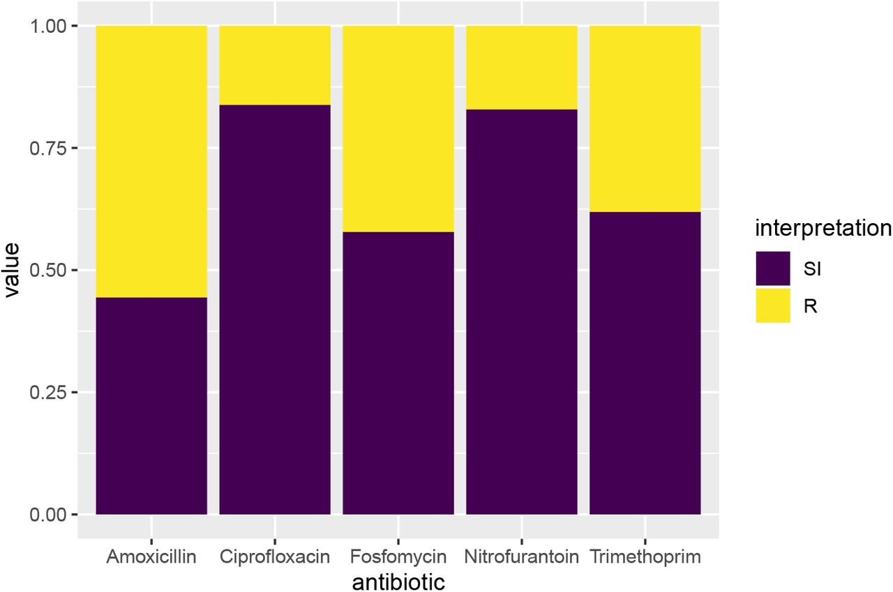
The AMR package contains simple plotting functionalities to visualize antimicrobial resistance data. The geom_rsi() function for plotting data containing antimicrobial test results is extending the ggplot2 package (Wickham 2016) with a new so-called ‘geom’, geom_rsi(). The output is fully editable and follows the common ggplot2 code. Arguments include position, fill, and facets (relying on ggplot2::facet_wrap()). Moreover, the argument translate_ab uses ab_name() to translate abbreviations of antimicrobial agents into official names. Figure 2 demonstrates an example plotting function with a selection of antimicrobial agents commonly used to treat urinary tract infections. R> library(ggplot2) R> example_isolates %>% + select(AMX, NIT, FOS, TMP, CIP) %>% + ggplot() + + geom_rsi()

Selection of five variables from the example_isolates data set: AMX (amoxicillin), NIT (nitrofurantoin), FOX (fosfomycin), TMP (trimethoprim) and CIP (ciprofloxacin). These variables are passed onto ggplot() and the new ‘geom’ geom_rsi(), that automatically calculates antimicrobial resistance, translates the abbreviations of antimicrobial agents and plots the data.
In addition, the ggplot_rsi() function provides a wrapper around the geom_rsi() function, taking any kind of ‘data.frame’ as first input, so the function can be used after a pipe (%>%).
Prediction analyses can also be visualized with the AMR package. It extends the base R function plot(), but also contains a ggplot2 wrapper with the function ggplot_rsi_predict() as shown in Figure 3. R> example_isolates %>% + resistance_predict(col_ab = “TZP”, + model = “binomial”) %>% + ggplot_rsi_predict()

Prediction of antimicrobial resistance to the TZP (piperacillin/tazobactam) variable from the example_isolates data set. A regression model with a binomial cumulative distribution function was chosen, assuming a period of very low resistance that cumulatively increases over time. The ggplot_rsi_predict() function calculates the antimicrobial resistance per year and plots the observations, followed by a prediction of the upcoming years. The grey ribbon denotes the standard error of the mean, calculated as  .
.
6. Reproducible example
A completely worked out example with fully annotated R code is available as supplementary material, with file name complete_reproducible_example.R.
7. Summary
This paper demonstrates the AMR package and its foremost use for working with antimicrobial resistance data. It can be used to clean, enhance, and analyse such data according to international recommendations and guidelines while incorporating scientifically reliable reference data on microbiological laboratory test results, antimicrobial agents, and the biological taxonomy of microorganisms. Consequently, it especially allows for reproducible analyses, regardless of the many possible ways in which raw and uncleaned data are stored in laboratory information systems.
While the burden of antimicrobial resistance is continuing to increase worldwide, reliable data and data analyses are needed to better understand current and future developments. Open source approaches, such as the AMR package for R, have the potential to help democratizing the required tools in the field for researchers, clinicians, and policy makers alike.
8. Included data sets
antibiotics
A ‘data.frame’ containing 452 antimicrobial agents with 13 columns. All entries in this data set have three different identifiers: a human readable EARS-Net code (as used by ECDC (European Centre for Disease Prevention and Control 2010) and WHONET (WHO Collaborating Centre for Surveillance of Antimicrobial Resistance 2019) and primarily used by this package), an ATC code (as used by the WHO (WHO Collaborating Centre for Drug Statistics Methodology 2018)), and a CID code (Compound ID, as used by PubChem (Kim et al. 2019)). The data set contains more than 5,000 official brand names from many different countries, as found in PubChem. Other properties in this data set are derived from one or more of these codes, such as official names of pharmacological and chemical subgroups, and defined daily doses (DDD).
microorganisms
A ‘data.frame’ containing 69,447 (sub)species with 16 columns comprising their complete microbial taxonomy according to the Catalogue of Life (Roskov Y., Ower G., Orrell T., Nicolson D., Bailly N., Kirk P.M., Bourgoin T., DeWalt R.E., Decock W., Nieukerken E. van, Zarucchi J., Penev L. 2019). Included microorganisms and their complete taxonomic tree of all included (sub)species from kingdom to subspecies with year of scientific publication and responsible author(s):
– All 57,776 (sub)species from the kingdoms of Archaea, Bacteria, Chromista and Protozoa;
– All 9,548 (sub)species from these orders of the kingdom of Fungi: Eurotiales, Onygenales, Pneumocystales, Saccharomycetales, Schizosaccharomycetales and Tremel-lales;
– All 2,122 (sub)species from 46 other relevant genera from the kingdom of Animalia (like Strongyloides and Taenia);
– All 24,253 previously accepted names of included (sub)species that have been taxonomically renamed.
The kingdom of Fungi is a very large taxon with almost 300,000 different (sub)species, of which most are not microbial (but rather macroscopic, such as mushrooms). Therefore, not all fungi fit the scope of the AMR package. By only including the aforementioned taxonomic orders, the most relevant fungi are covered (such as all species of Aspergillus, Candida, Cryptococcus, Histoplasma, Pneumocystis, Saccharomyces and Trichophyton).
example_isolates
A ‘data.frame’ containing 2,000 blood culture isolates with 49 columns for test purposes. This example data set is structured in the typical format of laboratory information systems with one row per isolate and one column per tested antimicrobial agent (i.e. an antibiogram).
WHONET
A ‘data.frame’ containing 500 observations and 53 columns, with the exact same structure as an export file from WHONET 2019 software (WHO Collaborating Centre for Surveillance of Antimicrobial Resistance 2019). Such files can be used with the AMR package, as this example data set demonstrates. The data itself was based on the example_isolates data set.
Computational details
The results in this paper were obtained using R 3.6.1 in RStudio 1.2.5001 (RStudio Team 2019) with the AMR package 0.8.0.9017, running under macOS Catalina 10.15.
R itself and all packages used are available from the Comprehensive R Archive Network (CRAN) at https://CRAN.R-project.org/.
Acknowledgments
For their contributions to the development of the AMR package, we would like to thank (in alphabetical order) dr. Judith M. Fonville, Erwin E.A. Hassing, Eric H.L.C.M. Hazenberg, Annick Lenglet, dr. Bart C. Meijer, dr. Sofia Ny and dr. Dennis Souverein.
The AMR package was developed as part of a project supported by the INTERREG V A (202085) funded project EurHealth-1Health, which is part of a Dutch–German cross-border network supported by the European Commission, the Dutch Ministry of Health, Welfare and Sport (VWS), the Ministry of Economy, Innovation, Digitization and Energy of the German Federal State of North Rhine–Westphalia and the German Federal State of Lower Saxony.
Furthermore, the AMR package was developed as part of a project funded by the European Commission Horizon 2020 Framework Marie Skłodowska-Curie Actions (grant agreement number: 713660-PRONKJEWAIL-H2020-MSCA-COFUND-2015).
The authors Matthijs S. Berends and Christian F. Luz contributed equally to this publication.
Footnotes
Section 4.2 updated to include newly added functionalities to the mdro() function, that can now apply the MDR/XDR/PDR definitions as proposed by Magiorakos et al. (2012, DOI 10.1111/j.1469-0691.2011.03570.x). For her input on adding and testing this implementation, the authors thank Dr. Sofia Ny in the Acknowledgement section. Furthermore, the German national guideline for determination of MDRO's (Mueller et al., 2015, DOI 10.1186/s13756-015-0047-6) was added in section 4.2 as well.


