

Summary
Camera traps are an essential tool to quantify the distribution, abundance and behavior of mobile species. As detection probabilities vary greatly among camera trap locations, they must be accounted for when analyzing such data, which is generally done using occupancy models.
We introduces a Bayesian Time-dependent Occupancy Model for Camera Trap data (Tomcat), suited to estimate relative event densities in space and time. Tomcat allows to learn about the environmental requirements and daily activity patterns of species while accounting for imperfect detection. It further implements a sparse model that deals well will a large number of potentially highly correlated environmental variables.
By integrating both spatial and temporal information, we extend the notation of overlap coefficient between species to time and space to study niche partitioning.
We illustrate the power of Tomcat through an application to camera trap data of eight sympatrically occurring duiker species in the the savanna – rainforest ecotone in the Central African Republic and show that most species pairs show little overlap. Exceptions are those for which one species is very rare, likely as a result of direct competition.
1. Introduction
Camera traps have become an essential part of many wildlife monitoring efforts that aim at quantifying the distribution, abundance and behavior of mobile species. However, the inference of these biological characteristics is not trivial due to the confounding factor of detection, which may vary greatly among camera trapping locations. Hence, variation in the rates at which a species is recorded (the photographic rate) may indeed reflect differences in local abundance, but might just as well reflect differences in the probabilities with which individuals are detected, or more likely a combination of both (see Burton et al., 2015; Sollmann, 2018, for two excellent reviews).
Since local detection rates are generally not known, both processes have to be inferred jointly. The most often used methods are variants of so-called occupancy models that treat the detection probability explicitly (MacKenzie et al., 2002). The basic quantity of interest in these models is whether or not a particular site is occupied by the focal species. While the detection of a species implies that the species is present, the absence of a record does not necessarily imply it is absent. Since the probabilities of detection and occupation are confounded, they can not be inferred for each site individually. It is therefore common to use hierarchical models that express detection probabilities as a function of environmental variables (MacKenzie et al., 2002).
Here we introduce Tomcat, a Time-dependent Occupancy Model for CAmera Trap data, that extends currently used occupancy models in three important ways:
First, we explicitly account for the sparsity among environmental coefficients. This is relevant since many environmental variables are generally available and it is usually not known which ones explain the variation in abundance of a species. Enforcing sparsity on the vector of coefficients avoids the problem of over-fitting in case the number of camera trap locations is smaller or on the same order as the number of environmental coefficients.
Second, we propose to quantify a measure of relative species density, namely the rate at which animals pass through a specific location, rather than occupancy. Quantifying occupancy assumes there exists a well defined patch or site that is either occupied by a species or not. The notation of a discrete patch is, however, often difficult when analyzing camera trap data of mobile species, which complicates interpretation (Efford and Dawson, 2012; Steenweg et al., 2018). In addition, summarizing camera trap data by a simple presenceabsence matrix ignores the information about differences in population densities at occupied sites. Occupancy is therefore not necessarily a good surrogate for abundance (Efford and Dawson, 2012; Steenweg et al., 2018; MacKenzie and Royle, 2005), even it has been advocated for birds (MacKenzie and Nichols, 2004).
By quantifying relative densities this limitation can be overcome as we do not need to make strict assumptions about the independence of camera trap locations. However, we note that relative densities do also not allow for an absolute quantification of density because it is not possible to distinguish mobility from abundance. However, they readily allow for the comparison of densities in space and hence to identify habitat important for a particular species. We further argue that it more useful than occupancy to monitor changes in species abundances over time as for many species, changes in population size will be reflected in the rate at which a species is detected prior to local extinction.
Finally, we extend classic occupancy models by jointly estimating daily activity patterns. Several models have been proposed to estimate such patterns from camera trap data (Frey et al., 2017), including testing for non-random distributions of trap events in predefined time-bins (Bu et al., 2016) and circular kernel density functions (Oliveira-santos et al., 2013; Rowcliffe et al., 2014), with latter allowing for the quantification of activity overlap between species (Ridout and Linkie, 2009). Jointly inferring activity patterns with relative densities allows us not only account for imperfect detection, but also extent the idea of overlap to space, shedding additional light on species interactions.
In this article, we begin by describing the proposed model in great details. We then verify its performance using extensive simulations and finally illustrate this idea by inferring spatio-temporal overlap of six Duiker species within the forest-savanna ecotone of central Africa.
2. The method
We present a Bayesian Time-dependent Occupancy Model for CAmera Trap data (Tomcat), suited to estimate relative event densities in space and time. Let us denote by Λj(t) the rate at which a camera trap at location j = 1, …, J takes pictures of a particular species (or guild) at the time of the day t ∈ [0, T], T = 24h. We assume that this rate is affected by three processes: 1) the average rate  at which individuals pass through location j, 2) the daily activity patterns 𝒯 (t), and 3) the probability pj with which an individual passing through location j is detected by the camera trap:

The number of pictures Wj(d, t1, t2) taken by a camera trap at location j within the interval [t1, t2) on day d is then given by the non-homogeneous Poisson process
 with intensity function

A common problem to occupancy models is that the parameters related to species densities and detection probabilities,  and pj in our case, are confounded and can not be estimated individually for each location without extra information. However, it is possible to estimate relative differences between locations using a hierarchical model. Following others (e.g. Tobler et al., 2015), we assume that both parameters are functions of covariates (e.g. the environment), and hence only attempt to learn these hierarchical parameters. Here, we use

 where Xj and Yj are known (environmental) covariates at location j and a, A and B are species specific coefficients. Note that to avoid non-identifiability issues, we did not include an intercept for pj, and hence we set the average detection probability across locations
  (assuming X and Y have mean zero). Also, Xj and Yj should not contain strongly correlated covariates.
2.1. Non-independent events
Another issue specific to camera traps is that not every picture is necessarily reflective of an independent observation as the same individual might trigger multiple pictures while passing (or feeding) in front of a camera trap. It is often difficult and certainly laborious to identify such recurrent events. Here we account for non-independent events by dividing the day into no intervals of equal length  (o for observation), and then only consider whether or not at least one picture was taken within each interval [cm−1, cm), m = 1, …, no, where c0 = cM = T. Specifically, for an interval m,
 where Λj(cm−1, cm) is given by (1).
2.2. Daily activity patterns
Here we assume that 𝒯(t) is a piece-wise constant function with na activity intervals of equal length  (a for activity). While activity patterns are unlikely strictly piece-wise constant, we chose this function over a combination of periodic functions (e.g. Oliveira-santos et al., 2013) as they are fit to complicated, multi-peaked distributions with fewer parameters.
Since the best tiling of the day is unknown, we allow for a species-specific shift δ such that the first interval is [δ, ha + δ) and the last overlaps midnight and becomes [T − ha + δ, δ) (Figure 1). We therefore have
 where the indicator function
  is 1 if t ∈ [t0, t1) and zero otherwise and ki reflects the relative activity of the focal species (or guild) in interval i = 1, …, nh with ki = 0 implying no activity and ki = 1 implying average activity. Note that
 and hence


The solid line plot represents the piecewise-constant function 𝒯 with ha = 3 hours, and the dashed line plot represents 𝒯 shifted with δ = 1 hour.
2.3. Bayesian inference
We conduct Bayesian inference on the parameter vector θ = {a, A, B, δ, k}, where  , by numerically evaluating the posterior distribution ℙ(θ|W) ∝ ℙ(W|θ)ℙ(θ), where W = {W1, …, WJ} denotes the full data from all locations j = 1, …, J.
The likelihood ℙ(W|θ) is calculated as
 where ℙ(Wj(d, cm−1, cm)|θ) is given by equation (4) and the the product runs across all days Dj1, …, Dj2 camera trap j was active.
Since it is usually not known which covariates Xj and Yj are informative, nor at which spatial scale they should be evaluated, the potential number of covariates to be considered may be large. To render inference feasible, we enforce sparsity on the vectors of coefficients A and B. Specifically, we assume that ℙ(Ai ≠ 0) = πλ and, correspondingly, ℙ(Bi ≠ 0) = πp.
We chose uniform priors on all other parameters, namely ℙ(a) ∝ 1, ℙ(k) ∝ 1 for all vectors of k that satisfy  , and ℙ(δ) ∝ 1 for all 0 ≤ δ < ha. For simplicity, we only consider cases in which ha, the length of the activity intervals, is a multiple of ho, the length of the observation intervals, and allow only for discrete δ ∈ {0, …, ha/ho}. Finally, we set πp = πλ = 0.1.
We use a reversible-jump MCMC algorithm (Green, 1995) to generate samples from the posterior distribution ℙ(θ|W). The update k → k′ is noteworthy. We begin by picking a random activity interval i and proposing a move  according to a symmetric transition kernel. We then scale all other entries of k′ to satisfy the constraint on the sum. Specifically, we set
  for all j ≠ i, where

2.4. Prediction
Using a set of S posterior samples θ1, …, θS ∼ ℙ(θ|W), we project event densities to a not-surveyed location ι with covariates Xι by calculating the mean  of the posterior
  as
as
 where a(i) and A(i) denote the i-th posterior sample of these parameters.
2.5. Species overlap in space and time
An important interest in ecology is to compare activity patterns among species and to see how overlapping patterns may relate to competition or predation (e.g. Ridout and Linkie, 2009; Rowcliffe et al., 2014).
We can quantify overlapping patterns of animal activity by estimating the coefficient of overlap Δ (Ridout and Linkie, 2009). This quantitative measure ranges from 0 (no overlap) to 1 (identical activity patterns) and is the area lying under two activity density curves (see Figure 4). For two known density functions f (x) and g(x), Δ is given by:


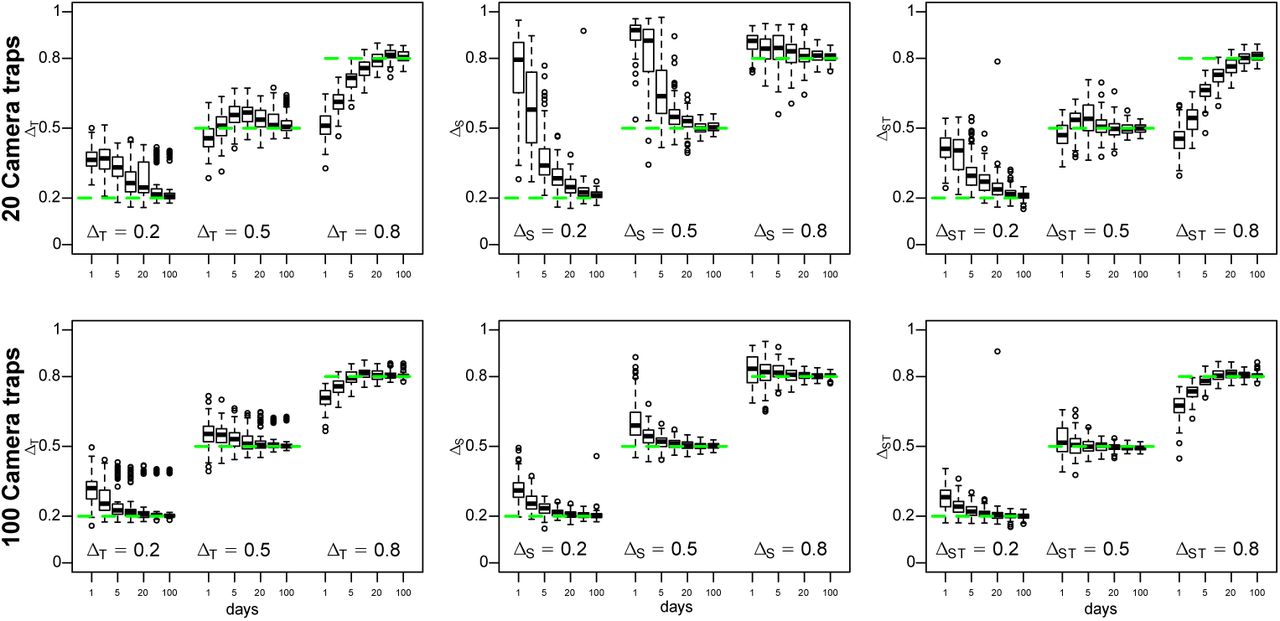
Distribution of bias in the estimated overlap coefficients  and
and  for different sample sizes.

Habitat preference of the three duiker species C. dorsalis, C. weynsi and S. grimmia. a) distribution of close canopy forest (CCF, top, green) and open woodland savanna (OSW, bottom, yellow) across the study region with the CNR borders and camera trap locations (black dots). b) Relative densities dsj of the three duikers predicted at 2,639 grid points. For each species the colors indicates  , where median
 is the median value over all the grid points j. Red shades indicate dsj > 0, blue shades dsj < 0. c) Posterior inclusion probabilities for the CCF (green) and OSW (yellow) habitat variables for each buffer. Values above the dashed line indicate the posterior probability that the habitat correlates positively with the relative species density, values below the dashed line imply a negative correlation.

Interaction in space and time between the duiker species C. dorsalis, C. weynsi, and S. grimma. Top row: interactions in space quantified as log10  between species 1 and 2. Bottom: posterior mean (solid line) and 90% credible intervals (shades) of temporal activity patterns. The area shaded in gray represents the overlap coefficient ΔT
The overlap measure Δ(f, g) can be related to the well known measure of distance between two densities L1 as
 which justifies the visualization of overlap coefficients between k species in a n-dimensional space using a Multidimensional Scaling (MDS) by considering
  as a measure of dissimilarity.
In practice, the true density functions f (x) and g(x) are usually not known. Here we obtain an estimate of Δ numerically from posterior samples. We distinguish three types of overlap coefficients, ΔT for overlap in time, ΔS for overlap in space and ΔST for overlap in time and space.
Overlap coefficient ΔT
For a large number nT of equally spaced time values  , we sample
  from the posterior distribution ℙ(ΔT |W(1), W(2)) where
  denotes the full data for a species l = 1, 2.
 where
where  is computed according to equation (5) with species specific parameters
  and
and  sampled from ℙ(θl|W (l)).
Overlap coefficient ΔS
For a given number nS of sites reflecting the habitat in a region, we sample  from the posterior distribution ℙ(ΔS |W (1), W (2)) as
 where
where  is computed according to equation (2) and normalized such as
  with species specific parameters
  and
and  sampled from ℙ(θl|W (l)).
Overlap coefficient ΔST
For nT time values and nS number of sites, we sample  from the posterior distribution ℙ(ΔST |W (1), W (2)) as
 where for species l = 1, 2 we calculate
  according to equation (5) and
  according to equation (2) with species specific parameters
  , and
, and  sampled from ℙ(θl|W (l)), but normalized such that

Implementation
All methods were implemented in the C++ program Tomcat, available through a git repository at https://bitbucket.org/WegmannLab/tomcat/.
3. Performance against simulations
We assessed the performance of our algorithm using 100 replicates for each combination of J = 20 or 100 camera trap locations and D = 1, 2, 5, 10, 20, 50 or 100 days at which data was collected. All simulations were conduced with one-dimensional Xj ∼ N (0, 1) and Yj ∼ N (0, 1) and parameter choices such that on average one picture per species per location was expected, and hence the expected number of pictures per species was JD.
To evaluate the accuracy of our estimates, we then estimated the overlap between two species since errors in parameter estimates directly translate into biases in overlap coefficients. We thus simulated data for two species with little (ΔT = 0.2), moderate overlap (ΔT = 0.5) or large overlap in time (ΔT = 0.8) as described in Table 1, as well as for two species with varying overlap in space (ΔS = 0.2, 0.5, and 0.8) and for with varying overlap in space and time (ΔST = 0.2, 0.5, and 0.8) as described in the Appendix.
Values of k used for the simulation of the daily activity patterns 𝒯 (t).
As shown in Figure 2, the posterior means  and
and  were unbiased and highly accurate for all overlap coefficients if sufficient data is provided, i.e. if at least several hundred pictures were available (J × D ≥ 500). If less data was available, estimates were biased towards the prior expectations of ΔT = 0.5 and ΔS = 1.
4. Application to central African duikers
We applied Tomcat to camera trapping data obtained during the dry seasons from 2012 to 2018 from a region in the Eastern Central African Republic (CAR), a wilderness exceeding 100000 km2 without permanent settlements, agriculture or commercial logging (Aebischer et al., 2017). The Eastern CAR consists of an ecotone of tropical moist closed canopy forests of the Northeastern Congolian lowland rain forest biome and a Sudanian-Guinean woodland savanna that is interspersed with small patches of edaphic grasslands on rocky ground or swampy areas (Boulvert, 1985; Olson and Dinerstein, 1998).
The available data was from 532 locations that cover the Chinko Nature Reserve (CNR), a protected area of about 20000 km2 that was established in 2014 by the government of the CAR in former hunting zones. Here, we use Tomcat to study duikers (Cephalophinae), which are a diverse mammalian group common in the data set and observed often in sympatry, i.e. several species were captured by the same camera trap within a few hours. We detected a total of eight species in the data set (Table 2): Cephalophus dorsalis castaneus (Eastern Bay Duiker), Cephalophus leucogaster arrhenii (Uele White Bellied Duiker), Cephalophus nigrifrons (Black Fronted Duiker), Cephalophus rufilatus (Red Flanked Duiker), Cephalophus silvicultor castaneus (Western Yellow Backed Duiker), Cephalophus weynsi (Weyns Duiker), Philantomba monticola aequatorialis (Eastern Blue Duiker) and Sylvicapra grimmia (Bush Duiker).
Available data on the eight detected species of duikers.
To infer habitat preferences for these species, we benefited from an existing land cover classification at a 30m resolution that represents the five major habitat types of the Chinko region: Closed Canopy Forest (CCF), Open Savanna Woodland (OSW), Dry Lakr Grassland (DLG), Wet Marshy Grassland (WMG) and Surface Water (SWA) (Aebischer et al., 2017). Around every camera trap location and 10,200 regular grid points spaced 2.5 km apart and spanning the entire CNR, we calculated the percentage of each of these habitats in 11 buffers of sizes 30, 65, 125, 180, 400, 565, 1260, 1785, 3,990, 5,640 and 17,840 meters. We complemented this information with the average value within every buffer for each of 15 additional environmental and bioclimatic variables from the WorldClim database version 2 (Table E.1 Fick and Hijmans, 2017) that we obtained at a resolution of 30 seconds, which translates into a spatial resolution of roughly 1km2 per grid cell. To aid in the interpretation, we then processed our environmental data by 1) keeping only the additional effect of each variables after regressing out the habitat variables CCF and OSW at the same buffer, and by 2) keeping only the additional effect of every variable after regressing out the information contained in the same variable but at smaller buffers (see Appendix for details).
To avoid extrapolation, we restricted our analyses to 2,639 grid locations that exhibited similar environments to those at which camera traps were placed as measured by the Mahanalobis distance between each grid point and the average across all camera trap locations (see Appendix for details).
For each location we further used the binary classification of the four most common habitat types (CCF, OSW, MWG, DLG) and determined the presence or absence of six additional habitat characteristics: Animal path, road, salt lick, mud hole, riverine zone and bonanza.
The eight duiker species varied greatly in both their habitat preferences (Figures 3, S.2) and their daily activity patterns (Figures 4, S.1) as inferred by Tomcat). As shown in Figure 3, C. dorsalis and C. weynsi have both a strong preference for CCF over OSW habitat at the smallest buffers, in contrast to S. grimmia that shows a string preference of OSW. At higher buffers, the signal is less clear, probably owing to the heterogeneous nature of the habitat in which both CCF and OSW correlated negatively with WMG and DLG, habitats not well suited for all these species. Interestingly, two species (P. monticola and C. silvicultor) also seem to be true ecotome species preferring a mixture of the canonical habitats CCF and OSW (Figure S.2). Similarly, and as shown in Figure 4, some species appear to be almost exclusively nocturnal (C. dorsalis and C. silvicultor), some almost exclusively diurnal (C. leucogaster, C. monticola, C. nigrifons, C. rufilatus, C. weynsi) and one crepuscular (S. grimmia).
To better understand how these closely related duiker species of similar size and nutrition can occur sympatrically, we estimated pairwise overlap coefficients in space and time (Figure 4, Table E.2). Not surprisingly, most species pairs differed substantially either in their habitat preference of daily activity patterns. Of the two forest dwellers C. dorsalis and C. weynsi  , for instance, one is almost exclusively nocturnal and the other almost exclusively diurnal
  , resulting in a small overlap in space and time
  . Similarly, the nocturnal C. dorsalis and the crepuscular S. grimmia that share a lot of temporal overlap
  use highly dissimilar habitats
  , resulting in a very small overlap in time and space
  .
.
A visualization using Multidimensional Scaling (MDS) of the pair-wise over-lap coefficients of all six species with events from at least 50 independent camera trap locations is shown in Figure 5. For these species, 88.3% of variation in the temporal overlap can be explained by a single axis separating nocturnal from diurnal species. In contrast, only 45.6% of the variation in the spatial overlap is explained by the first axis distinguishing forest dwellers from savanna species.
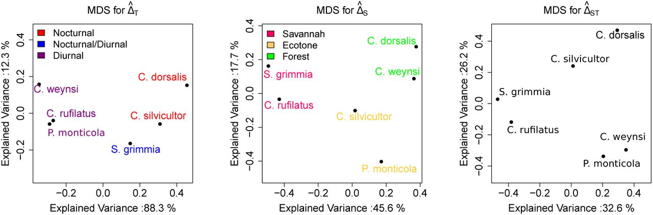
Illustration of the overlap coefficients in time and space between six duiker species visualized in two dimensions using the multidimensional scaling.
When using both temporal and spatial information, it is striking that frequently observed and therefore evidently abundant species within a certain community tend to differ in their habitat preference and/or daily activity. In contrast, infrequently observed and therefore putative rare taxa seem to have large overlap with co-occurring species. The Uele white-bellied duiker (C. leucogaster), for instance, which is rather rare and was only observed at eleven distinct locations (Table 2), depends on similar food and is active at the same time as the Weyns duiker (C. weynsi), which is among the most common forest duikers within the CNR. In contrast, the Eastern Bay duikers (C. dorsalis), which is strictly nocturnal, seems to co-exist with the Weyns duikers at higher densities (Figure (4).
Conclusion
Despite a world-effort to assess biodiversity, there are still major areas for which almost no information is available on biodiversity (e.g. Hickisch et al., 2019). But several technological advances, and in particular camera traps and voice recorders, make it possible to obtain a first glimpse on the presence and distribution of larger or highly vocal animals such as mammals and birds in relatively short time with a reasonable budget. Thanks to technical advances, increased battery life and larger media to store data, such data sets can now be produced with comparatively little manpower, even under the demanding conditions in large and remote areas. In addition, the annotation of such data sets on the species level is now aided by machine learning algorithms that automatize the detection of at least common species and images without animals (e.g. ?). Thanks to these developments, existing knowledge gaps may now be increasingly addressed, allowing for a re-evaluation of conservation strategies and optimization of conservation management.
Here we introduce Tomcat, a occupancy model that infers habitat preference and daily activities from such data sets. Unlike many previous methods that estimate the presence or absence of a species, Tomcat estimates relative species densities, from which overlap coefficients between species can be estimated in space and time, while accounting for variation in detection probabilities between locations. While estimates of overlap coefficients require larger data sets than the inference of pure occupancy, we believe they constitute a major step forward in understanding the complex species interactions in an area, which are particularly relevant for conservation planning in heterogeneous or fragmented habitat.
Appendix A. Simulating data with specific overlap coefficients
Simulating data with specific ΔS
For the simulation of scenarios with a given ΔS, we have simulated for each site j, an environmental variable Xj from N (0, 1). ΔS will be estimated with  , where
 where
where  in presence of n sites. For a species i and site
  is given by equation (2), with the constraint :
 We have for species 1 :

Equivalently, we have for species 2,  . Therefore,

We have
 We have
 The integral in equation (S.4) is given by:
 where Φ represents the cumulative distribution function (CDF) of the standard normal distribution.
Finally, we have
 It is possible using equation (S.5) to simulate a model for which ΔS = a.
For example, for ΔS = δs, and for A1 = a1, it is possible to get the value of A2 from (S.5), which gives
 After computing A2, it is easy to deduce the value of µ2 using equation (S.2).
Simulating data with specific ΔST
To simulate scenarios for a given ΔST, we have simulated for each site j an environmental variable Xj from N (0, 1), and T ∼ U[0,24]. ΔST is estimated using equation (11).
For a species i and site j, we have the constraint
 where 𝒯i(t) is the daily activity for a species i, i = 1, 2 observed at time t.
We have
 and
and
 which gives
 We can therefore simulate the scenario ΔST = δST with known activity patterns 𝒯1, 𝒯2 respectively for species 1 and 2 as follows:
Simulate ns Xj ∼ N (0, 1), j = 1, 2, …ns.
Propose a value of A1. (Should not be very large. Namely between −2 and 2).
Compute the value of µ1 using equations (S.7).
Compute numerically the value of A2 by solving the equation :

Using Tomcat for the two species, and by fixing the value Ai, i = 1, 2, we can sample from the posterior distribution of ΔST and compute the posterior mean of the values ΔST using equation (11).

Appendix B. Decorrelation environmental variables
While Tomcat readily handles correlated environmental variables, we chose to decorrelate specific variables to aid in interpretation. Specifically, we processed our environmental data as follow (two steps):
Step 1: A major interest in our application was to study the impact of the prevalence of close canopy forest (f) and savanna (s) habitat on species densities. For each scale (buffer) b, we therefore regress each environmental variable Vib, i ≠ f, s:
 where Vfb and Vsb represents, respectively, the forest and the Savannah habitat for a buffer b = 1, …, B, i = 1, …, nenv, and ϵib is the error from the linear model described by equation (S.1), which captures the information of the variable Vib independent of Vfb and Vsb at buffer b. We therefore replace the Vib variables by
  in our model, but kept
  and
and  .
.
Step 2: To evaluate relevant spatial scale of environmental variables, we also regressed out the larger buffers from the smaller one as:
 In the second step, and for a given environmental variable
  at the scale, we give priority to the smaller scales by keeping only the additional explanation by the studied variable to what we already know by replacing
  by
by  .
.
Appendix C. Restricting analysis to environmentally homogeneous regions
Let  be a matrix where the rows represent the observed camera traps, and the columns the environmental variables, and let
  a matrix containing the environmental variables for the locations for which we want to predict
  .
.
We define the Mahanalobis distance DO of  given by
 where
where  , and S is the variance covariance matrix.
We define a second Mahalanobis distance DP which measures the distance of  from the the mean
  of the camera traps environmental variables. DP is given by
 After computing DO and DP, we decided to remove the grid points for which we have DP > 1.2 × max(DO).
Appendix D. Supplementary figures

Estimation of the daily activity of the 8 observed duickers. The solid line represents the posterior mean and the shades, 90% credible intervals of the temporal activity patterns.

Relative densities dsj of the eight duikers predicted at 2,639 grid points. For each species the colors indicates  , where median
  is the median value over all the grid points j. Red shades indicate dsj > 0, blue shades dsj < 0.
Appendix E. Supplementary tables
Environmental and bioclimatic variables obtained from the WorldClim database version 2.
Summary of the overlap coefficients between the six duiker species.


