

Abstract
Spiral fMRI has been put forward as a viable alternative to rectilinear echo-planar imaging, in particular due to its enhanced average k-space speed and thus high acquisition efficiency. This renders spirals attractive for contemporary fMRI applications that require high spatiotemporal resolution, such as laminar or columnar fMRI. However, in practice, spiral fMRI is typically hampered by its reduced robustness and ensuing blurring artifacts, which arise from imperfections in both static and dynamic magnetic fields.
Recently, these limitations have been overcome by the concerted application of an expanded signal model that accounts for such field imperfections, and its inversion by iterative image reconstruction. In the challenging ultra-high field environment of 7 Tesla, where field inhomogeneity effects are aggravated, both multi-shot and single-shot 2D spiral imaging at sub-millimeter resolution was demonstrated with high depiction quality and anatomical congruency.
In this work, we further these advances towards a time series application of spiral readouts, namely, single-shot spiral BOLD fMRI at 0.8 mm in-plane resolution. We demonstrate that spiral fMRI at 7 T is not only feasible, but delivers both competitive image quality and BOLD sensitivity, with a spatial specificity of the activation maps that is not compromised by artifactual blurring. Furthermore, we show the versatility of the approach with a combined in/out spiral readout at a more typical resolution (1.5 mm), where the high acquisition efficiency allows to acquire two images per shot for improved sensitivity by echo combination.
Highlights
This work reports the first fMRI study at 7T with spiral readout gradient waveforms.
We achieve spiral fMRI with sub-millimeter resolution (0.8 mm, in-plane FOV 230 mm), acquired in a single shot.
Spiral images exhibit intrinsic geometric congruency to anatomical scans, and spatially highly specific activation patterns.
Image reconstruction rests on a signal model expanded by measured trajectories and static field maps, inverted by cg-SENSE.
We assess generalizability of the approach for spiral in/out readouts, providing two images per shot (1.5 mm resolution).
1 Introduction
Functional MRI (fMRI) is presently the most prominent technique to study human brain function non-invasively, owing to its favorable spatiotemporal resolution regime with appealing functional sensitivity. Within this regime, specific research questions require different trade-offs between spatial and temporal resolution. On the one hand, ultra-high spatial resolution fMRI at sub-millimeter voxel size successfully targets smaller organizational structures of the brain, such as cortical laminae (Fracasso et al., 2016; Huber et al., 2017a; Kashyap et al., 2018; Kok et al., 2016; Lawrence et al., 2018; Martino et al., 2015; Muckli et al., 2015; Siero et al., 2011) and columns (Cheng et al., 2001; Feinberg et al., 2018; Yacoub et al., 2008), or subcortical nuclei, but requires compromises on coverage (FOV) or temporal bandwidth, i.e., volume repetition time (TR). On the other hand, fast sequences with TRs on the order of 0.5 seconds and below are important for advanced analysis approaches, e.g., to adequately sample physiological fluctuations (Lewis et al., 2016; Smith et al., 2013; Uğurbil et al., 2013), at the expense of lowering spatial resolution (2–4 mm).
One means to simultaneously advance the spatial and temporal resolution boundaries of fMRI is to maximize acquisition efficiency, i.e., sampled k-space area (or volume) per unit time. Therefore, fMRI nowadays almost exclusively relies on rectilinear echo-planar imaging (EPI, (Cohen and Schmitt, 2012; Mansfield, 1977; Schmitt et al., 2012)), where acquisition efficiency is favorable due to optimal acceleration and high terminal velocity along the straight k-space lines traversed.
To expand spatiotemporal resolution beyond the capabilities of EPI alone, the main strategy has been parallel imaging acceleration (Griswold et al., 2002; Pruessmann et al., 1999), in combination with simultaneous multi-slice or 3D excitation (Breuer et al., 2006; Larkman et al., 2001; Poser et al., 2010; Setsompop et al., 2012). In terms of k-space coverage per unit time, the benefit of parallel imaging lies in expanding the cross section of what is effectively a tube of k-space covered along the readout trajectory (Pruessmann, 2006). By focusing efforts on maximizing acquisition efficiency in this way, another key determinant of the speed of coverage was less emphasized, which is the average velocity along the trajectory, i.e., the average instantaneous gradient strength. On this count, EPI is wasteful because it includes many sharp turns that must be traversed at low speed because of limited gradient slew rate.
It has long been recognized, also in the context of fMRI (Barth et al., 1999; Glover, 2012; Noll et al., 1995), that substantially higher average k-space speed and thus acquisition efficiency is achieved with spiral trajectories, which avoid sharp turns by distributing curvature more evenly (Ahn et al., 1986; Likes, 1981; Meyer et al., 1992). Typically, single-shot variants winding out of k-space center, e.g., on an Archimedean spiral, are prevalent (Glover, 1999; Meyer et al., 1992), but different acquisition schemes, such as spiral-in (Börnert et al., 2000) or combined in/out readouts (Glover and Law, 2001; Glover and Thomason, 2004) have been proposed. High resolution fMRI studies have occasionally employed spirals as well (Jung et al., 2013; Singh et al., 2018), albeit reducing acquisition efficiency in favor of robustness by acquiring k-space in multiple shots with shorter spiral readouts.
However, routine use of spiral fMRI has not been established, due to the following three challenges (Block and Frahm, 2005; Börnert et al., 1999): First, spirals are sensitive to imperfect magnetic field dynamics (eddy currents and other gradient imperfections, as well as subject-induced field changes, e.g., via breathing) which lead to blurring and image distortions. Secondly, non-uniformity of the static Bo field, caused by varying susceptibility of the imaged tissues, likewise causes blurring. Finally, in combination with parallel imaging, spirals pose a somewhat greater reconstruction challenge than Cartesian trajectories (Pruessmann et al., 2001).
Recently, these obstacles have been overcome (Engel et al., 2018b; Kasper et al., 2018; Wilm et al., 2017) by (1) employing an expanded signal model that accounts for the actual static and dynamic fields as well as coil sensitivity encoding (Wilm et al., 2011), and (2) the inversion of this model by an accompanying iterative image reconstruction (Barmet et al., 2005; Man et al., 1997; Pruessmann et al., 2001; Sutton et al., 2003). This approach enabled the use of very long spiral readouts (on the order of 50 ms at 7 Tesla), while maintaining competitive image quality and anatomical fidelity. In particular, such enhanced spiral acquisition efficiency was demonstrated by accomplishing T2*-weighted images with an in-plane resolution of 0.8 mm in a single shot. Ultimately, these findings hold promise that spiral fMRI can now indeed profit from the theoretical advantages of enhanced acquisition efficiency to expand the spatiotemporal boundaries of fMRI.
Based on these advances in expanded signal modeling and inversion, in this work, we explore the feasibility and utility of sub-millimeter single-shot spiral fMRI. Specifically, we first assess image quality and temporal stability of fMRI time series obtained with the expanded signal model and algebraic reconstruction. We further evaluate the resulting functional sensitivity, using an established visual quarter-field stimulation to elicit reference activation patterns and demonstrate spatial specificity and geometric consistency of the resulting activation at the level of the nominal resolution (0.8 mm). Finally, we explore the versatility of the approach with a combined in/out spiral readout at a more typical resolution (1.5 mm). Here, two images per shot can be acquired, translating the high acquisition efficiency of the spiral into enhanced functional sensitivity by echo combination (Glover and Law, 2001; Glover and Thomason, 2004; Law and Glover, 2009).
2 Methods
2.1 Setup
All data was acquired on a Philips Achieva 7 Tesla MR System (Philips Healthcare, Best, The Netherlands), with a quadrature transmit coil and 32-channel head receive array (Nova Medical, Wilmington, MA).
Concurrent magnetic field monitoring was performed using 16 fluorine-based NMR field probes, which were integrated into the head setup via a laser-sintered nylon frame positioned between transmit and receive coil (Engel et al., 2018b, Fig. 1). Probe data were recorded and preprocessed (filtering, demodulation) on a dedicated acquisition system (Dietrich et al., 2016a). The final extraction of probe phase evolution and projection onto a spherical harmonic basis set (Barmet et al., 2008) was performed on a PC, yielding readout time courses of global phase k0 and k-space coefficients kx, ky, kz with 1 MHz bandwidth.

Utilized 2D single-shot spiral acquisitions (R=4 undersampling): High-resolution single-shot spiral-out (nominal resolution 0.8 mm, black) and spiral in/out trajectory (1.5 mm resolution, blue). Depicted are the gradient waveforms (Gx,Gy,Gz) as well as RF excitation (Tx) and ADC sampling interval s (AQ) for both the 1H head coil and the 19F field probes used to monitor the trajectories and other concurrent encoding fields. Field probe excitation and acquisition start a few milliseconds before the spiral readout gradient waveforms.
For the fMRI experiments, visual stimulus presentation utilized VisuaStim LCD goggles (Resonance Technology Inc., Northridge, CA, USA). A vendor-specific respiratory bellows and finger pulse plethysmograph recorded subject physiology, i.e., respiratory and cardiac cycle.
2.2 fMRI Paradigm and Subjects
Seven healthy subjects (4 female, mean age 25.7 +/-4.1 y) took part in this study, after written informed consent and with approval of the local ethics committee. One subject was excluded from further analysis due to reduced signal in multiple channels of the head receive array. Thus, six subjects were analyzed for this study.
The paradigm, a modified version of the one used in (Kasper et al., 2014), comprised two blocks of 15 s duration that presented flickering checkerboard wedges in complementary pairs of the visual quarter-fields. In one block, upper left and lower right visual field were stimulated simultaneously (condition ULLR), while the other block presented the wedges in the upper right and lower left quarter-fields (condition URLL). These stimulation blocks were interleaved with equally long fixation periods. To keep subjects engaged, they had to respond to slight contrast changes in the central fixation cross via button presses of the right hand. A single run of the paradigm took 5 min (5 repetitions of the ULLR-Fixation-URLL-Fixation sequence).
2.3 Spiral Trajectories and Sequence Timing
Spiral fMRI was based on a slice-selective multi-slice 2D gradient echo sequence (Fig. 1) with custom-designed spiral readout gradient waveforms. For every third slice, concurrent field recordings were performed on the dedicated acquisition system (Dietrich et al., 2016a), with NMR field probes being excited a few milliseconds prior to readout gradient onset (Fig. 1, bottom row, (Engel et al., 2018b)).
For the spiral trajectories, we selected two variants that had previously provided high-quality images in individual frames (Engel et al., 2018b, Fig. 2): a high-resolution case winding out of k-space center on an Archimedean spiral (spiral-out, Fig. 1, black gradient waveform), and a combined dual-image readout first spiraling into k-space center, immediately followed by a point-symmetric outward spiral (spiral in/out (Glover and Law, 2001)), Fig. 1, blue gradient waveform).

Overview of image quality for high-resolution (0.8 mm) single-shot spiral-out acquisition. (A) 8 oblique-transverse slices (of 36) depicting the time-series magnitude mean of one functional run (subject S7, 100 volumes). (B) Single-volume magnitude images for slices corresponding to lower row of (A). (C) Mean phase image over one run, without any post-processing, for slices corresponding to lower row of (A).
The spiral-out gradient waveform was designed to deliver the highest spatial resolution possible under several constraints. First, targeting maximum acquisition efficiency in 2D commands a single-shot 2D readout, because the sequence overhead, i.e., time spent without sampling k-space, accrues for each new excitation. Second, the parallel imaging capability of our receiver array at 7 T allowed for an in-plane acceleration factor of R=4 (determining the spacing of the spiral revolutions, i.e., FOV). We based this choice on previous experience with spirals of such undersampling using this setup (Engel et al., 2018b; Kasper et al., 2018), which were free of aliasing artifacts or disproportional noise amplification. Third, the requirement of concurrent field recordings for the whole spiral readout limited its maximum duration to below 60 ms. This is the approximate lifetime of the NMR field probe signal, after which complete dephasing occurs in a subset of probes for this specific setup, governed by their T2* decay time of 24 ms (Engel et al., 2018b). Finally, the gradient system specifications constrain the maximum possible resolution (or k-space excursion) of an Archimedean spiral with prescribed FOV and duration. Here, we used the optimal control algorithm by (Lustig et al., 2008) to design time-optimal spiral gradient waveforms of 31 mT/m maximum available gradient amplitude, and a 160 mT/m/ms slew rate limit, chosen for reduced peripheral nerve stimulation.
Overall, these requirements led to a spiral-out trajectory with a nominal in-plane resolution of 0.8 mm (for a FOV of 230 mm), at a total readout acquisition time (TAQ) of 57 ms. BOLD-weighting was accomplished by shifting the readout start, i.e., TE, to 20 ms.
For the spiral in/out, we followed the same design principles, targeting a minimum dead time after excitation, and a symmetric readout centered on a TE of 25 ms, slightly shorter than reported T2* values in cortex at 7 T (Peters et al., 2007). This resulted in a gradient waveform lasting 39 ms, with a nominal resolution of 1.5 mm for each half-shot of the trajectory.
All other parameters of both spiral sequences were shared, in order to facilitate comparison of their functional sensitivity. In particular, slice thickness (0.9 mm) and gap (0.1 mm) were selected for near-isotropic sub-mm resolution for the spiral-out case, while still covering most of visual cortex. For each slice, the imaging part of the sequence (Fig. 1) was preceded by a fat suppression module utilizing Spectral Presaturation with Inversion Recovery (SPIR, (Kaldoudi et al., 1993)).
The sequence duration totaled 90 ms per slice for the spiral-out sequence (TE 20 ms + TAQ 60 ms + SPIR 10 ms), which was maintained for the spiral in/out, even though a shorter imaging module would have been possible. To arrive at a typical volume repetition time for fMRI, we chose to acquire 36 slices (TR 3.3 s). Each functional run comprised 100 volume repetitions, amounting to a scan duration of 5.5 min.
2.4 Image Reconstruction
Image reconstruction rested on an expanded model of the coil signal sγ (Wilm et al., 2011), that – besides transverse magnetization m – incorporates coil sensitivity cγ, as well as phase accrual by both magnetostatic Bo field inhomogeneity (offresonance frequency Δω0) (Barmet et al., 2005) and magnetic field dynamics kl expanded in different spatial basis functions bl (Barmet et al., 2008):
 with coil index γ, sampling time t, imaging volume V, and location vecto r = [x y z]T
For 2D spiral imaging without strong higher order eddy currents (e.g., as induced by diffusion encoding gradients), this model can be computationally reduced (Engel et al., 2018b) to facilitate iterative inversion. To this end, we (1) considered only field dynamics contributing to global phase k0 and spatially linear phase, i.e., k-space k = [kx ky kz], as provided by the concurrent field recordings, and (2) restricted the integration to the excited 2D imaging plane by shifting the coordinate origin to the slice center r0, effectively factoring slice-orthogonal field dynamics out of the integral:
 For the demodulated coil signal
  , the discretized version of eq. (2) – respecting finite spatial resolution and dwell time of the acquisition system – reads as a system of linear equations
 with sampling time index τ, voxel index
  , encoding matrix element
  , and
, and  .
.
The matrix-vector form of eq. (3) is a general linear model,
 and can be efficiently solved iteratively by a conjugate gradient (CG) algorithm (Pruessmann et al., 2001; Shewchuk, 1994). As mentioned above, the restriction to first order field dynamics enables acceleration of the ensuing matrix-vector multiplications by (reverse) gridding and fast Fourier transform (FFT) (Beatty et al., 2005; Jackson et al., 1991). Offresonance effects can also be approximated by FFT using multi-frequency interpolation (Man et al., 1997).
This image reconstruction algorithm was applied equivalently to the spiral-out and spiral in/out data. Note, however, that for the latter both field recordings and coil data were split into their in- and out-part and reconstructed separately, yielding two images per shot.
Taken together, the in-house Matlab (The Mathworks, Natick, MA, R2018a) implementation of this algorithm led to reconstruction times of about 10 min per slice on a single CPU core. In order to reconstruct the 3600 2D images per fMRI run, reconstruction was parallelized over slices on the university’s CPU cluster. Depending on cluster load, reconstructions typically finished over night for the high-resolution spiral out, and within 2 h for the spiral in/out data.
The auxiliary input data for the expanded signal model, i.e., spatial maps for static Bo field inhomogeneity Δω and coil sensitivity cγ, were derived from a separate fully sampled multi-echo (ME) Cartesian gradient echo reference scan of 1 mm in-plane resolution, TE1 = 4ms, ΔTE = 1ms (Kasper et al., 2018), with slice geometry equivalent to the spiral sequences. Image reconstruction proceeded as described above for this scan, albeit omitting the sensitivity and static Bo map terms. The latter was justified by the high bandwidth of the Cartesian spin-warp scans (1 kHz).
Sensitivity maps were then computed from the first-echo image, normalizing single coil images by the root sum of squares over all channels, while the Bo map was calculated by regressing the pixel-wise phase evolution over echo images. Both maps were smoothed and slightly extrapolated via a variational approach (Keeling and Bammer, 2004).
2.5 Data Analysis
2.5.1 Image Quality Assessment
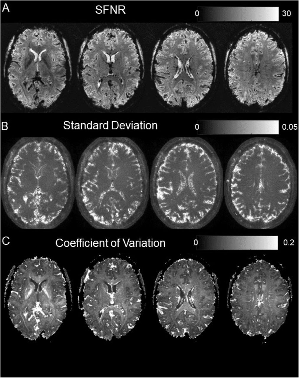
The suitability of the raw imaging data for high-resolution fMRI was assessed in terms of both sensitivity and spatial specificity. For sensitivity, we evaluated the temporal statistics of the images, i.e., signal-to-fluctuation noise ratio (SFNR), standard deviation (SD) and coefficient of variation (CoV) maps (Welvaert and Rosseel, 2013), defined as
 where the bar denotes averaging over volumes of a run.
For spatial specificity, we visually compared the spiral images to the ME reference scan, which exhibits a high geometric veracity due to its spin-warp nature, i.e., high bandwidth. We overlaid the contour edges (intensity isolines) of the mean (over echoes) of the ME images onto the mean spiral images  to inspect the congruency of anatomical boundaries between the scans.
To reduce the impact of subject motion on both assessments, the volumes of the fMRI time series were first realigned to each other. Then, the mean ME scan was co-registered to the resulting mean realigned fMRI scan, Importantly, both operations were limited to six-parameter rigid-body registration, such that nonlinear geometric distortions between sequences were not corrected through this preprocessing step. Furthermore, to facilitate visual comparison and contour edge creation, mean ME and spiral images were bias-field corrected using unified segmentation (Ashburner and Friston, 2005).
All computations were performed in Matlab R2018b, using the Unified NeuroImaging Quality Control Toolbox (UniQC, (Bollmann et al., 2018)), and SPM12 (Wellcome Centre for Human Neuroimaging, London, UK, http://www.fil.ion.ucl.ac.uk/spm/).
2.5.2 BOLD fMRI Analysis
The main goal of this analysis was to establish the functional sensitivity of the spiral fMRI sequences at the single-subject level under standard paradigm and preprocessing choices. On a qualitative level, we also assessed the spatial specificity of functional activation.
Equivalent preprocessing steps were applied to all spiral fMRI runs using SPM12. After slice-timing correction, we employed the pipeline described in the previous section (realignment, co-registration, bias-field correction via unified segmentation). Finally, the functional images were slightly smoothed with a Gaussian kernel of 0.8mm FWHM, i.e., the voxel size of the high-resolution scan.
The general linear model (GLM) contained regressors of the two stimulation blocks (ULLR and URLL) convolved with the hemodynamic response function (HRF), as well as nuisance regressors for motion (6 rigid-body parameters) and physiological noise (18 RETROICOR (Glover et al., 2000) regressors, as specified in (Harvey et al., 2008)), extracted by the PhysIO Toolbox (Kasper et al., 2017).
To characterize functional sensitivity, we evaluated the differential t-contrasts +/-(ULLR-URLL) and report results both with and without multiple comparison correction. For visualization, Figures 5–7 show activations without correction, at a threshold of p<0.001 (t>3.22). This helps to demonstrate the spatial specificity of activations. By contrast, Table 1 reports activations under whole-brain family-wise error (FWE) correction at the cluster level (p<0.05), with a cluster defining threshold (p<0.001) that corresponds to the threshold used for visualization.
Quantification of temporal stability and functional sensitivity of all spiral fMRI sequences. For the signal-to-fluctuation-noise ratio (SFNR, eq. (5)), the table contains mean +/-SD in a gray matter ROI over the whole imaging volume. For the t-contrast SPMs, peak t-value and number of significant voxels over both differential contrasts (+/-ULLR-URLL) are reported (p<0.05 FWE-corrected for multiple comparisons at the cluster level with a cluster-forming threshold of 0.001). The last column shows relative increases to the previous sequence, i.e., the one reported in the sub-table directly above. Since resolutions differ between spiral-out (0.8 mm) and spiral in/out (1.5 mm), we compare activated volume instead of voxel count.
Spatial specificity of the activation was qualitatively assessed by overlaying the thresholded t-contrast maps for both contrasts onto the anatomically veridical mean ME image. We checked whether activation patterns were restricted to gray matter regions of visual cortex, as well as whether the spatial separation and symmetry of activations were linked to distinct quarter-field stimulation patterns, as expected by the retinotopic organization of visual cortex (Engel et al., 1997; Wandell et al., 2007; Warnking et al., 2002). On top, we also evaluated the individual contrasts for the ULLR and URLL stimulation blocks to assess the spatial overlap of their activation patterns as an alternative measure of functional specificity (since the differential contrasts cannot overlap by design).
This overall analysis procedure was performed for the spiral-out as well as the individual spiral-in and spiral-out image time series reconstructed from the spiral in/out data. As spiral in/out sequences are predominantly selected for their potential gain in functional sensitivity when combining spiral-in and spiral-out images (Glover and Law, 2001), we additionally repeated the BOLD fMRI analysis for such a surrogate dataset (“in/out combined”). We chose a signal-weighted combination per voxel (Glover and Thomason, 2004), which is considered the most practical approach for echo combination (Glover, 2012):
 with m1 and m2 being the in-part and out-part voxel time series, respectively.
2.6 Code and Data Availability
Image reconstruction was performed by an in-house custom Matlab implementation of the cg-SENSE algorithm (Pruessmann et al., 2001). A demonstration of that algorithm is publicly available on GitHub (https://github.com/mrtm-zurich/rrsg-arbitrary-sense), with a static compute capsule for reproducible online re-execution on CodeOcean (Patzig et al., 2019), which were created in the context of the ISMRM reproducible research study group challenge (Stikov et al., 2019), albeit without the multi-frequency interpolation employed here.
Image and fMRI analyses were performed using SPM12 (https://www.fil.ion.ucl.ac.uk/spm distributed under GPLv2) and the UniQC Toolbox. UniQC is developed in-house, and a beta-version can be downloaded from the Centre for Advanced Imaging software repository on GitHub (https://github.com/CAIsr/uniQC); a publicly available stable release will be made available in 2020 as part of the TAPAS Software Suite (http://translationalneuromodeling.org/tapas), under a GPLv3 license.
All custom analysis and data visualization scripts will be available on http://github.com/mrikasper/paper-advances-in-spiral-fmri. This includes both a one-click analysis (main.m) to rerun all image statistics and fMRI analyses, as well as the automatic re-creation of all figure components found in this manuscript (main_create_figures.m), utilizing the UniQC Toolbox. More details on installation and execution of the code can be found in the README.md file in the main folder of the repository.
One dataset from this study (SPIFI_0007) will be made publicly available on ETH Research Collection, upon acceptance of this paper, according to the FAIR (Findable, Accessible, Interoperable, and Re-usable) data principles (Wilkinson et al., 2016). This includes both the reconstructed images in NIFTI format with BIDS metadata, to validate the analysis scripts, as well as raw coil and trajectory data in ISMRMRD format. For the other datasets, we did not obtain explicit subject consent to share all raw data in the public domain. However, we do provide the mean spiral fMRI images with corresponding activation t-maps for all subjects on NeuroVault ((Gorgolewski et al., 2015), https://neurovault.org/collections/6086/).
3 Results
3.1 Spiral Image Quality, Congruency and Stability
In the following, we mainly present images from two subjects (S7: Figs. 2,3, S2: Figs. 4,5,7). However, as illustrated by Fig. 6, results were comparable for all six analyzed datasets. In addition to Fig. 6, this can be inspected in the supplementary material (Fig. S1) or on NeuroVault ((Gorgolewski et al., 2015), https://neurovault.org/collections/6086/).
The mean images (one run of subject S7, after realignment) of the high-resolution spiral-out sequence exhibit good image quality, rich in T2* contrast and anatomical detail (Fig. 2A). In the center of the brain, no blurring is apparent, and anatomical boundaries can be clearly delineated, e.g, the optic radiation, down to the single-voxel extent. Moderate residual imaging artifacts (local ringing, blurring) are visible in the orbitofrontal areas, at some brain/skull boundaries, and in the vicinity of larger muscles and fat deposits, e.g., the temporal muscles. For more inferior slices, signal dropouts can be identified at typical sites of through-plane dephasing, e.g., above the ear canals. Individual frames of the time series exhibit similar features (Fig. 2B), though somewhat noisier, as expected because of the reduced SNR.
Interestingly, the mean of the corresponding raw phase images also contains high anatomical detail and few phase wraps (Fig. 2C), which are again located at the interface between brain and skull or close to air cavities. Note that the unwrapped appearance of the phase image is a feature of the Bo-map based correction (Kasper et al., 2018) and does not require any postprocessing.
Mapping the temporal statistics of the spiral image time series (Fig. 3, Table 1) proves its sufficient stability for functional imaging in all slices. The SFNR images (Fig. 3A) are rather homogeneous, with mean values of 15.3 +/-1.1 in cortical gray matter, averaged over subjects (Table 1). A slight reduction for central brain regions is visible due to the diminished net sensitivity of the receiver array. Notably, no structured noise amplification through bad conditioning of the undersampled reconstruction problem (g-factor penalty) is discernible in this area.

Characterization of image time series fluctuations over 1 spiral-out run (95 volumes, discarding first five). (A) Signal-to-Noise Fluctuation Ratio (SFNR) image for same slices as in Fig 2. Rather homogeneous, exhibiting sufficient SFNR levels. (B) Standard deviation (SD) image over time. Regions of high fluctuation mainly include pulsatile areas close to ventricles or major blood vessels, and cortex/CSF interfaces. (C) Coefficient of Variation (CoV) image. Inverse of (A), highlighting regions of high fluctuations relative to their respective mean. Vascularized/CSF regions appear prominently, as well as the internal capsule, due to its reduced average signal level.
The SD images (Fig. 3B) corroborate this impression, showing peak values in ventricles (CSF) and highly vascularized areas (insula, ACC). These noise clusters presumably stem from fluctuations through cardiac pulsation and are not specific to spiral acquisitions. However, for the raised SD values in voxels close to the cortex borders, it is unclear whether also CSF fluctuations, the BOLD effect itself, or rather time-varying blurring due to unaccounted magnetic field fluctuations contribute. This is scrutinized in the GLM analysis below. Additionally, for the CoV images (Fig. 3C), the internal capsule appears prominently, presumably due to its reduced average signal level.
In terms of spatial specificity, overlaying contour edges of the anatomical reference (mean ME spin-warp image, subject S2) (Fig. 4A,E) onto the mean spiral-out image suggests a geometrically very faithful depiction of the anatomical interfaces (Fig. 4B,F). Boundaries of the ventricles and cortex to white matter are congruent in general, also for the visual areas considered in later analyses, and are not blurry. Some regions of the spiral-out images suffer from ringing (yellow arrow) or signal dropout (white arrow), most likely due to through-plane dephasing and incomplete in-plane Bo correction.
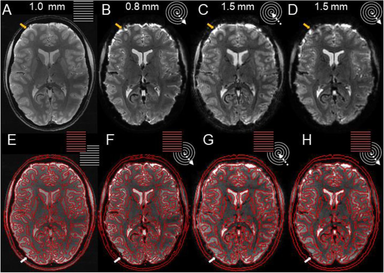
Image quality and geometric accuracy of spiral images, reconstructed with the expanded signal model. (A) Anatomical Reference: Mean multi-echo (ME) spin-warp image (1 mm resolution) (B) High-resolution (0.8 mm) spiral-out; (C) In-part of spiral in/out (1.5 mm); (D) Out-part of spiral in/out (1.5 mm). (E-H) Overlay of isoline contour edges from (A) onto (A)-(D).
Depicted are the mean images of a single run (subject S2, top row, B-D). The mean ME image (A), used to compute SENSE- and B0-map for the expanded signal model, provides the anatomical reference via its contours (E, red lines). These are overlaid onto the different spiral variants (bottom row, F-H). Arrows indicate residual geometric incongruence by through-plane dephasing (white) or incomplete Bo mapping and correction (yellow) in the spiral-out, which are reduced in the out-part and absent in the in-part of the spiral-in/out sequence.
Incorporating the mean images of the spiral in/out sequence into the comparison confirms the nature of these artifacts (Fig. 4C,D,G,H). The in-part images (Fig. 4C) are void of these artifacts and match the anatomical reference almost completely in terms of edge contours (Fig. 4G). Only CSF/skull interfaces are slightly compromised by a more global ringing, presumably from residual fat or high-intensity signal right after slice excitation. The out-part of the spiral-in/out (Fig. 4D,H) constitutes a compromise between spiral-in and high-resolution spiral-out in terms of artifact-level. Its shorter readout of only 20 instead of 60 ms alleviates through-plane dephasing or incomplete Bo correction through inaccurate mapping.
3.2 Functional Sensitivity and Specificity
Functional sensitivity of the high-resolution spiral-out images is evident at the single-subject level (subject S2) in a differential contrast of both stimulus conditions (+/-ULLR-URLL). The corresponding t-map, overlaid on the mean functional images, reveals expected activation patterns in visual cortex (Fig. 5A). Hemispheric separation of the complementary quarter-field stimulation blocks is visible (left slice), as well as the contrast inversion from inferior to superior slices (left vs second left slice). Notably, significant activation flips between neighboring voxels occur at the cerebral fissure, suggesting spatial specificity at the voxel level.

Visual Activation Maps of high-resolution (0.8 mm) spiral-out fMRI for a single subject (S2). Representative stimuli of both conditions (ULLR and URLL) are displayed at the top. (A) Overlay of differential t-contrast maps (p<0.001 uncorrected) on transverse slices of mean spiral image (hot colormap: URLL-ULLR, cool colormap: ULLR-URLL). (B) Same contrast maps as in (A), overlaid on mean ME image as anatomical reference. (C) Zoomed-in sections of differential t-contrast maps in different orientations: transverse (top), coronal (middle) and sagittal (bottom, left (L) and right (R) hemisphere). (D) t-contrast maps for individual conditions (blue: ULLR, yellow: URLL), showing more widespread activation and high spatial specificity, i.e., little spatial overlap (green).
This functional specificity is confirmed when overlaying the identical activation maps on the mean ME image as anatomical reference (Fig. 5B), again demonstrating the good alignment of functional and structural data seen in the previous subsection (Fig. 4). Clustered activation is almost exclusively constrained to gray matter with no extension into adjacent tissue or skull. Note that no multiple comparison correction was performed for visualization, in order to be more sensitive to such effects, at the expense of occasional false-positive voxels throughout other brain areas.
Gray-matter containment and retinotopic organization of the activation can be further corroborated in the zoomed-in sections of visual cortex for transverse, coronal and sagittal orientation (Fig. 5C). Additionally, we evaluated the ULLR and URLL blocks individually (Fig. 5D), because differential contrasts, by design, do not allow for spatial overlap between significant activation of both conditions. In the individual contrasts, the identified portion of activated visual cortex appears larger, but is still very well restricted to cortical gray matter. Few overlaps exist, and, again, contrast switches between adjacent voxels, pointing to spatial specificity at the prescribed sub-mm resolution.
These findings are reproducible over subjects (Fig. 6). Importantly, similar image quality and geometric congruency are accomplished in all subjects. To verify, we show both the mean spiral and the anatomical ME reference image of the corresponding transverse slice as underlays for the differential activation patterns. Some subjects exhibit more frontal blurring artifacts and dropouts (S5, S6, S7) due to different geometry of the air cavities. Still, the retinotopic organization of visual cortex is recovered in all subjects, as visualized in the zoomed coronal and sagittal views. Existing differences of the specific activation patterns are within the expected range of variability in subject anatomy and task engagement. Quantitatively, peak t-values reach 15.1 on average for the differential contrasts, with a standard deviation of 2.6, i.e. 17 %, over subjects (Table 1). Activation clusters comprise 10371 +/-2480 voxels (after FWE-multiple comparison correction at the cluster level, p<0.05), i.e., 6467 +/-1547 mm3.

Mean spiral images and activation maps over subjects (S2-S7) for high-resolution spiral-out fMRI. For each subject, the following 4 sections are displayed, with the mean ME image as anatomical underlay: transverse, coronal and sagittal slice (for left (L) and right (R) hemisphere), each chosen for the maximum number of activated voxels (over both differential statistical t-contrasts, p<0.001 uncorrected). To assess raw spiral data quality, the corresponding mean functional image is displayed side-by-side to the anatomical transverse slice as an alternative underlay.
3.3 Spiral In/Out Analysis and Echo Combination
We continue to present data from the same subject (S2) as in the high-resolution case, to facilitate comparison. All findings are generalizable over subjects, as detailed in the supplementary material (Fig. S2).
Overall, the differential t-contrast maps for the spiral in/out data resemble the activation patterns of the high-resolution spiral-out case. This holds for all three derived in/out time series, i.e., the separate reconstructions of the in-part and the out-part, as well as their combination in the image domain via signal-weighted averaging (“in/out combined”).
In terms of functional sensitivity, the in/out sequence provides higher peak t-values and cluster extents in the differential t-contrasts compared to the high-resolution spiral-out, as expected due to the larger voxel size and consequential higher SFNR (Table 1). For example, the in-part itself provides a 61 % SFNR increase in gray matter (averaged over subjects), 17% increased maximum peak t-value, and 56 % increase in significantly activated gray matter volume (Table 1, rightmost column).
Comparing the out-to the in-part of the spirals, SFNR is slightly decreased in the out-part (8 %), while the situation is reversed for the t-maps, with 2 % increase in peak t-value and 14 % increase in cluster extent, compared to the spiral-in. This suggests that higher T2*-sensitivity of the spiral-out causes both effects, by both amplifying signal dropouts and BOLD signal.
The signal-weighted echo combination (eq. (5), (Glover and Thomason, 2004)) provides the highest functional sensitivity of the three in/out time-series, having a 25 % increased SFNR compared to the in-part, and 37 % increase compared to the out-part. This translates into an average increase in peak t-value of 2 % and significant cluster extent of 21 %, compared to the out-part alone. This is in line with previous findings for high-resolution multi-shot spiral data (Singh et al., 2018) at 3 T, which also reported contrast-to-noise ratio (CNR) increases for signal-weighted spiral in/out combinations on the order of 25 %. However, it falls somewhat short of the 54 % increase in CNR reported originally for low-resolution single-shot spiral in/out combination (Glover and Thomason, 2004, p. 866).
In terms of spatial specificity, all activation patterns exhibit a good congruency to the anatomical reference, as evident from a close-up overlaid onto the mean ME image (Fig. 7D). In general, this visualization confirms the overall impression that the echo combination increases CNR throughout visual cortex, rather than just in regions of higher dephasing. One remarkable feature of the in-part time series is visible in Fig. 7A: there seem to be more false positive clusters than in all other spiral variants (Fig. 7A), in particular close to the temporal muscle, presumably due to the ringing mentioned in the first results section above.

Visual Activation Maps of spiral in/out (1.5mm) fMRI run for a single subject (S2, as in Fig. 5). (A-C) Displayed are the differential t-contrast maps (p<0.001 uncorrected) on transverse slices of the respective mean spiral images (hot colormap: URLL-ULLR, cool colormap: ULLR-URLL), based on: (A) Spiral Images reconstructed from in-part of the trajectory. (B) Spiral images reconstructed from the out-part of the trajectory. (C) Signal-weighted combination [Glover2004, eq. 6] of images in (A) and (B). (D) Zoomed view of activation maps in leftmost slice of (A)-(C), overlaid on anatomical reference image (mean ME).
4 Discussion
4.1 Summary
In this work, we demonstrated that recent advances in high-resolution, single-shot spiral imaging (Engel et al., 2018b) can be deployed to fMRI. The typical drawbacks of spiral fMRI, which have so far limited its routine use, were overcome by an expanded signal model, accurate measurement of its components, and corresponding iterative image reconstruction (Barmet et al., 2005; Pruessmann et al., 2001; Wilm et al., 2011).
Specifically, time series of competitive image quality and stability were obtained that exhibited high geometric congruency to anatomical scans without the need for post-hoc distortion correction. Notably, also the corresponding phase images exhibit high raw data quality (without any postprocessing, e.g., phase unwrapping), and suggest the suitability of spiral acquisition for novel phase- or complex-value based fMRI analysis workflows (Balla et al., 2014; Bianciardi et al., 2014; Calhoun et al., 2002; Menon, 2002).
The functional sensitivity of spiral readouts was confirmed by observing typical activation patterns in response to an established visual quarter-field stimulation. Furthermore, the discriminability of different stimulus conditions in neighboring voxels of 0.8 mm nominal resolution, and the localization of significant activation sites almost exclusively in gray matter points towards a sub-millimeter spatial specificity of spiral fMRI that is not compromised by artifactual blurring.
Finally, we demonstrated the versatility of this approach to spiral fMRI with a combined in/out readout at a more typical resolution (1.5 mm). Here, the high acquisition efficiency of the spiral allowed to measure two images per shot. Both spiral-in and spiral-out part showed sufficient functional sensitivity, and their signal-weighted echo combination (Glover and Thomason, 2004) yielded considerably increased SFNR and CNR of about 20%. The somewhat smaller effect of combination compared to previous work in low-resolution single-shot spiral in/out might be explained by the expanded signal model employed here, which improves image quality for the spiral-out part typically degraded by blurring. Also the higher spatial resolution may contribute to the difference, since a recent multi-shot spiral study at 3T reported similar increases of 25% for combined in/out spirals in early visual cortex (Singh et al., 2018). More sophisticated combination of echo images (Glover and Thomason, 2004), or of k-space data during reconstruction (Jung et al., 2013) could result in further SNR increases, but is subject to future work.
In summary, the presented advances render spiral fMRI a competitive sampling scheme that delivers on the long-time postulate of high acquisition efficiency without compromising image quality. Thus, the spatiotemporal application domain of fMRI on a standard gradient system was enhanced by acquiring a 230×230×36 mm FOV brain image at 0.8 mm nominal resolution (i.e., a matrix size of 288×288×36) while maintaining a typical TR of 3.3 s.
To our knowledge, this is also the first spiral fMRI study at ultra-high field, exhibiting the highest in-plane resolution for spiral fMRI that has been reported to date. In combination with the reported geometric accuracy, this makes the presented spiral-out sequence an attractive candidate for high-resolution applications of fMRI, studying the functional sub-organization of cortex, e.g., in laminae or columns (Cheng et al., 2001; Feinberg et al., 2018; Fracasso et al., 2016; Huber et al., 2017a; Kok et al., 2016; Lawrence et al., 2018; Martino et al., 2015; Muckli et al., 2015; Siero et al., 2011; Uğurbil et al., 2013; Yacoub et al., 2008).
4.2 Signal Model Contributions to Acquisition Efficiency
The maximized acquisition efficiency required for the high-resolution single-shot spirals presented here was the result of the favorable interplay of all three components of the expanded signal model, and each aspect contributed to this yield:
First, the spiral readout trajectory offers a higher average speed covering k-space than other single-shot sequences, notably EPI. For our gradient system, this acceleration amounted to 19 % shortened readout time for the same high resolution. An alternative means to accelerate the readout is to increase maximum k-space speed, i.e., gradient strength. This complementary approach to boost the spatiotemporal resolution regime of fMRI requires dedicated hardware (Van Essen et al., 2012), e.g., head-insert gradients (Foo et al., 2018; Weiger et al., 2018) and could be readily combined with spiral readouts.
Secondly, properly characterizing static field inhomogeneity Δω0 allowed to prolong the spiral readout to nearly 60 ms (at 7 T) without incurring detrimental blurring. This directly increases acquisition efficiency by enlarging the fraction of shot duration spent on sampling. Prolonging the readout farther will degrade the conditioning of the reconstruction problem and amplify noise as well as systematic modeling errors. At the acquisition stage, this could be alleviated by establishing higher field homogeneity through slice-wise active shimming (Fillmer et al., 2016; Morrell and Spielman, 1997; Sengupta et al., 2011; Vannesjo et al., 2017) dedicated regional shim coils (Juchem et al., 2015).
Thirdly, using the coil sensitivity profiles for spatial encoding, i.e., parallel imaging, increases the radius of the k-space tube covered along the trajectory. Thus, for spirals, it reduces the number of turns needed to sample k-space of a prescribed resolution. Here, the amenability of spiral sampling to the parallel imaging reconstruction problem helped to achieve a high in-plane reduction factor of 4 without prohibitive g-factor-related noise amplification. Because spiral aliasing is distributed in 2D, the inversion problem becomes more intertwined in space and information about a voxel is distributed more evenly. This can be seen from the PSF of the undersampled trajectories: while EPI shows singular aliasing peaks, spirals exhibit rings in the PSF.
In summary, the individual aspects of the expanded signal model, as well as their combination, i.e., spiral sampling with long single-shot readouts and parallel imaging acceleration, achieve an optimal sampling throughput of information content for fMRI of high spatiotemporal resolution.
4.3 Signal Model Limitations and Alternatives
All components of the expanded signal model are essential to accomplish both high acquisition efficiency and competitive image quality in high-resolution spiral fMRI. As a consequence, the success of the approach is also sensitive to the functionality of each of them:
Of these three components, accounting for static Bo inhomogeneity is most critical for the robustness of the image reconstruction. The implications of improper Bo correction for spiral imaging have previously been discussed (Engel et al., 2018b; Kasper et al., 2018; Wilm et al., 2017) and follow from two distinct causes: limitations of the formulation of Bo effects in the model specification itself, and failure to properly measure Bo. In practice, the challenge to acquire a veridical Bo map is most relevant. Signal dropouts, chemical shift specimen or very strong intra-voxel gradients of Bo render the retrieval of a single true offresonance value per voxel impossible, but also highlight the role of proper map processing (smoothing, extrapolation).
Time series applications of spirals aggravate the static Bo challenge due to their longer overall scan duration. The increased likelihood and magnitude of subject movement during extended time periods evokes stronger disagreement between a previously acquired Bo map and current Bo distribution. In this study, for compliant subjects, there was no indication of incomplete Bo correction in the center of the imaged brain slices. However, at cortex boundaries close to the skull or air cavities, localized blurring, distortion and ringing artifacts could be observed, most prominently in orbitofrontal regions and in the temporal lobe, above the ear canals, as well as in more inferior slices, particularly in the brainstem. Since we focused on visual areas in the occipital cortex for the functional analysis, it might well be that such regions also exhibit less sensitive and spatially specific activation patterns.
To increase the agreement between Bo map and spiral acquisition geometry, regular updates of the maps via repeated ME scans or calibration parts in the spiral readout for Bo map co-estimation (Fessler, 2010; Hernando et al., 2008) could be included. Alternatively, prospective motion correction updating the spiral slice geometry addresses this issue (Haeberlin et al., 2015, 2014; Maclaren et al., 2013; Speck et al., 2006; Zaitsev et al., 2017) alongside general motion confounds in fMRI (Power et al., 2015), but unlike re-mapping cannot account for the orientation dependence of Bo.
Beyond such systematic errors in determining the Bo map, the signal model itself is limited in its description of static offresonance effects, because it does not account for intra-voxel dephasing. Even though this is a possible extension, it would not resolve the fundamental problem of bad conditioning of the model inversion in the presence of steep spatial Bo variations.
The second crucial ingredient to artifact-free spiral image reconstruction is the accurate knowledge of the field dynamics (Barmet et al., 2008; Engel et al., 2018b; Kasper et al., 2018; Wilm et al., 2011, 2017). Here, we relied on concurrent magnetic field monitoring using NMR field probes to characterize spiral encoding up to linear spatial order, i.e., global field and k-space, which appeared sufficient given the spiral image quality.
For time series applications such as fMRI, one advantage of concurrent monitoring is its ability to also capture dynamic irreproducible effects, such as subject-related field changes induced by breathing or limb motion, as well as system instabilities, e.g., due to heating through the heavy gradient-duty cycle customary for fMRI. In this respect, we did not observe any conspicuous problems in the time series statistics, for example, SFNR drops, nor any indication of time-dependent blurring, which would be the spiral equivalent to apparent motion in phase encoding direction observed in EPI (Bollmann et al., 2017; Power et al., 2019). Consequently, the chosen bandwidth of the trajectory measurement of about 4 Hz (i.e., only monitoring every third slice) was sufficient to capture possibly relevant detrimental dynamic field effects. 2D single-shot sequences are amenable to this approach, because they reach steady-state eddy current dynamics, since all gradient waveforms repeat periodically for each slice, and only RF frequencies of the slice-excitation pulse change. For monitoring every slice or non-periodic gradient waveforms, continuous monitoring approaches offer a comprehensive solution (Dietrich et al., 2016b), but require short-lived 19F NMR field probes for concurrent operation (Looser et al., 2018).
While concurrent field monitoring is a convenient and generic approach to characterize the encoding fields, it involves additional hardware that may be technically challenging and increases the complexity of the measurement setup. Because fMRI already employs peripheral devices for experimental stimulation and physiological recordings, this might at times be prohibitive. Alternatively, reproducible field effects, such as the spiral trajectory and its induced eddy currents, could be measured by calibration approaches in a separate scan session (Bhavsar et al., 2014; Duyn et al., 1998; Robison et al., 2019, 2010). For more flexibility, the gradient response to arbitrary input trajectories can be modelled from such data under linear-time invariant system assumptions (Addy et al., 2012; Campbell-Washburn et al., 2016; Vannesjo et al., 2014, 2013). The required field measurements for these calibrations may either rely on a dedicated NMR-probe based field camera (Barmet et al., 2008; De Zanche et al., 2008; Vannesjo et al., 2014, 2013) or on off-the-shelf NMR phantoms (Addy et al., 2012; Duyn et al., 1998), with certain trade-offs to measurement precision and acquisition duration (Graedel et al., 2017). To account for the aforementioned dynamic field effects as well, the spiral sequence could be augmented by higher-order field navigators (Splitthoff and Zaitsev, 2009) or a temperature-dependent gradient response model (Dietrich et al., 2016c; Nussbaum et al., 2019; Stich et al., 2019).
Finally, using coil sensitivity profiles for spatial encoding, i.e., parallel imaging, is also more intricate in terms of image reconstruction, and less explored for spiral imaging than EPI (Heidemann et al., 2006; Lustig and Pauly, 2010; Pruessmann et al., 2001; Weiger et al., 2002; Wright et al., 2014). Here, for our 32-channel receive array at 7 T, we saw that an in-plane acceleration of R=4 did not incur any spatially structured residual aliasing or excessive noise amplification, i.e., g-factor penalty (Pruessmann et al., 1999) in the SD maps. This is in line with previous observations for spiral diffusion and single-shot imaging (Engel et al., 2018b; Wilm et al., 2017). Going to higher undersampling factors will introduce exponential noise amplification, arising from fundamental electrodynamic limits to accelerated array encoding (Wiesinger et al., 2004).
Importantly, the absence of aliasing artifacts in this time series application also points to the robustness of the reconstruction to motion-induced mismatch of measured and actual coil sensitivities. Unlike Bo maps, coil sensitivities are largely independent of head position (apart from changes in coil load) and intrinsically much smoother, thus more forgiving to slight displacements throughout the scan duration. If larger motion occurs, joint estimation of sensitivity map and spiral image is possible, as mentioned for the Bo map (Fessler, 2010; Sheng et al., 2007). Denser sampling of the spiral k-space center could easily retrieve the required auto-calibration data.
In this context, the accomplished robustness of parallel imaging acceleration for the spirals can also be viewed as an important synergy effect of the expanded signal model. Typically, the geometries of coil sensitivity maps and spiral scans disagree, since the latter is compromised by static Bo inhomogeneity or trajectory errors (Engel et al., 2018b, fig. 6). This leads to aliasing artifacts, which are rectified by expanding the signal model to include Bo maps and actual field dynamics.
4.4 Spiral vs EPI
The demonstrated quality of spirals for high-resolution fMRI raises the question about their performance in comparison to the established EPI trajectories. However, a fair general quantitative comparison of both sequences remains intricate: For example, T2* weighting and its impact on the point spread function (PSF) differ between the approaches (Engel et al., 2018b; Singh et al., 2018). Also, fair matching of sequence parameters depends on the specific context and could lead to different preferences for equalizing TE, readout length, resolution or parallel imaging acceleration factor. For example, consider a comparison at equal spatial resolution: For defining resolution, maximum k-space values or equal area of covered k-space could be justifiable choices, depending on whether directional or average values are considered. Independent of that choice, due to the higher speed of spiral readouts, a comparison at fixed resolution would imply either increased readout duration or undersampling factor for the EPI, both of which could be disputed.
Thus, a general comparison of both trajectory types is difficult, and should be geared to specific application cases (Lee et al., 2019), which is beyond the scope of this paper. Instead, we list the specific advantages of both sequence types in light of the advances for spiral imaging presented here that alleviate some of its typically perceived downsides (Block and Frahm, 2005).
First, spiral acquisitions are faster than EPIs, because of their higher average speed traversing k-space. For our system, an EPI comparable to the 0.8 mm spiral-out trajectory, i.e., covering a square with the same area as the spiral k-space disc (equivalent to an EPI with  in-plane resolution), and equivalent undersampling (R=4) would have a 22 % increased readout duration of 70 ms. Furthermore, the efficiency loss of the EPI mainly accrues at turns between traverses, i.e., in outskirts of k-space. According to the matched-filter theorem, this is only SNR-optimal, if the desired target PSF is the FFT of that sampling scheme, i.e., an edge-enhancing filter (Kasper et al., 2014). For ringing filters or Gaussian smoothing typically employed in fMRI, an approximately Gaussian acquisition density, as intrinsically provided by spiral sampling (Kasper et al., 2015) can deliver substantial SNR increases, depending on the target FWHM for smoothing (Kasper et al., 2014). On a similar note, the isotropic PSF of the spirals might be preferable in brain regions where cortical folding dominates directional organization. Anecdotally, we also observed that subjects tolerated spiral fMRI sequences better than EPIs. This might be due to reduced peripheral nerve stimulation and more broadband acoustic noise which was perceived as less disturbing than the distinct ringing sound at the EPI readout frequency.
EPI, on the other hand, has a lot of advantages due to its sampling on a regular Cartesian grid. This intrinsically offers a rectangular FOV, and direct application of FFT for faster image reconstruction. Also, the symmetry of the trajectory can be used for an alternative means to image acceleration via partial Fourier undersampling (Feinberg et al., 1986), which works more robustly in practice than for spiral acquisitions. Finally, trajectory imperfections can also be intrinsically addressed by this symmetry: EPI phase correction, i.e., acquiring a few extra k-space lines without phase encoding, characterizes both global field drifts and Nyquist ghosting arising from eddy current discrepancies of odd and even echoes (Schmitt et al., 2012). This in particular provides a robust and simple alternative to sequence-specific trajectory calibration or field monitoring for EPI.
4.5 Generalizability of Signal Model and Reconstruction
This work focused on two-dimensional, slice-selective spiral imaging. Simultaneous multi-slice (SMS) or 3D excitation schemes offer a complementary means of acceleration, by extending sensitivity encoding to the third encoding (slice) dimension, as, e.g., in stack-of-spiral trajectories (Deng et al., 2016; Engel et al., 2019, 2018a; Zahneisen et al., 2014), which also provides SNR benefits (Poser et al., 2010). The expanded signal model and image reconstruction framework employed here, apart from the 2D-specific simplifications, are equally applicable to this scenario (Engel et al., 2018b; Pruessmann et al., 2001; Zahneisen et al., 2015).
While our approach to signal modeling and inversion fundamentally solves the (spiral) image reconstruction problem, computation efforts are still considerable and would increase further for 3D and SMS encoding. Note, however, that we did not optimize our code for speed, with most routines written in Matlab and only gridding and MFI packaged as compiled C-functions. Since the numerous matrix-vector multiplications (eq. 5) burden the CG algorithm most, an implementation on graphical processing units (GPUs), which have become available as a mainstream technology, could significantly accelerate reconstruction. Without such modifications, the CPU-based implementation could be run through cloud services as affordable alternative to a local cluster. On a more conceptual level, the repetitive nature and possible redundancy of time series imaging between volumes might open up new pathways to accelerated sampling or reconstruction in the temporal domain (Chiew et al., 2015; Tsao et al., 2003).
4.6 Translation to other fMRI applications
We implemented the spiral sequences at ultra-high field (7T), which has shown particular utility for high-resolution functional MRI due to its superlinear increase in BOLD CNR (Uludağ and Blinder, 2018). From an image reconstruction perspective, this might be considered a challenging scenario because both static and dynamic field perturbations are exacerbated at ultra-high field and deteriorate conditioning of the expanded signal model. Thus, the adoption of the presented advances in spiral fMRI to lower field strengths not only seems straightforward and worthwhile, but might also offer benefits. For example, spiral readouts could be prolonged in light of the more benign field perturbations, mitigating the lower CNR.
Furthermore, the successful deployment of the in/out spirals here suggests the feasibility of other dual-echo variants, such as out-out or in-in acquisition schemes. In particular, recent correction methods for physiologically or motion-induced noise that rest on multiecho acquisition (Kundu et al., 2012; Power et al., 2018) could profit considerably from spiral-out readouts: compared to EPI, the shorter minimum TE provides first-echo images with reduced T2*- weighting and should enhance disentanglement of BOLD- and non-BOLD related signal fluctuations.
Beyond BOLD, the adaptation of single-shot spiral acquisition for other time series readouts seems promising. In particular fMRI modalities with different contrast preparation (Huber et al., 2017b), such as blood-flow sensitive ASL (Detre et al., 2012, 1992), and blood-volume sensitive VASO (Huber et al., 2018; Lu et al., 2013, 2003) benefit from the shorter TEs offered by spiral-out readouts. These sequences do not rely on T2* decay for functional sensitivity, and thus minimizing TE leads to considerable CNR gains (Cavusoglu et al., 2017; Chang et al., 2017).
Conflicts of Interest
Klaas Pruessmann holds a research agreement with and receives research support from Philips Healthcare. He is a co-founder and shareholder of Gyrotools LLC. Christoph Barmet and Bertram Wilm are shareholders and part-time employees of Skope Magnetic Resonance Technologies AG.
Supplementary Material
Figure S1 Figure collection of high-resolution (0.8 mm) spiral fMRI data. For every subject, 8 figures are shown, each depicting all 36 slices of the acquisition (top left = most inferior slice, bottom left = most superior slice). All underlay images are based on the functional time series after realignment, and the overlaid t-map was computed from the preprocessed data which included smoothing as well (FWHM 0.8 mm). Order of the figures (1) First volume of spiral fMRI time series; (2) Time-series magnitude mean of spiral fMRI run; (3) Bias-field corrected version of (2); (4) Signal-to-Noise Fluctuation Ratio (SFNR) image of spiral fMRI run (display range 0-30); (5) Standard deviation (SD) image over time of the same run (display range 0-0.05); (6) Coefficient of Variation (CoV) image of the same run, inverse of (4) (display range 0-0.2); (7) Magnitude-mean spiral fMRI image, overlaid with edges of anatomical reference (mean multi-echo spin warp); (8) Overlay of differential t-contrast maps (p<0.001 uncorrected) on transverse slices of mean spiral image (hot colormap: URLL-ULLR, cool colormap: ULLR-URLL, display range t=3.2-8).
Figure S2 Figure collection of spiral in/out fMRI data (1.5 mm resolution). For every subject, 24=3×8 figures are shown, i.e., 8 per set of spiral-in, spiral-out, and combined in/out images. Each figure depicts all 36 slices of the acquisition (top left = most inferior slice, bottom left = most superior slice). All underlay images are based on the functional time series after realignment, and the overlaid t-map was computed from the preprocessed data which included smoothing as well (FWHM 0.8 mm). Order of the figures: (1) First volume of spiral fMRI time series; (2) Time-series magnitude mean of spiral fMRI run; (3) Bias-field corrected version of (2); (4) Signal-to-Noise Fluctuation Ratio (SFNR) image of spiral fMRI run (display range 0-30); (5) Standard deviation (SD) image over time of the same run (display range 0-0.05); (6) Coefficient of Variation (CoV) image of the same run, inverse of (4) (display range 0-0.2); (7) Magnitude-mean spiral fMRI image, overlaid with edges of anatomical reference (mean multi-echo spin warp); (8) Overlay of differential t-contrast maps (p<0.001 uncorrected) on transverse slices of mean spiral image (hot colormap: URLL-ULLR, cool colormap: ULLR-URLL, display range t=3.2-8).
Acknowledgments
This work was supported by the NCCR “Neural Plasticity and Repair” at ETH Zurich and the University of Zurich (LK, KPP, KES), the René and Susanne Braginsky Foundation (KES), the University of Zurich (KES) and the Oxford-Brain@McGill-ZNZ Partnership in the Neurosciences (NNG, OMZPN/2015/1/3). Technical support from Philips Healthcare, Best, The Netherlands, is gratefully acknowledged. The Wellcome Centre for Integrative Neuroimaging is supported by core funding from the Wellcome Trust (203139/Z/16/Z).
Footnotes
This version includes changes following feedback from several co-authors and adaptations necessary for the submission to the scientific journal Neuroimage (Elsevier). It has new supplementary material (S1 and S2) showing data from all subjects. This version is equivalent to the one submitted to the journal.


