

Abstract
Memory is typically thought of as enabling reminiscence about past experiences. However, memory also informs and guides processing of future experiences. These two functions of memory are inherently incompatible: remembering specific experiences from the past requires storing idiosyncratic properties that define particular moments in space and time, but by definition such properties will not be shared with similar situations in the future and thus are not useful for prediction. We discovered that, when faced with this conflict, the brain prioritizes prediction over encoding. Behavioral tests of recognition and source recall showed that items allowing for prediction of what will appear next based on learned regularities were less likely to be encoded into memory. Brain imaging revealed that the hippocampus was responsible for this interference between statistical learning and episodic memory. The more that the hippocampus predicted the category of an upcoming item, the worse the current item was encoded. This competition may serve an adaptive purpose, focusing encoding on experiences for which we do not yet have a predictive model.
Introduction
Human memory contains two fundamentally different kinds of information — episodic and statistical. Episodic memory refers to the encoding of specific details of individual experiences (e.g., what happened on your last birthday), whereas statistical learning refers to extracting what is common across multiple experiences (e.g., what tends to happen at birthday parties). Episodic memory allows for vivid recollection and nostalgia about past events, whereas statistical learning leads to more generalized knowledge that affords predictions about new situations. Episodic memory occurs rapidly and stores even related experiences distinctly in order to minimize interference, whereas statistical learning occurs more slowly and overlays memories in order to represent their common elements or regularities. Given these behavioral and computational differences, theories of memory have argued that these two kinds of information must be processed serially and stored separately in the brain (McClelland et al., 1995; Squire, 2004): episodic memories are formed first in the hippocampus and these memories in turn provide the input for later statistical learning in the neocortex as a result of consolidation (Frankland and Bontempi, 2005; Richards et al., 2014; Tompary and Davachi, 2017).
Here we reveal a relationship between episodic memory and statistical learning in the reverse direction, whereby learned regularities determine which memories are formed in the first place. Specifically, we examine whether the ability to predict what will appear next — a signature of statistical learning — reduces encoding of the current experience into episodic memory. This hypothesis depends on two theoretical commitments: first, that the adaptive function of memory is to guide future behavior by generating expectations based on prior experience (Schacter et al., 2017); second, that memory resources are limited, because of attentional bottlenecks that constrain encoding (Aly and Turk-Browne, 2017) and/or because new encoding interferes with the storage or retrieval of existing memories (Shiffrin and Atkinson, 1969). Accordingly, in allocating memory resources, we propose that it is less important to encode an ongoing experience when it already generates strong expectations about future states of the world. When the current experience affords no such expectations, however, encoding it into memory provides the opportunity to extract new, unknown regularities that enable more accurate predictions in subsequent encounters. After demonstrating this role for statistical learning in episodic memory behaviorally, we identify an underlying mechanism in the brain using fMRI, based on the recent discovery that both processes depend upon the hippocampus and thus compete to determine its representations and output (Schapiro et al., 2017).
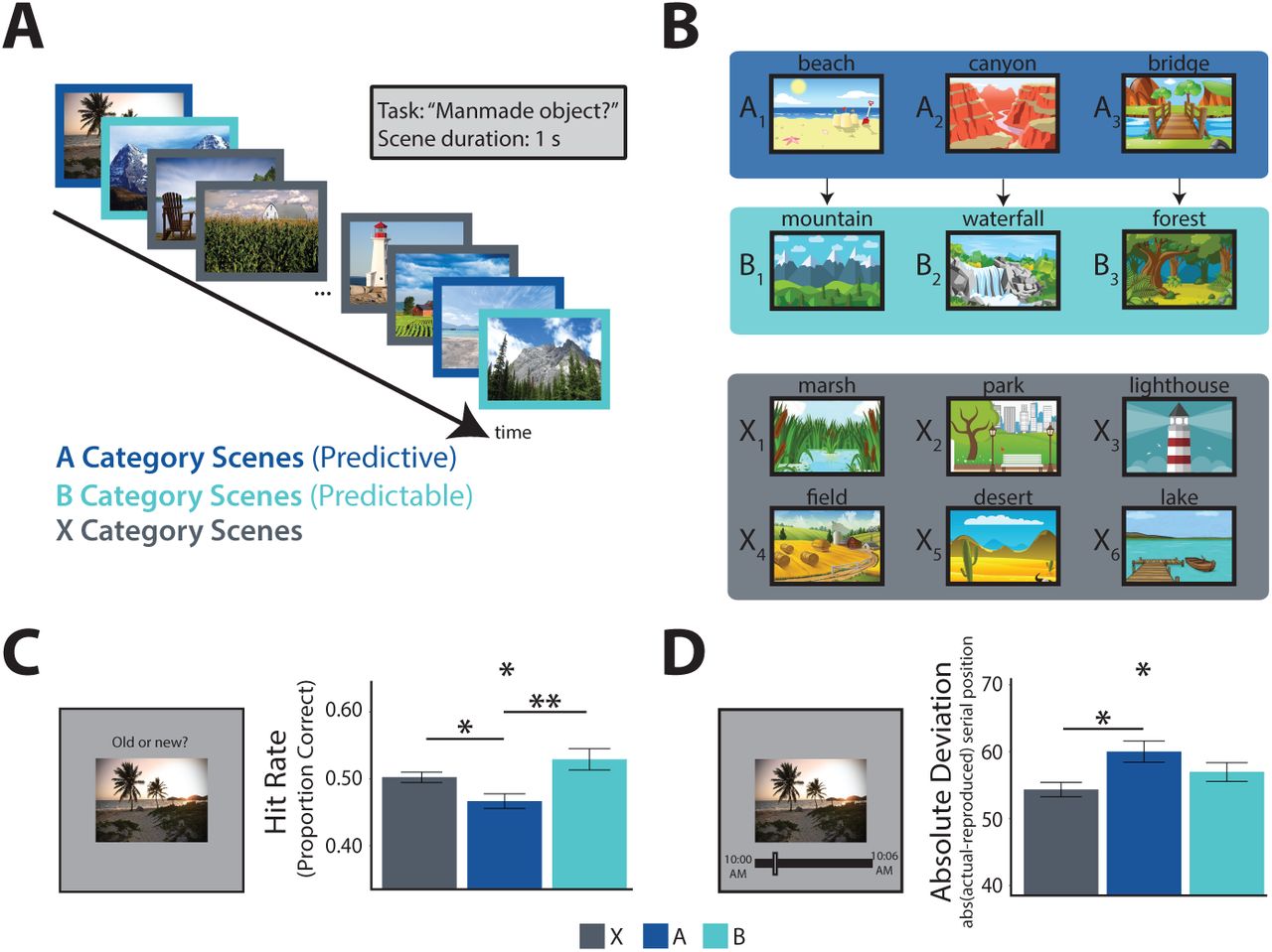
We exposed human participants to a stream of pictures and later tested their memory (Figure 1A). The pictures consisted of outdoor scenes from 12 different categories (e.g., beach, mountain, farm). Three of the categories (type A, predictive) were each reliably followed by one of three other categories (type B, predictable); the remaining six categories (type X, non-predictive, non-predictable) were randomly inserted into the stream. That is, every time participants saw a picture from an A category, they always saw a picture from a specific B category next; however, when a picture from an X category appeared, it was variably preceded and followed by pictures from several other categories (Figure 1B). Participants were not informed about these predictive A → B category relationships and learned them incidentally through exposure (Brady and Oliva, 2008). Although each category was shown several times, every individual picture in the stream was a novel exemplar from the category and shown only once. For example, whenever a picture from the beach category appeared, it was a new beach that they had not seen before. After the stream, we tested memory for these individual pictures amongst new exemplars from the same categories. The key hypothesis was that exemplars from predictive categories would be remembered worse than exemplars from non-predictive categories (Experiments 1 and 2), and that this deficit would be related to predictive processes in the hippocampus (Experiment 3).

Behavioral Experiments. A) Task design: participants viewed a continuous stream of scene pictures, during which they made a judgment of whether or not there was a manmade object in the scene. B) Example scene category pairings for one participant: 3 of 12 categories were assigned to condition A; each was reliably followed by one of 3 different categories assigned to condition B (illustrated by arrows). The remaining 6 categories were assigned to condition X and were not consistently preceded or followed by any particular category. C) Left: surprise recognition memory test. Right: proportion of old exemplars recognized as a function of condition (higher hit rate is better memory). D) Left: temporal source memory test. Right: absolute difference between reported and actual time of encoding as a function of condition (higher deviation is worse memory). Error bars reflect within-participant standard error of the mean. *p <0.05, **p <0.01.
Results
Experiment 1
Encoding Phase
While viewing the stream, 30 participants performed a cover task in which they judged whether or not there was a manmade object in the scene. Participants performed quite well on this task (mean accuracy = 0.91). This performance level was reliably above chance (0.5; t(29) = 42.38, p <0.001). Assessing response times over the course of the experiment, we found a significant main effect of experiment quartile (F(3,87) = 8.30, p <0.001), a marginal main effect of condition (F(2,58) = 3.09, p = 0.053), and an interaction between condition and quartile (F(6,174) = 2.15, p = 0.050). This interaction reflected growing facilitation for the predictable B category, with marginally faster response times by the fourth quartile relative to the X (t(29) = 2.02, p = 0.053) and A (t(29) = 1.99, p = 0.056) categories, whose appearance could not be predicted (Hunt and Aslin, 2001; Olson and Chun, 2001).
Test Phase
To evaluate overall episodic memory performance, we calculated A′ for each participant as a non-parametric measure of sensitivity. All participants had memory performance numerically above the chance level of 0.5 (mean A′ = 0.72, t(29) = 20.02, p <0.001; mean hit rate = 0.50; mean false alarm rate = 0.23). We did not find a significant main effect of condition on A′ (F(2,58) = 2.37, p = 0.10). However, A′ takes into account both the hit rate and the false alarm rate. Given our hypothesis of worse encoding for the old exemplars from the predictive A categories, we expected that hit rate would be a more sensitive measure.
Indeed, there was a main effect of condition on hit rate (F(2,58) = 4.75, p = 0.012), with a lower hit rate for pictures from the A categories relative to both B (t(29) = −2.79, p = 0.0092) and X (t(29) = −2.33, p = 0.027) categories (Figure 1C). There was no difference in hit rate between B and X categories (t(29) = 1.19, p = 0.24), showing that the memory deficit is selective to whether a category was predictive (A vs. X), not whether it was predictable (B vs. X). As hypothesized, this memory deficit reflected a failure to encode specific A exemplars rather than a generic impairment for A categories (De Brigard et al., 2017; Smith et al., 2013), as the false alarm rate for new exemplars from each category at test did not differ by condition (F(2, 58) = 0.29, p = 0.75). Given these findings, analyses in subsequent experiments consider hit rate and false alarm rate separately by condition.
This experiment demonstrated that episodic encoding is worse for predictive vs. non-predictive pictures using a surprise recognition memory test. We interpret this result as evidence of competition between prediction and encoding in the hippocampus. However, recognition tests do not definitively probe aspects of episodic memory that critically depend on the hippocampus. Participants could have relied upon a generic sense of familiarity with the pictures, which can be supported by cortical areas (Brown and Aggleton, 2001; Davachi et al., 2003; Norman and O’Reilly, 2003).
We thus designed Experiment 2 with a different, recall-based memory test. After encoding the same kind of picture stream, participants were unexpectedly asked at test to indicate at what exact time (on the clock) they had seen each picture in the stream. As before, encoding of the time was incidental as they were not informed in advance that they would be tested. This kind of precise temporal source memory requires the retrieval of details about the context in which each picture was encoded, a hallmark function of episodic memory (e.g., remembering who arrived first at a birthday party) that critically depends upon the hippocampus (Davachi and DuBrow, 2015; Miller et al., 2013; Mitchell and Johnson, 2009).
Experiment 2
Encoding Phase
A group of 30 new participants performed quite well on the same manmade cover task as Experiment 1 (mean accuracy = 0.93; relative to 0.5 chance: t(29) = 44.07, p <0.001). There was again a main effect of experiment quartile on response times (F(3,87) = 7.82, p <0.001), but now no main effect of condition (F(2,58) = 0.22, p = 0.80) nor an interaction between condition and quartile (F(6,174) = 0.69, p = 0.65). Despite the lack of a reliable interaction, the overall pattern of results was similar to Experiment 1, with response times in the fourth quartile numerically (though non-significantly) faster for B categories than A (t(29) = 1.03, p = 0.31) and X (t(29) = 1.61, p = 0.12) categories.
Test Phase
In the memory test, participants were presented with a picture and first asked to indicate whether they thought it was old or new, i.e., whether it was presented during the encoding stream. If they indicated that the picture was old, they were then asked to recall when during the stream they had seen the picture. We included the initial old/new recognition judgment because we felt that it would be awkward to ask participants to report the time of a picture they did not remember seeing previously. Nevertheless, our primary hypothesis was that precision of temporal source memory recall would be lower for exemplars from predictive categories, resulting in greater deviation or error for A compared to X categories.
In terms of overall recognition memory from the initial old/new judgments, all participants had an A′ numerically above the chance level of 0.5 (mean A′ = 0.75, t(29) = 23.31, p <0.001; mean hit rate = 0.38; mean false alarm rate = 0.11). Neither the hit rate (F(2,58) = 0.74, p = 0.48) nor the false alarm rate (F(2,58) = 0.33, p = 0.72) differed by condition. The lack of a hit rate effect differed from Experiment 1, but we suspect that this may be an artifact of introducing the source memory task. Specifically, participants in Experiment 2 knew that responding “old” would prompt a difficult follow-up question about their temporal source memory. As a result, they may have strategically adopted a more conservative criterion to avoid the source judgment unless they had a strong memory with high confidence. Consistent with this interpretation, participants were less likely to respond “old” in general in Experiment 2 (mean proportion “old” responses = 0.33) than in Experiment 1 (0.45; t(58) = 4.76, p <0.001).
Regardless, our focus in this experiment was on temporal source memory recall. We assessed overall source memory by computing the average absolute deviation from the correct clock time for all hits. Higher absolute deviation indicates lower precision in memory. The mean absolute deviation across participants was 56.3 pictures, or 84.5 seconds. Using a permutation test, we determined that every participant performed numerically better than chance, indicated by mean deviation less than 69.1 pictures. As hypothesized, there was a main effect of condition on absolute deviation (Figure 1D; F(2,58) = 3.17, p = 0.049). Pictures from the A categories had greater deviation (less precision) than those from the X categories (t(29) = 2.26, p = 0.031), which differed only in that they were not predictive of the upcoming category. Precision as also lower for A relative to B categories, but this difference did not reach significance (t(29) = 1.45, p = 0.16); B and X categories also did not reliably differ from each other (t(29) = 1.23, p = 0.23).
What explains the worse encoding of predictive pictures in Experiments 1 and 2? We propose that this results from the co-dependence of statistical learning and episodic memory on the hippocampus (Schapiro et al., 2017). Specifically, we hypothesize that the appearance of a picture from an A category triggers the retrieval and predictive representation of the corresponding B category in the hippocampus. This in turn prevents the hippocampus from encoding a new representation of the specific details of that particular A picture, which would be needed for later recall from episodic memory. To evaluate this hypothesis, Experiment 3 employed high-resolution fMRI during the encoding phase to link hippocampal prediction to subsequent memory.
Experiment 3 (fMRI)
Encoding Phase Behavior
A group of 36 new participants performed the same manmade cover task as Experiments 1 and 2. Performance across all runs (including the templating phase; see Materials and Methods) remained quite high (mean accuracy = 0.94; relative to 0.5 chance: t(35) = 18.75, p <0.001). Response times were examined across thirds of the encoding phase rather than quartiles because there were three fMRI runs in this phase. We again found a pattern of growing facilitation for the B categories. Although there were no main effects of experiment third (F(2,68) = 0.44, p = 0.65) or condition (F(2,68) = 1.24, p = 0.29), nor an interaction (F(4,136) = 1.17, p = 0.33), response times in the third run were significantly faster for B categories relative to X categories (t(34) = 2.23, p = 0.033); the difference for B relative to A categories was in the same direction but not significant (t(34) = 1.39, p = 0.17).
Test Phase Behavior
In Experiment 3, we returned to the recognition memory task from Experiment 1. All participants exhibited A′ above the chance level of 0.5 except for one, who was excluded from all other behavioral and fMRI analyses (all participants: mean A′ = 0.68, t(36) = 14.63, p <0.001; mean hit rate = 0.61; mean false alarm rate = 0.39). Neither hit rate (F(2,70) = 2.23, p = 0.12) nor false alarm rate (F(2,70) = 0.83, p = 0.44) differed by condition. Although we did not replicate an overall deficit in recognition of A pictures in this experiment, we will leverage variance in condition differences across participants to examine the relationship between memory behavior and neural measures.
Neural Decoding of Perceived Information
The primary purpose of the fMRI experiment was to measure neural prediction during statistical learning in the encoding phase. We used a multivariate pattern classification approach (Cohen et al., 2017), which quantified neural prediction of B categories during the encoding of A pictures. Classification models were trained for each category based on patterns of fMRI activity in a separate phase of the experiment (“pre” templating phase; see Materials and Methods), during which participants were shown pictures from all categories in a random order. These classifiers were then tested during viewing of the encoding stream containing category pairs, providing a continuous readout of neural evidence for each category. We performed this analysis based on fMRI activity patterns from the hippocampus, our primary region of the interest (ROI), as well as from control ROIs in occipital and parahippocampal cortices. These control ROIs were chosen because as visual areas we expected them to be sensitive to the category of the current picture being viewed but not necessarily to predict the upcoming B category given an A picture.
To validate this approach, we first trained and tested classifiers on the viewing of pictures from the A (“Perception of A”) and B (“Perception of B”) categories (Figure 2). Both types of perceptual categories could be decoded in occipital (A: t(35) = 4.34, p <0.001; B: t(35) = 5.96, p <0.001) and parahippocampal (A: t(35) = 3.83, p <0.001; B: t(35) = 3.52, p = 0.0012) ROIs. Interestingly, the perception of B (t(35) = 2.26, p = 0.030) but not A (t(35) = −0.17, p = 0.87) categories could be decoded in the hippocampus.

Category Decoding in fMRI Experiment. Top: Classification accuracy in occipital cortex (OCC), parahippocampal cortex (PHC), and hippocampus (HIPP) for each of the four combinations of training or testing on A or B categories. For every A/B combination and ROI, each dot is one participant and the black line is the mean across participants. Bottom: Regions of interest. HIPP and PHC were manually segmented in native participant space (transformed into standard space for visualization); OCC was defined in standard space and transformed into native participant space.
Neural Decoding of Predicted Information
We next tested the hypothesis that the hippocampus predicts B categories during viewing of the associated A categories. We trained classifiers on pictures from each B category and tested on pictures from the corresponding A category (“Prediction of B”). Crucially, the upcoming B category could be decoded during A in the hippocampus (t(35) = 2.73, p = 0.0098), but this was not possible in occipital (t(35) = 0.94, p = 0.35) or parahippocampal (t(35) = 0.17, p = 0.87) ROIs. Control analyses ruled out potential confounds related to the timing of the fMRI signal: training classifiers on A and testing on B categories (“Lingering of A”), did not yield reliable decoding in the hippocampus (t(35) = 0.96, p = 0.34), nor occipital (t(35) = −0.38, p = 0.71) or parahippocampal (t(35) = 1.57, p = 0.13) ROIs.
Combining these results, there was a trade-off in the hippocampus between category evidence for A and B during the viewing of A, with reliable prediction of B (train on B, test on A) but not perception of A (train on A, test on A). This trade-off was apparent at the individual level: participants with above-chance classification for the upcoming B category (vs. other B categories) had lower classification accuracy for the current A category (vs. other A categories) (t(34) = 2.23, p = 0.033). This suggests that prediction can interfere with the ability of the hippocampus to represent the current item.
The analyses above compared the average classification accuracy across participants against an assumed binary chance level of 0.5. Chance classification can deviate from hypothetical levels for a variety of reasons, so we also performed a non-parametric analysis in which we compared classification accuracy against an empirical null distribution estimated for each participant (see Materials and Methods). This analysis yielded nearly identical results (Figure S1).
To further assess the specificity of these results to the hippocampus, we ran an exploratory whole-brain searchlight analysis. We again validated our approach by decoding the perception of B categories (train on B, test on B). The resulting regions, which represented scene categories, were largely consistent with our a priori control ROIs (Figure S2A). Notably, the prediction of B (train on B, test on A) produced no significant clusters across the brain after correcting for multiple comparisons (Figure S2B), consistent with this effect being specific to the hippocampus ROI.
Relation Between Neural Prediction and Memory Behavior
Finally, we tested our key hypothesis that prediction from statistical learning in the hippocampus is related to impaired encoding of predictive items into episodic memory. We quantified this brain-behavior relationship by correlating (i) each participant’s decoding accuracy for prediction of B during A in the hippocampus with (ii) their difference in hit rate for A vs. X categories in the memory test, which quantifies the relative deficit in memory for predictive items (Figure 3). Consistent with our hypothesis, classification accuracy was negatively correlated with this memory difference (r = −0.33, bootstrap p = .047, two-tailed). That is, greater neural evidence for prediction of the upcoming category was associated with worse encoding of the current exemplar.

Brain-Behavior Relationship in fMRI Experiment. Pearson correlation between “Prediction of B” classification accuracy in the hippocampus during the encoding phase and the difference in hit rate between A and X. The negative relationship indicates that greater hippocampal prediction from statistical learning was associated with worse episodic memory for the predictive item (see also Figure S3). Error shading indicates bootstrapped 95% confidence intervals.
We included all participants in the correlation above, based on the fact that we observed reliable hippocampal prediction of B at the group level. However, some individuals had decoding accuracy at or below chance, which we do not interpret as meaningful variance. To ensure that these individuals were not driving the negative correlation, we re-ran the analysis limited to participants with above-chance prediction of B. If anything, the correlation got stronger (Figure S3; r = −0.63; bootstrap p <0.001, two-tailed).
Discussion
Our findings contribute to growing evidence that the hippocampus plays an important role in statistical learning (Schapiro et al., 2017; Davachi and DuBrow, 2015), including the component processes of prediction (Hindy et al., 2016; Kok and Turk-Browne, 2018) and generalization (Schlichting et al., 2017). In linking these functions to episodic memory, we extend beyond prior work and integrate statistical learning with a broader literature on the role of the hippocampus in memory encoding and retrieval. Specifically, our findings resonate with the observation that encoding and retrieval have fundamentally different requirements (Norman and O’Reilly, 2003; Hunsaker and Kesner, 2013; Neunuebel and Knierim, 2014). Given a partial match between the current experience and past experiences, encoding leverages pattern separation based on the unique features of the current experience and stores a new trace, but in doing so limits access to related old traces. In contrast, retrieval invokes pattern completion to fill out missing features from past experiences and access old traces, but in doing so impedes the storage of a distinct, new trace. To resolve this incompatibility, the hippocampus may toggle between encoding and retrieval states on the timescale of milliseconds to seconds (Hasselmo et al., 2002; Duncan et al., 2012). In the present study, if seeing a picture from an A category triggers pattern completion and activation of its associated B category, the hippocampus may be pushed into a retrieval state that suppresses concurrent memory encoding.
How is this interaction between prediction and encoding implemented in the circuitry of the hippocampus? A recent biologically plausible neural network model of the hippocampus (Schapiro et al., 2017) suggests that episodic memory and statistical learning depend on different pathways, the trisynaptic pathway (TSP) and monosynaptic pathway (MSP), respectively. The TSP consists of connections between entorhinal cortex (EC), dentate gyrus (DG), the CA3 subfield, and the CA1 subfield. In this pathway, DG and CA3 have sparse activity because of high lateral inhibition, which allows them to form distinct representations of similar experiences (i.e., pattern separation) and avoid interference between episodic memories. The MSP consists of a direct connection between EC and CA1. In this pathway, CA1 has lower inhibition and thus higher overall activity and less sparsity, which leads to overlap in the representations of similar experiences, emphasizing their common elements or regularities. Notably, both the TSP and MSP converge on CA1, which is one potential locus of conflict between episodic memory and statistical learning. As an initial exploration of this possibility, we conducted an exploratory functional connectivity analysis (see Supplementary Information). Although our rapid event-related task was not designed for this purpose, we did find some tentative evidence that competition between MSP and TSP connections to CA1 may mediate the tradeoff between episodic memory and statistical learning (Figure S4). Specifically, participants with relatively greater MSP activity (as measured by connectivity between EC and CA1) — the pathway necessary for statistical learning in the computational model referenced above (Schapiro et al., 2017) — exhibited worse episodic memory. Future studies tailored for connectivity analysis and/or employing time-resolved methods such as intracranial EEG are needed to better understand how the hippocampal circuit arbitrates between these two forms of learning.
Our work also raises future questions about the nature of the competition between prediction and encoding. After learning predictive relationships in classical conditioning, “blocking” can occur when new cues are introduced. After one conditioned stimulus (CS1) has been paired with an unconditioned stimulus (US), no associative learning occurs when a second conditioned stimulus (CS2) is added (Kamin, 1969). This is interpreted as CS2 being redundant with CS1, that is, not providing additional predictive value given that the US can be fully explained by CS1. In the present study, the A pictures contain two kinds of features: those that are diagnostic of the category (e.g., sand and water for a beach) and those that are idiosyncratic to each exemplar (e.g., particular people, umbrellas, boats, etc.). If categorical features are sufficient to predict the upcoming B category, idiosyncratic features may not be attended or represented (Mackintosh, 1975; Kruschke, 2001), impeding the formation of episodic memories. Our findings are not fully consistent with this account, however. Blocking might predict that the A pictures are represented more categorically, as this is what enables prediction of the B category. Yet, during the presentation of A pictures we found a trade-off in the hippocampus between neural evidence for perception of the A category and prediction of the B category. Nevertheless, more work is needed to better characterize the deficit in memory for predictive items. Are certain aspects of these memories lost while others are retained? Or are these experiences encoded with less precision overall and/or subject to heightened interference at retrieval? Characterizing associative memory between specific A and B exemplars might be a fruitful avenue for future investigation.
Stepping back, why are the computationally opposing functions of episodic memory and statistical learning housed together in the hippocampus? We propose that this shared reliance might allow them to regulate each other. By analogy, using your right foot to operate both the brake and gas pedals in a car serves as an anatomical constraint that forces you to either accelerate or decelerate, but not both at the same time. A similarly adaptive constraint may be present in the hippocampus, reflecting mutual inhibition between episodic memory and statistical learning. When predictive information is available in the environment, further encoding may be redundant with existing knowledge. Moreover, encoding such experiences could risk over-fitting or improperly updating known, predictive regularities with idiosyncratic or noisy details. By focusing on upcoming events, the hippocampus can better compare expectations and inputs (Kumaran and Maguire, 2006), prioritizing the encoding of novel and unexpected events (Greve et al., 2017; Henson and Gagnepain, 2010).
Author Contributions
Conceptualization, B.E.S. and N.B.T-B.; Methodology, B.E.S. and N.B.T-B.; Investigation, B.E.S.; Formal Analysis, B.E.S.; Writing, B.E.S. and N.B.T-B.; Supervision, N.B.T-B.; Funding Acquisition, B.E.S. and N.B.T-B.
Declaration of Interests
The authors declare no competing interests.
Materials & Methods
Experiment 1
Participants
Thirty individuals (19 female; age range: 18-31, mean age = 21.2) were recruited from the Yale University community for either course credit or $10 compensation. Informed consent was obtained in a manner approved by the Yale University Human Subjects Committee.
Stimuli and Apparatus
Participants were seated approximately 50cm away from a 69cm monitor (1920 × 1080 pixel resolution; 60 Hz refresh rate). Scene stimuli consisted of 300 unique scene images drawn from 12 scene categories (25 images/category), collected from Google image searches. Each participant viewed 22 scenes from each category, randomly selected from the set of 25. Sixteen of these images (per each category; 192 total) were used in the encoding phase, two for the category pair test, and four as foils in the recognition test. Scene stimuli were presented centrally and subtended 27.8 × 20.8 degrees of visual angle. Stimuli were presented using MATLAB (The MathWorks, Natick, MA) with the Psychophysics Toolbox (Brainard and Vision, 1997; Pelli and Vision, 1997).
Procedure
Participants first completed an encoding phase. On each trial, they viewed a photograph of a scene for 1000 ms, during which they had to respond based on whether it contained a manmade object (Figure 1A). Participants were instructed to respond as quickly and accurately as possible (response mappings of ‘j’/’k’ onto ‘yes’/’no’ were counterbalanced across participants), and we recorded response time and accuracy. The scene remained on the screen for 1000 ms regardless of button press to equate encoding time, and trials were separated by a 500-ms inter-stimulus interval (ISI) during which a fixation cross appeared.
Every scene was trial-unique, but was drawn from one of 12 outdoor scene categories (beaches, bridges, canyons, deserts, fields, forests, lakes, lighthouses, marshes, mountains, parks, and waterfalls; Figure 1B). Each scene category appeared 16 times over the course of the encoding phase, for a total of 192 trials. The photographs for half of the scene categories always contained a manmade object, and thus all exemplars in a category required the same response, and the responses were balanced overall. Unbeknownst to participants, and orthogonal to the required response, half of the scene categories were assigned to pairs. Given the first scene in a pair (A category scenes), the category of the second scene (B category scenes) was predictable with a transition probability of 1.0. The other half of scene categories were neither predictive nor predictable (X category scenes). Pictures from these categories were inserted on their own randomly, with the constraint that they could not be placed between an A category scene and a B category scene. The assignment of scene categories to A/B/X conditions was itself randomized for each participant. The order of the photograph sequence was randomized with the following three constraints: category pairs and pairs of category pairs could not repeat back-to-back (i.e., no A1B1A1B1 or A1B1A2B2A1B1A2B2, where 1 and 2 index different exemplars); repetitions of each category were spread equally across quartiles of the encoding phase to minimize differences in study-test lag between categories; and the overall transition probability between “yes” and “no” responses on the manmade cover task was forced to be statistically indistinguishable from 0.5.
After the encoding phase, participants performed five minutes of a distracting math phase to minimize recency effects. Each of 60 math problems consisted of division and subtraction, and the answer to the problem was always 1, 2, 3, or 4. Participants responded using the 1, 2, 3, and 4 keys on the keyboard, with a maximum response window of 5 s. The ISI was adjusted based on the response time (5 s minus response time), to ensure that this phase lasted exactly 5 min given the 60 trials. Participants were instructed to respond as accurately as possible.
Participants then underwent two surprise memory tests (category pair test and episodic memory test), the order of which was counterbalanced across participants. The category pair test involved explicit judgments of the category pairings from the encoding phase. Participants were presented with two pairs of photographs on every test trial and were asked to indicate which pair felt more familiar based only what they had seen during the encoding phase. The pairs were shown sequentially: the first scene from one pair appeared for 1000 ms, followed by a 500-ms blank interval, followed by the second scene of the pair for 1000 ms; after a 1000 ms gap with a fixation cross, a second pair was presented in the same manner. After both pairs, participants responded using the ‘1’ key to indicate if the first pair felt more familiar or the ‘2’ key if the second pair felt more familiar. Participants had a maximum of 6 s to respond. Each scene in the category pair test was a completely novel exemplar of its category. Half of the test trials contained a true category pair (when it was a trial testing a pair from the encoding phase); whether it appeared first or second was counterbalanced. The other half of the trials contained a “dummy coded” pair of the X categories (there was no correct answer on these trials). This was done to equate the frequency of categories, which was important for participants who received the category pair test before the episodic memory test. Each true/dummy-coded pair was tested twice against a scrambled pair of the same categories (e.g., if beach → field, mountain → bridge, canyon → forest were category pairs from the encoding phase, the foils might be beach → bridge, mountain → forest, canyon → field). Performance on this category pair test for true pairs vs. scrambled pairs was not reliable in either Experiment 1 (mean accuracy = 0.48; vs. 0.5 chance: t(29) = −0.72, p = 0.48) or Experiment 2 (mean accuracy = 0.49; vs. 0.5 chance: t(29) = −0.61, p = 0.55), nor did the order of the category pair test and episodic memory test affect episodic memory behavior. Thus, the results of the category pair test are not reported further and this test was not included in Experiment 3.
The episodic memory test was designed to assess episodic memory for the trial-unique scenes from the encoding phase. On each trial, one scene was presented and participants indicated whether it was “old” (i.e., presented during the encoding phase) or “new” (i.e., not previously seen in the experiment). After making an old/new response (using ‘j’/’k’ keys on the keyboard), participants then rated their confidence in this response (“not confident”/”confident”, using ‘d’/’f’ keys). Participants had 6 s to make each response. All 192 scene photographs from the encoding phase were shown, in addition to 48 foils (4 novel exemplars from each category). The order of the scenes was randomized.
Experiment 2
Participants
Thirty individuals (19 female; age range: 18-23, mean age = 19.3) were recruited from the Yale University community for either course credit or $10 compensation. Informed consent was obtained in a manner approved by the Yale University Human Subjects Committee.
Stimuli and Apparatus
Same as Experiment 1.
Procedure
The procedure was identical to that of Experiment 1, with the addition of a temporal source memory judgment in the test phase. That is, participants were presented with a scene and first asked to judge whether it was “old” or “new” (using the ‘d’ and ‘f’ keys). Then, old responses were followed by the presentation of a timeline, bound by the start and end clock times of the encoding phase. Participants used the mouse to click along the timeline to indicate when they remembered seeing the scene. No temporal source judgments were collected after new responses.
Experiment 3
Participants
Thirty-eight individuals (24 female; age range: 18-35, mean age = 23.1) were recruited from the Yale University community for $30 compensation. Informed consent was obtained in a manner approved by the Yale University Human Investigation Committee. One participant was excluded to due a neurological anomaly, and one participant was excluded for chance-level episodic memory performance (overall A′ <0.5). Additionally, one participant was excluded from response time analyses because of a technical error that resulted in no responses being collected for part of the encoding phase.
Stimuli and Apparatus
Stimuli were presented on a rear-projection screen using a projector (1920 × 1068 pixel resolution; 60 Hz refresh rate). Participants viewed the stimuli through a mirror mounted on the head coil. Scene stimuli consisted of 480 unique images drawn from 12 categories (40 images/category), collected from Google image searches (180 additional stimuli were collected for this experiment; the other 300 are identical to those used in Experiments 1 & 2). Each participant viewed 39 scenes from every category, randomly selected from the set of 40: 21 per category (252 total) for the encoding phase, 14 (168) for the pre and post templating phases, and 4 (48) as foils in the episodic memory test.
Procedure
The procedure was identical to Experiment 1 other than the following changes:
Instead of one continuous block of the encoding phase (with 16 repetitions of each scene category), the stream was divided into three fMRI runs, each with seven repetitions/category (such that were 21 repetitions/category in total across the encoding phase). As in Experiments 1 & 2, each image was presented for 1 s, but the ISI varied between 2 s (39.3% of trials), 3.5 s (39.3% of trials), and 5 s (21.4% of trials) to jitter onsets for deconvolving event-related fMRI activity. For the manmade object cover task, participants responded using their right index and middle fingers on an MR-compatible button box.
Before and after the three runs of the encoding phase there were “pre” and “post” templating phases (one fMRI run each). To participants, these phases were identical to the encoding phase (e.g., stimulus timing and task were identical). However, there were no category-level regularities in these two runs. Scenes from all categories were presented in a random order. To limit the impact of this random presentation on subsequent learning, participants completed a distracting math task between the “pre” templating run and the first encoding phase run. Each of these five functional runs (three encoding phase runs and pre/post runs) lasted 6.4 minutes.
For the episodic memory test, as in Experiment 1, a scene was presented and participants indicated (with their index and pinky fingers) whether it was “old” (i.e., presented during the encoding phase) or “new” (i.e., not previously seen in the experiment). They then rated their confidence in this response (“very unsure”,”unsure”,”sure”,”very sure”), using their index through pinky fingers, respectively. Participants had 6 s to respond to each of these questions. They completed this task while in the scanner, but no fMRI data were collected. No category pair test was administered in this experiment.
MRI Acquisition
Data were acquired on a Siemens Prisma 3T scanner using a 64-channel head coil at the Magnetic Resonance Research Center at Yale University. Functional images were acquired using an EPI sequence with the following parameters: TR = 1500 ms; TE = 32 ms; 90 axial slices; voxel size = 1.5 × 1.5 × 1.5 mm; flip angle = 64 degrees; multiband factor = 6. Additionally, a pair of opposite phase-encode spin-echo volumes were collected for distortion correction (TR = 11,220 ms; TE = 66 ms). One T1-weighted MPRAGE (TR = 1800 ms; TE = 2.26 ms; voxel size = 1 × 1 × 1 mm; 208 sagittal slices; flip angle = 8 degrees) and two T2-weighted turbo spin echo (TR = 11,390 ms; TE = 90 ms; 54 coronal slices; voxel size = 0.44 × 0.44 × 1.5 mm; distance factor = 20%; flip angle = 150 degrees) anatomical images were collected.
fMRI Preprocessing
fMRI data processing was carried out using FEAT (fMRI Expert Analysis Tool) Version 6.00, part of FSL (FMRIB’s Software Library, www.fmrib.ox.ac.uk/fsl) version 5.0.10. EPI and anatomical images were skull-stripped using the Brain Extraction Tool (Smith, 2002). Susceptibility-induced distortions measured via the opposing-phase spin echo volumes were corrected using FSL’s topup tool (Andersson et al., 2003). Each functional run was high-pass filtered with a 128 s period cut-off, corrected for head motion using MCFLIRT (Jenkinson et al., 2002), and motion outliers were computed. Slice-timing correction was performed. No spatial smoothing was applied. Lastly, the six motion parameters, as well as motion outliers, were regressed against the BOLD timecourse using a general linear model (GLM). The residuals from this preprocessing model (which contain BOLD responses to the task after controlling for motion) were then used for subsequent analyses.
Functional images were registered to each participant’s T1 anatomical scan using boundary-based registration, as well as to a 2 mm MNI standard brain, using 12 degrees of freedom. Lastly, the two T2 anatomical images collected were registered to one another and averaged; the resulting averaged image was registered to the T1 anatomical image using FLIRT (Jenkinson and Smith, 2001).
Regions of Interest
Our primary region of interest (ROI) was the hippocampus. Hippocampal subfields CA1, CA2/3/DG, and subiculum, as well as medial temporal lobe (MTL) cortical regions entorhinal cortex (EC), perirhinal cortex (PRC), and parahippocampal cortex (PHC) were manually segmented on participants’ averaged T2 anatomical scan (Figure S4A), using published criteria on anatomical landmarks (Insausti et al., 1998; Pruessner et al., 2002; Duvernoy, 2005; Aly and Turk-Browne, 2015). Corresponding ROIs from each hemisphere were concatenated to create one bilateral ROI per region, as we had no hemisphere-specific hypotheses. A bilateral whole hippocampus ROI was created by concatenating the three bilateral subfield ROIs. Individual ROIs were transformed into each participant’s functional space for subsequent analyses. The occipital cortex ROI was defined using the MNI structural atlas, thresholded at 25% probability. This standard space ROI was then transformed into each participant’s functional space for subsequent analyses.
Category Decoding Analysis
A multivariate pattern classification approach was used to assess evidence for a particular category during the encoding phase. This approach involved training a classifier on fMRI activity patterns for each category from the “pre” templating run (when there were no regularities present and none had been learned) and testing for classifier evidence of these categories during the three (independent) runs of the encoding phase.
For each functional run, the residuals from the preprocessing GLM (with known noise sources removed but still containing task responses) were aligned to the final functional run and z-scored across time. The voxel x time matrices were then masked to only include voxels within an ROI. The timepoints corresponding to the presentation of each of two categories of interest were extracted and shifted by 3 TRs (4.5 seconds) to account for the hemodynamic lag. The voxel activity patterns from these shifted time points were then used as training or test data for the classifier. Timepoints that included a motion outlier were excluded from the training/test sets.
Linear SVMs were trained on data and labels from the pre-learning templating run, using the SVC function in Python’s scikit-learn module, with a penalty parameter of 1.00. Classifiers were then tested with data corresponding to the timepoints of the trained categories in the three runs of the encoding phase (concatenated) and made guesses as to the category label of each test example. Accuracy was computed as the proportion of correct guesses.
We ran the following comparisons: Perception of A (training on pre-learning examples of A, testing for evidence of A during the presentation of A in the encoding phase), Perception of B (training on pre-learning examples of B, testing for evidence of B during the presentation of B in the encoding phase), Lingering of A (training on pre-learning examples of A, testing for evidence of A during the presentation of B in the encoding phase), and Prediction of B (training on pre-learning examples of B, testing for evidence of B during the presentation of A in the encoding phase).
Each participant encountered three A and three B categories over the course of the experiment. Thus, for each of the four comparisons above, we built three different binary classifiers and then averaged their accuracy. In other words, a classifier was trained to distinguish between two scene categories from the same condition (e.g., B) based on the pre-learning templating run, and tested for evidence of those two categories during the subsequent presentation of two categories (e.g., their corresponding As for Prediction of B) in the encoding phase. Accuracy (percent correct) was then computed for each of these three classifiers (A1 vs. A2; A2 vs. A3; A1 vs. A3) and averaged, resulting in one mean accuracy value per comparison, per participant.
To provide an example, if the category pairs were beach → field, mountain → bridge, canyon → forest, then B classifiers would be trained for field vs. bridge, bridge vs. forest, and field vs. forest. To calculate evidence for Prediction of B: the field vs. bridge classifier would be applied to the beach and mountain trials — such that the classifier estimated evidence for field and bridge during each beach or mountain trial — and accuracy was computed (such that, for example, accuracy on a beach trial was 1 if the classifier outputted more evidence for field than for bridge). This was repeated for the bridge vs. forest classifier (testing for evidence of these categories during mountains and canyons) and the field vs. forest classifier (testing for evidence of these categories during beaches and canyons). The accuracies of these three classifiers were averaged into a single accuracy for each participant. This was repeated for the three other comparisons above and for each ROI. To assess reliability at the group level, performance was compared to a chance level of 0.50 across participants using a one-sample t-test.
To quantify classification accuracy non-parametrically, we performed randomization tests in which we computed an empirical null distribution of classification accuracy values for each participant. The null distributions were generated from 1,000 iterations of shuffling the category labels at test prior to scoring the model. We then calculated a z-score for each participant’s true classification accuracy relative to their own null distribution. To test reliability, we compared these z-scores against 0 across participants (Figure S1).
Assessing Reliability of Correlations
To estimate correlations across participants robustly (e.g., as used in the Relation Between Neural Prediction and Memory Behavior section), we performed a random-effects bootstrap resampling procedure (Efron and Tibshirani, 1986). For each of 10,000 iterations, we randomly drew 36 participants from our sample with replacement, and recalculated the Pearson correlation between the two variables of interest. This procedure operates under the assumption that if the effect is reliable across participants, then the participants are interchangeable and which subset is resampled in any given iteration will not affect the outcome. This approach also helps mitigate the impact of outliers when calculating correlations from modest sample sizes. The resulting sampling distribution can be used to generate confidence intervals and perform null hypothesis testing. Specifically, we calculated the p value as the proportion of iterations in which the correlation value was of the opposite sign from the true correlation, then multiplied by 2 for a two-tailed significance.
Data Availability
fMRI data can be downloaded from OpenNeuro and behavioral data can be downloaded from Dryad.
Acknowledgments
This work was supported by NSF GRFP to B.E.S., as well as NIH R01 MH069456, NSF CCF 1839308, and the Canadian Institute for Advanced Research to N.B.T-B.
References


