

Abstract
Over 15 million epilepsy patients worldwide do not respond to drugs. Successful surgical treatment requires complete removal, or disconnection of the seizure onset zone (SOZ), brain region(s) where seizures originate. Unfortunately, surgical success rates vary between 30%-70% because no clinically validated biological marker of the SOZ exists. We develop and retrospectively validate a new EEG marker - neural fragility. We validate this new marker in a retrospective analysis of 91 patients by using neural fragility of the annotated SOZ as a metric to predict surgical outcomes. Fragility predicts 43/47 surgical failures with an overall prediction accuracy of 76%, compared to the accuracy of clinicians being 48% (successful outcomes). In failed outcomes, we identify fragile regions that were untreated. When compared to 20 EEG features proposed as SOZ markers, fragility outperformed in predictive power and interpretability suggesting neural fragility as an EEG fingerprint of the SOZ.
1 Introduction
Over 15 million epilepsy patients worldwide and 1 million in the US suffer from drug-resistant epilepsy (DRE) [1–5]. DRE is defined as continued seizures despite adequate trials of two tolerated appropriately chosen anti-epileptic drugs [6]. DRE patients have an increased risk of sudden death and are frequently hospitalized, burdened by epilepsy-related disabilities, and the cost of their care is a significant contributor to the $16 billion dollars spent annually in the US treating epilepsy patients [7, 8]. Approximately 50% of DRE patients have focal DRE, where a specific brain region or regions, termed the epileptogenic zone (EZ), is necessary and sufficient for initiating seizures and whose removal (or disconnection) is necessary for complete abolition of seizures [9–12]. The EZ encompasses the clinically identified seizure onset zone (SOZ) and early propagation zone (EPZ). The brain regions associated with the SOZ demonstrate the earliest electrophysiological changes during a seizure event, and in general precede the clinical onset of seizures; and the EPZ regions are involved at the time of the earliest clinical (semiological) manifestations during a seizure event. Successful surgical and neuromodulatory treatments can stop seizures altogether or allow them to be controlled with medications [13–15], but outcomes for both treatments critically depend on accurate localization of the SOZ.
Localizing the SOZ also relies on accurate placement of electrodes such that they cover the EZ, and the ability to identify abnormalities in the iEEG channels that may correlate to the SOZ with the naked eye. Unfortunately, even the most experienced clinicians are challenged because epilepsy is fundamentally a network disease, which cannot be entirely defined by the current methods of localization. Abnormal connections across several channels may constitute a more effective marker of the SOZ [16]. Localization thus lends itself to a data-driven network-based computational approach and several EEG algorithms have been proposed to localize the SOZ from recordings. Many entail investigations of the spectral power in each iEEG channel including high frequency oscillations [17–23], but these approaches do not consider network properties of the brain because they treat each EEG channel independently. Others have proposed graph-based analysis of iEEG [24–35], but these approaches fail to identify internal network properties that cause seizures to occur in the first place.
In this study, we propose a new EEG marker of the SOZ, neural fragility, of brain regions. To create our fragility marker, we first build a personalized dynamic model of the brain network from observed iEEG signals. The model is generative in that it can accurately reconstruct the patient’s iEEG recordings [36, 37]. Using this model, we then calculate which network nodes are imbalanced, meaning they have more excitatory or less inhibitory influence on the network and thus can trigger seizures. Neural fragility measures the degree to which a node is imbalanced [38]. To evaluate neural fragility as a marker of the SOZ, we conducted a retrospective study using iEEG data from 91 patients treated across 5 epilepsy centers: Johns Hopkins Hospital, National Institute of Health, Cleveland Clinic, University of Maryland Medical Center and Jackson Memorial Hospital, University of Miami. In the study population, all DRE patients underwent invasive iEEG monitoring followed by surgical resection or laser ablation of the SOZ (44 success and 47 failure outcome). We demonstrate that neural fragility is higher/lower in electrode contacts within clinically annotated SOZs for success/failure patients. In addition, we compare fragility of iEEG nodes to 6 frequency-based and 14 graph theoretic features in a 10-fold nested-cross validation. Neural fragility has an area under the curve (AUC) discrimination score of 0.88 ± 0.064, which is 13% better compared to the next best feature. In addition, it has a high degree of interpretability, which we demonstrate by computing an interpretability ratio suggesting that the spatiotemporal heatmaps of neural fragility are a robust iEEG fingerprint of the SOZ that can incorporate seamlessly into the clinical workflow.
2 Results
Once the SOZ is localized, the EPZ is often straightforward to identify. In fact, the SOZ forms an important component for the location of the underlying EZ [39–44]. There is no clinically validated biomarker of the SOZ. This presents a serious challenge for clinicians to accurately localize the SOZ and has led to surgical success rates to vary between 30-70% despite large brain regions being removed. With no biomarker available, clinicians are driven to perform extensive evaluations with neuroimaging, clinical testing, and visual inspection of scalp electroencephalography (EEG) recordings. When non-invasive tests are inconclusive, patients undergo intracranial monitoring, during which intracranial EEG (iEEG) electrodes are either placed directly on the cortex or implanted into the brain (example in Supplemental Figure S1). iEEG provides high temporal resolution data that enables clinicians to visually detect abnormal activity, such as spikes and high frequency bursts, in between seizures (interictal) and during seizures (ictal). Specifically, clinicians attempt to identify the electrodes involved in the SOZ and early spread [11, 12, 45–47]. Surgical resection is then performed on the basis of this hypothesis, unless the region overlaps with eloquent cortex [48].
We analyze all patient’s iEEG using fragility and 20 other baseline features, resulting in spatiotemporal heatmaps per patient for every feature. The baseline features include spectral power in various frequency bands (e.g. delta band 1-4 Hz) and specific graph measures of bivariate correlation measures (e.g. eigenvector centrality and degree of correlation and coherence matrices), which have been previously reported in the literature to correlate to the SOZ [25–31, 35, 49]. We consider all of these as potential EEG features that can represent the data in different ways, potentially useful for SOZ localization.
2.1 Description of Neural Fragility
Neural fragility is a paradigm shift in the EEG analytics space. It is a concept based on the conjecture that focal seizures arise from a few fragile nodes, i.e., the SOZ, which renders the cortical epileptic network on the brink of instability. We begin with an intuitive explanation of neural fragility in Figure 1 (for a two-node quantitative example, see Supplemental Figure S3). When one observes iEEG data during interictal, or preictal periods (Figure 1, top left), activity recorded from each channel is noisy and hovers around a baseline value. In contrast, when one observes iEEG data during a seizure event (Figure 1, top right), activity (i) grows in amplitude, (ii) oscillates, and (iii) spreads in the brain. From a dynamical systems perspective, the iEEG network has switched from a stable (non-seizure) to an unstable (seizure) network. The only difference between the left and right iEEG network in Figure 1 is the connection strengths representing the dynamical interactions between a few channels, i.e., the SOZ. Our conjecture is that small changes in connection strengths at SOZ nodes cause an imbalance in connectivity between inhibitory (I) and excitatory (E) populations (nodes) in the region. Either inhibition is decreased and/or excitation is increased; thus, if the SOZ is perturbed then over excitation can occur manifesting in a seizure.

(Top) iEEG traces in between seizures (left) and during a seizure (right). (Bottom) network schematic showing change in connectivity (right) in fragile node that causes seizure. This describes qualitatively the concept of neural fragility in the context of a dynamical iEEG network, with nodes representing excitatory (E) and inhibitory (I) population of neurons. From a dynamical systems point of view, such imbalance arises from a few fragile nodes causing instability of the network in the form of over-excitation, or under-inhibition. We introduce the fragility of a network node in [36, 38] and define it to be the minimum perturbation applied to the node’s functional connectivity to its neighbors before rendering the network unstable. In system theory, stable systems return to a baseline condition when a node is perturbed. In contrast, unstable systems can oscillate and grow when a node is perturbed. In the context of epilepsy, a fragile node is one that requires a smaller perturbation to lead to seizure activity.
2.2 Fragility heatmap highlights the clinical SOZ in successful patients
To qualitatively assess the usefulness of fragility in localizing electrodes of interest, we first look at specific examples of patients analyzed with fragility and demonstrate how it may provide additional information for SOZ localization. In Figure 3, we show an example of three different patients with differing surgical treatments, outcomes, Engel class and clinical complexity along with their fragility heatmaps and corresponding raw iEEG data (for full clinical definitions; see Supplementary Excel table).
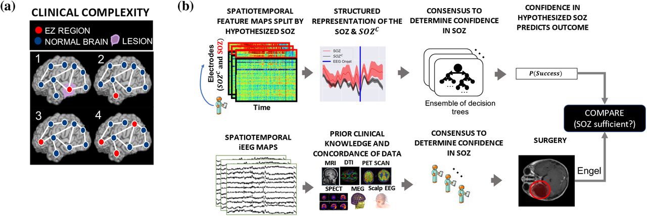
(a) Schematic of the difficulty of different epilepsy etiologies that might arise in DRE patients. Since there is no biomarker for the EZ and it is never observed directly, the network mechanisms that cause seizures are complex. Case clinical complexity ordered by increasing localization difficulty: lesional (1), focal temporal (2), focal extratemporal (3), and multi-focal (4) that are present in the dataset. These four categories simplify the possible EZ presentations, but provide a broad categorization of simple to complex cases observed in the clinic. After non-invasive analysis is inconclusive, a complex and relatively lengthy iEEG workflow for localization takes place (see Supplemental Figure S1 for full details). (b) Is a schematic of our experimental design. (top row) We evaluated various representation of the iEEG data in the form of spatiotemporal heatmaps computed, created a partitioned summary of the SOZ and SOZC around seizure onset based on clinical annotations, fed them into a Random Forest classifier and computed a probability of success (i.e. a confidence score) in the clinically hypothesized SOZ. The probability was then compared with the actual outcome of subjects. (bottom row) Shows an analogous workflow that clinicians take to evaluate their confidence in a proposed SOZ localization resulting in a surgery. During invasive monitoring, clinicians identify the SOZ from iEEG patterns (e.g. HFOs, or spiking/rhythmic activity). An estimate of the true EZ is then created using a combination of the clinical SOZ hypothesis, as well non-invasive findings. When possible, subsequent surgical resection or laser ablation, generally including the SOZ along with a variable extent of additional tissue, is performed. Post-operatively, patients are followed for 12+ months and categorized as either success, or failure as defined in Section 6.1. This translates to clinical outcomes measured by Engel score. In order for a feature to be an accurate representation of the underlying epileptic phenomena, the following assumptions are made. As a result of seizure freedom, one can assume that the clinically hypothesized SOZ was sufficient, and the probability of success has a high value. In contrast, if seizures continue, then the SOZ was not sufficient and the probability should have a low value.

Fragility heatmaps, and corresponding raw EEG traces of successful and failed outcome patients. (a) From top to bottom, Patient_1 (success, treated at NIH, CC1, Engel score 1), Patient_26 (failure, treated at Cleveland Clinic, CC3, Engel score 4), and Patient_40 (failure, treated at Cleveland Clinic, CC4, Engel score 3) are shown respectively. The color scale represents the amplitude of the normalized fragility metric, with closer to 1 denoting fragile regions and closer to 0 denoting relatively stable regions. (Left) Overlaid average neural fragility value of each electrode in the window of analysis we used. Black dark squares represent a depth electrode that is not shown easily on the brain. Black lines outline where the clinicians labeled SOZ. Note in Patient_26, RAD and RHD electrodes are denoted by the squares with the color showing the average over the entire electrode. (Right) Clinically annotated heatmaps of the implanted ECoG/SEEG electrodes with red y-axis denoting SOZ contacts. The red contacts are also part of the surgical resection in these patients. Data is shown in the turbo colormap. Best seen if viewed in color. (b) Corresponding raw EEG data for each patient with electrodes on y-axis and time on x-axis with the dashed white-lines denoting seizure onset. Each shows 10 seconds before seizure onset marked by epileptologists, and 10 seconds after. EEG was set at a monopolar reference with line noise filtered out, according to Section 6.3. Each EEG snapshot is shown at a fixed scale for that specific snapshot that was best for visualization, ranging from 200 uV to 2000 uV.
In Figure 3a, the red electrode labels on the y-axis correspond to the clinical SOZ electrodes; note that the red electrodes are typically a subset of the resected region. This figure shows the period 10 seconds before and after electrographic seizure onset, indicated by the black dashed line. In Patient_1, the clinical SOZ shows a high degree of fragility, even before seizure onset, which is not visibly clear in the raw EEG. The heatmap for Patient_1 also captures the propagation of seizure activity (Supplementary Figure S8). This patient had a successful surgery, and so we can assume the epileptogenic tissue within the clinical resection likely contained the SOZ and EPZ regions; it is likely the clinicians correctly localized the EZ. When viewing the raw EEG data in Figure 3b (top), Patient_1 has iEEG signatures that are readily visible around seizure EEG onset (Figure 3b). We see high-frequency and synchronized spiking activity at onset that occurs in electrodes that clinicians annotated as SOZ, which correspond to the most fragile electrodes at onset. In addition, the fragility heatmap captures the onset in the ATT and AD electrodes and early spread of the seizure into the PD electrodes. Specifically, ATT1 (anterior temporal lobe area) shows high fragility during the entire period before seizure onset (Figure 3). This area was not identified with scalp EEG, or non-invasive neuroimaging. In this patient, the fragility heatmap agreed with clinical visual EEG analysis, identifying the SOZ, which was included in the surgery and led to a seizure free patient.
2.3 Fragility heatmap highlights other possibly epileptic regions outside the SOZ in failed patients
In Figure 3, Patient_26 and Patient_40 both show distinct regions with high fragility that were not in the clinically annotated SOZ (or the resected region), and both had recurrent seizures after surgery. Specifically in Patient_26, the ABT (anterior basal temporal lobe), PBT (posterior basal temporal lobe) and RTG29-39 (mesial temporal lobe) electrodes were highly fragile, but not annotated as SOZ. Patient_40 had laser ablation performed on the electrode region associated with Q2, which was not fragile. From seizure onset, many electrodes exhibit the EEG signatures that are clinically relevant, such as spiking and fast-wave activity [46]. In this patient, the X’ (posterior-cingulate), U’ (posterior-insula) and N’/M’/F’ (superior frontal gyrus) were all fragile compared to the Q2 electrode, which recorded from a lesion in the right periventricular nodule. Patient_26 had a resection performed in the right anterior temporal lobe region. Clinicians identified the RAD, RHD and RTG40/48 electrodes as the SOZ. In the raw EEG data, one can see synchronized spikes and spike-waves in these electrodes, but the patient had seizures continue after resection. In the corresponding fragility heatmap, the ABT and the RTG29-32 electrodes are highly fragile compared to the clinically annotated SOZ region. In the raw EEG shown in Figure 3b, it is not visibly clear that these electrodes would be part of the SOZ. Visual analysis of the EEG was insufficient for Patient_26 and Patient_40, which ultimately led to insufficient localizations and then to failed surgical outcomes. Based on the fragility heatmaps, the fragile regions could be hypothesized to be part of the SOZ, and possibly candidates for resection.
2.4 Fragility outperforms all iEEG features in predicting surgical outcomes
To test the validity of neural fragility and the baseline features as SOZ markers, we investigate each feature’s ability to predict surgical outcomes of patients when stratified by the set of SOZ contacts and the rest which we denote as the SOZ complement, SOZC. To do so, we trained a Structured Random Forest model (RF) [50–52] for each feature that takes in a partitioned spatiotemporal heatmap based on the clinically annotated SOZ and generates a probability of success - a confidence score in the clinical hypothesis. We test each feature’s model on a held out data set by applying a varying threshold to the model’s output and computing a receiver operating characteristic (ROC) curve. The ROC curve plots true positive rates versus false positive rates and the area under the curve (AUC) is a measure of discriminative power of the feature. The larger the AUC, the more predictive the feature is and thus the more valid it is as an iEEG marker of the SOZ. We also compute the precision (PR) or positive predictive value (PPV) for each feature, which is the proportion of predicted successful or “positive” results that are true positives (actual successful surgeries). In addition, we compute the negative predictive value (NPV) as well. The larger the PPV/NPV, the more predictive the feature is and thus the more valid it is as an iEEG marker of the SOZ.
Since each patient’s implantation has a varying number of electrodes, we summarize each feature’s distribution of the SOZ and SOZC electrodes into quantile statistics over time (for details, see Methods 6). As an input to the RF models, we compute the quantile statistics over time of the SOZ and SOZC set for each patient and each feature. This allows each patient’s heatmaps to have the same dimensions, which can be input into a machine learning RF model. RF models are attractive because they are non-parametric, are interpretable (they are just a set of decision trees performing a consensus procedure), and are able to handle higher dimensional data better compared to other models, such as Logistic Regression [53]. As an output of the trained RF model, each heatmap gets mapped to a probability that the outcome will be a success. An RF model is tuned for each feature through 10-fold cross-validation (CV; see Methods section for full details), resulting in a uniform and rigorous benchmark against neural fragility on the same set of subjects. Note that the “high-gamma” frequency band feature encompasses what some would consider HFOs (i.e. 90-300 Hz) activity. In terms of AUC (measures discrimination), neural fragility performs the best (Figure 4a). Compared to the top 3 leading baseline features, neural fragility outperforms the beta band (15-30 Hz) power by more than 13%. The AUC of fragility is the highest with a value of 0.88 ± 0.064, compared to the next best representation, the beta frequency band, with a value of 0.82 ± 0.040. From the ROC (and PR) curves, we observe that the fragility consistently has a higher sensitivity for the same false positive rate compared to the 20 other feature representations (Supplemental Figure S10). In terms of effect size, neural fragility improves over the beta frequency band with a large [54] effect size of 0.97 Cohen’s D with 9 out of 10 folds improving the AUC (Paired Wilcoxon Rank-sum PValue = 0.027 (see Supplemental Figure S10). As a result of the 10-fold CV, we can compare the AUC on the same set of subjects in a paired effect size and statistical test improving AUC on 9 out of the 10 CV folds.

Specific results for neural fragility are marked in red for each of the panels (a-d). (a) Discrimination plot (measured with AUC) shows the relative performance of benchmark feature representations compared to that achieved with neural fragility. (b) A similar average-PR curve shows the relative positive predictive value of all features compared with fragility. Average precision is the analagous area under the curve for the PR curve. (c) A summary of the Cohen’s D effect size measurements between the success and failed outcome CS distributions across all features. The effect size of neural fragility is significantly greater then that of the beta band (alpha = 0.05) (d) The corresponding PValues of the effect size differences between success and failed outcomes, computed via the Mann-Whitney U-test.
In terms of PR (measures PPV), neural fragility also performs the best (Figure 4b). IN terms of average precision, which weighs the predictive power in terms of the total number of subjects, neural fragility also obtains an average precision of 0.83 ± 0.076, which is >5% better than the next best feature. In addition, compared to the clinical surgical success rate of 47%, fragility had a 76% ± 6% accuracy in predicting surgical outcome, a PPV of 0.903 ± 0.103 and a NPV of 0.872 ± 0.136. In terms of PR, neural fragility improves over the beta band power with a medium [54] effect size of 0.57 Cohen’s D with 8 out of 10 folds improving the PR (PValue = 0.08).
When we compare the differences in the success probabilities predicted by the models stratified by surgical outcomes, we observe that neural fragility has the highest effect size of 1.507 (1.233-1.763 - 95% confidence interval) (Figure 4c) and lowest pvalue of 6.748e-31 (Figure 4d). In addition to having good discrimination, we compute how well-calibrated the model is, having the success probabilities values reflect true risk strata in the patient population. We quantify how well calibrated the success probability distributions are over the held-out test set. In Supplementary Figure S9, we show that the RF model trained on neural fragility produces well-calibrated success probability values. A perfectly calibrated model would have a 20% confidence in a set of subjects with exactly 20% success outcomes. The Brier-loss (a measure of calibration; 0 being perfect) was 0.162 ± 0.036, which was a 6.7% improvement compared to the next best feature. Finally, since the RF is a relatively black box model compared to looking at a spatiotemporal heatmap, we take a closer look at which “parts” of the fragility heatmap provide the most predictive value to the model. To do so, we perform permutations on the heatmap inputs to the RF models to measure their relative importances over space and time. We observed that the AUC metric was affected primarily by a combination of the highest (90th quantiles and up) neural fragility values of both the SOZ and SOZC contacts (Supplemental Figure S11). The SOZC neural fragility as much as 10 seconds before seizure onset impacted the AUC as did neural fragility of the SOZ right at seizure onset. For both the SOZ and the SOZC fragility distributions, the 80th quantile and below did not contribute to the predictive power. In different subjects across different clinical centers, the practice of marking seizure onset times can vary due to varying methodologies [47]. As a result, in the SOZC, there was some variation in terms of which time point in the heatmap mattered most.
2.5 Fragility correlates with clinical complexity and treatment outcomes
Neural fragility correlates with treatment outcomes and clinical complexity. Successful outcomes are defined as seizure free at 12+ months post-op (Engel class I and ILAE scores of 1 and 2) and failure outcomes are defined as seizure recurrence (Engel classes 2-4) at 12+ months post-op. In addition, we can categorize patients by their clinical complexity (CC) as follows: (1) lesional, (2) focal temporal, (3) focal extratemporal, and (4) multi-focal (Figure 2) [46, 47]. We stratify the distribution of the success probabilities based on Engel score and show a decreasing trend in success probability as Engel score increases (Figure 5b). The effect sizes when comparing against Engel class I were 1.067 for Engel class II (P = 4.438e-50), 1.387 for Engel class III (P = 2.148e-69), and 1.800 for Engel class IV (P = 4.476e-74). Although the AUC indirectly implies such a difference would exist between Engel score I (success) and Engel score II-IV (failures), it is reassuring to see that the level of confidence decreases as the severity of the failure increases; Engel score IV subjects experience no changes in their seizures, suggesting the true epileptic tissue was not localized and resected, while Engel score II subjects experience some changes, suggesting there was portions of the true epileptic tissue that may have been resected. We also compare the success probability distributions with respect to the ILAE score, which is another stratification of the surgical outcomes (Figure 5c). There is a similar trend as seen in the Engel score - as ILAE score increases, the success probability decreases.
We also analyze the success probability with respect to clinical measures of the epilepsy severity, such as the clinical complexity (CC) of the patient, which is a categorization of the etiology of the disease. CC is determined by what type of seizures the patient exhibits rather than the severity of the seizures after-surgery (for more details see Methods 6.1). CC is a factor that can be determined before surgery and one we expect would correlate with failure rate. This is because the higher the CC, the more difficult localization of the SOZ is and hence possibly the more seizure recurrences after surgery. In Figure 5a, we observed that CC1 and CC2 (i.e., lesional and temporal lobe) subjects had a similar distribution of success probabilities (Cohen’s D = 0.020; MW U-test PValue = 0.799; LQRT PValue = 0.76), while CC3 and CC4 had significantly lower distributions (CC3: [Cohen’s D = 0.779; MW U-test PValue = 2.808e-19; LQRT PValue = 0.00]; CC4: [Cohen’s D = 1.138; MW U-test PValue = 7.388e-26; LQRT PValue = 0.00]). This trend is not optimized for directly in our discrimination task, but it aligns with clinical outcomes. CC1 and CC2 are comparable, which agrees with current data suggesting that lesional and temporal lobe epilepsy have the highest rates of surgical success [55–58]. Extratemporal (CC4) and multi-focal (CC4) patients tend to have lower success rates due to insufficient localizations and thus the neural fragility confidence in those SOZ localizations should be low [55, 59–61]. Finally, we examine the success probability differences based on gender, handedness, onset age and surgery age to show that there are no relevant differences (Supplemental Figure S12).

(a) Distribution of success probability values per patient stratified by clinical complexity (CC; see Methods 6.1), where lesional (1) and temporal lobe epilepsy (2) patients have similar distributions because they are generally the “easier” patients to treat, whereas extratemporal (3) and multi-focal (4) have lower general probabilities because they are “harder” patients to treat. (b) The distribution of the probability values per patient stratified by Engel score. Due to the AUC being high for fragility, it is expected that Engel I has high CS, while Engel II-IV have lower success probability. However, the relative downward trend in the success probabilities from Engel II-IV indicated that neural fragility is present in the clinical SOZ in varying degrees from Engel II-IV. This suggests that it correlates with the underlying severity of failed outcomes. (c) A similar distribution for another measure of surgical outcome, the ILAE score, where 1 are considered success and 2-6 are considered failure.
2.6 Fragility heatmaps are more interpretable than all other EEG feature maps
Although strong predictive capabilities of an EEG marker of the SOZ are necessary, it is also important that the marker be presented in an interpretable manner to clinicians. We next show how fragility heatmaps are the most interpretable over all baseline features. In Figure 6a, there are two heatmaps computed for the same seizure event in Patient_01: one is a beta band map (left) and one is a neural fragility map (right). Both maps are normalized across channels and both are computed with similar sliding windows (full details in Online Methods). However, it is clear that less contacts “stand-out” as pathological in the beta-band heatmap before seizure onset, with the majority of the map being different shades of blue. In contrast, in the fragility heatmap, one contact (ATT1 from Figure 3) is fragile the entire duration before seizure onset (solid white line), and then it is clear that a few more contacts become fragile after the electrographic onset of the seizure. These fragile areas that “pop-out” in the heat-map as red-hot areas occur in the clinically annotated SOZ and this patient had a successful surgery.

(a) Two heatmap examples of a seizure snapshot of Patient_01 (Treated at NIH, ECoG, CC1, Engel I, ILAE 1) with the beta frequency band (left) and the neural fragility heatmap (right). Both colormaps show the relative feature value normalized across channels over time. The black line denotes electrographic seizure onset. (b) A bar plot of the interpretability ratio that is defined in Results Section 2.6 computed for every feature. The y-axis shows an effect size difference between the interpretability ratios of success and failed outcomes. The interpretability ratio for each patient’s heatmap is defined as the ratio between the feature values in the two electrode sets  . Neural fragility is significantly greater then the beta band (alpha level=0.05). The black bars denote 1 std.
To quantify interpretability, we compute an interpretability ratio: the ratio of the feature values in the 90th quantile between the SOZ and the SOZC over the section of data used by the feature’s RF model. This measures the contrast that one sees between the extreme values in the SOZ versus the extreme values they see in the SOZC. The larger the ratio, then the more contrast the map will have. In Figure 6b, we show that the effect size difference between successful and failed outcome of this interpretability ratio is largest in neural fragility when compared to all baseline features. It is well-known that RF models are scale-invariant [52], so it is plausible that there are portions of heatmaps that distinguish one channel from another and that can be parsed out via a decision tree and not the naked eye, which leads to high AUC in the beta band representation in Figure 4. For example a decision tree can discriminate between 0.30000 and 0.2995, which on a normalized color-scale is difficult to parse by visual inspection. Neural fragility on the other hand, shows marked differences between the clinically annotated SOZ (red electrodes on the y-axis) and the actual fragility values even before seizure onset.
3 Discussion
We demonstrate that neural fragility, a networked-dynamical systems based representation of iEEG is a strong candidate for a highly interpretable iEEG fingerprint of the SOZ. We compared neural fragility to 20 other popular features using data from 91 patients treated across five centers with varying clinical complexity. Neural fragility performed the best in terms of AUC, PR and interpretability. This is the first study to our knowledge that benchmarks proposed iEEG features in a uniform fashion over the same sets of patients using the best possible parameters of a RF model to compute a confidence measure (i.e. probability of success) of the clinically annotated SOZ. To facilitate reproducibility and further investigation of iEEG features, we made this dataset BIDS-compliant and publicly available through the OpenNeuro website (for details see Methods 6.10).
Challenges in validating iEEG features as SOZ markers
Many features have been proposed as potential biomarkers for the SOZ, but none have successfully translated into the clinical workflow [26–28, 31, 55, 62, 63]. Current limitations for evaluating computational approaches to localization can be largely attributed to i) the lack of ground-truth labels for the true underlying SOZ (it cannot be observed in practice because there is no biomarker), ii) insufficient benchmarking to other iEEG features and iii) a lack in sufficient sampling across epilepsy etiologies.
Since there is no ground truth to drive algorithmic development, one can instead look for features that correlate with clinicians when stratified by outcome measures. Our approach sees if the feature values of the clinically annotated SOZ are “high” in success patients and “low” in failed patients. More rigorously we use feature values of SOZ and SOZC to predict surgical outcomes, which is a good approach since we lack ground truth labels of our desired variable. Note that developing algorithms to directly predict the SOZ will at best replicate what the current standard practice is, and achieve a rate of 30-70% surgical success rate [26–28, 62, 63]. In addition, electrodes within the SOZ may not be a part of the true EZ, but are annotated because of their “appearance” to be the onset of seizures. At best, it can be assumed that in successful surgical outcomes, the EZ is an unknown subset of the SOZ and resected zone. Hence one desires a feature that has relatively high confidence in the clinically annotated SOZ in success outcomes compared to failed outcomes.
Even with a seemingly successful feature derived from data, it is important to benchmark against existing approaches to provide a holistic view of the value of the said feature. Without benchmarking, it is easy to become overly optimistic in terms of the performance of a feature, whereas it may very well be that other iEEG features perform just as well. In this study, we benchmark neural fragility against 20 other proposed features. While other traditional features such as the power in the beta band seem to be informative in SOZ localization [64], neural fragility outperforms in effect size, p-value and interpretability.
Although predicting surgical outcomes in our experimental setup is promising, it will be important to understand why certain localizations are successful and why certain are insufficient. If neural fragility is a good marker, then we expect successful outcomes to have high fragility in their clinically annotated SOZ, and lower fragility in the SOZC, which is shown in this study. Understanding failed localizations and why they failed becomes more difficult. For example, in patients with lesions on MRI scans that correlate with the patient’s EEG and seizure semiology, surgical resection can lead to seizure freedom in approximately 70% of patients [47]. Even in these relatively straightforward cases, localization is not perfect, possibly due to chronic effects of epilepsy such as kindling, which can cause neighboring tissue to become abnormal and epileptogenic [65, 66]. This is why there is a need to sample a heterogeneous and large patient population and derive a feature is invariant on average to epilepsy type and clinical covariates. In this study, we spent over four years to successfully collect and annotate this heterogeneous dataset of 91 subjects.
Limitations of the most popular iEEG features
A google scholar search using the keywords: “localization of seizure onset zone epilepsy intracranial EEG” produces over 24,000 results. This is striking considering no computational tools to assist in SOZ localization are in the clinical workflow today. The majority of proposed features lack consistency in finding objective iEEG quantities that correlate to clinically annotated SOZ because they fail to capture internal properties of the iEEG network which are critical to understand when looking for the SOZ. Proposed algorithms either (i) compute EEG features from individual channels (e.g. spectral power in a given frequency band), thus ignoring dependencies between channels [19–23, 67, 68] to name a few, or they (ii) apply network-based measures to capture pairwise dependencies in the EEG window of interest. Specifically, correlation or coherence between each pair of EEG channels is computed and organized into an adjacency matrix, on which summary statistics are derived including degree distribution and variants of centrality [25–35]. Such network-based measures are not based on well formulated hypotheses of the role of the epileptic tissue in the iEEG network, and many different networks (adjacency matrices) can have identical summary statistics [69] resulting in ambiguous interpretations of such measures.
A popular EEG feature that has been proposed as an iEEG marker of the SOZ and reported in over 1000 published studies is High-frequency oscillations (HFOs) ([23, 62, 63, 70, 71, 71, 72, 72–74, 74–84] to name a few). HFOs are spontaneous events occurring on individual EEG channels that distinctively stand out from the background signal and are divided into three categories: ripples (80–250 Hz), fast ripples (250–500 Hz), and very-fast ripples (>500 Hz) [74, 85, 86]. Regarding epilepsy, retrospective studies suggested that resected brain regions that generate high rates of HFOs may lead to good post-surgical outcome (e.g., [49, 87–97]). A 2015 reported meta-analysis investigated whether patients with high HFO-generating areas that had been resected presented a better post-surgical seizure outcome in comparison to patients in whom those areas had not been resected [98]. Although they found significant effects for resected areas that either presented a high number of ripples or fast ripples, effect sizes were small and only a few studies fulfilled their selection criteria [98]. Furthermore, several studies have also questioned the reproducibility and reliability of HFOs as a marker [72, 97, 99–102] and note that there are also physiologic, non-epileptic HFOs. Their existence poses a challenge, as disentangling them from clinically relevant pathological HFOs still is an unsolved issue [103–107].
Similar inconclusive results hold in completed prospective studies of HFOs. In 2017, an updated Cochrane review by Gloss et al. [108] investigated the clinical value of HFOs regarding decision making in epilepsy surgery. They identified only two prospective studies at the time and concluded that there is not enough evidence so far to allow for any reliable conclusions regarding the clinical value of HFOs as a marker for the SOZ. Today, five clinical trials are listed as using HFOs for surgical planning on clinicaltrials.gov as either recruiting, enrolling by invitation, or active and not enrolling and none have reported results. The fundamental limitation of the aforementioned studies lies in the fact that they approach the SOZ EEG marker discovery process as a signal processing and pattern recognition problem, concentrating on processing EEG observations to find events of interest (e.g., HFOs) as opposed to understanding how the observations were generated in the first place and how specific internal network properties can trigger seizures.
Why Neural Fragility Performs Well
Rather than analyzing iEEG data at the channel and signal processing level, we seek to model the underlying network dynamics that might give rise to seizures in the form of neural fragility in a dynamical network model. A notion of fragility in networks is commonly seen in analysis of structural [109], economic [110] and even social networks [111]. Although we are not directly analyzing the structural nature of neuronal network, there are studies that have characterized epilepsy in terms of structural fragility and network organization [38, 112]. Specifically, in cellular studies [113, 114], epilepsy is caused by changes, or “perturbations” in the structural network (i.e. chandelier cell loss, or abnormal axonal sprouting from layer V pyramidal cells), which causes loss of inhibition or excessive excitation respectively; these biological changes cause downstream aberrant electrical firing (i.e. seizures). In this study, we analyze a functional network, characterized by a dynamical system derived from the iEEG recordings. Each electrode’s effect on the rest of the network is captured by a time-varying linear model that we proposed in [37]. Each node is an electrode, which is recording aggregate neuronal activity within a brain region. By quantifying the fragility of each node, we determine how much of a change in that region’s functional connections is necessary to cause seizure-like phenomena (e.g. instability). As a result, high neural fragility is hypothesized to coincide with a region that is sensitive to minute perturbations, causing unstable phenomena in the entire network (i.e. a seizure).
Presenting neural fragility as spatiotemporal heatmaps allows clinicians to qualitatively assess which electrodes and time points are most fragile within an iEEG network, aggregating any existing data sources (e.g. MRI, neuropsych evaluations, etc.) to formulate a localization hypothessis. By analyzing the fragility heatmaps of patients retrospectively, we conclude that i) fragility is high in electrodes present in the SOZ when the patient’s surgery resulted in seizure freedom (i.e. Engel class I) and ii) high fragility is present in electrodes present outside the SOZ when the patient’s surgery resulted in seizure recurrence (i.e. Engel class II-IV). In the context of fragility theory of a network, seizure recurrence can be due to perturbations of highly fragile regions in the epileptic network that were left untreated. Importantly, fragility of an electrode within a certain window does not correlate directly with gamma or high-gamma power, which are traditional frequency bands of interest for localizing the SOZ (Supplementary Figure S13) [21, 27, 28, 42, 49, 80, 115, 116]. This implies that neural fragility presents independent information on top of what clinicians look for in iEEG data. If translated into the clinic, neural fragility can serve as an additional source of information that clinicians can utilize for localization.
Scientific and Technological Advances Emerging from Neural Fragility
Neural fragility has the potential to re-define how epilepsy surgery is performed, departing from the classical “localization paradigms” and “en-bloc resections” to a personalized “network-based” user-friendly visualization and surgical strategy. By developing a novel 3D (brain region, time, fragility) network-based method for anatomical representation of the epileptiform activity, including the seizure onset areas and the early propagation zone, this study will have high impact with the potential to offer a safer, more efficient, and cost-effective treatment option for a highly challenging group of patients with disabling DRE. More precise SOZ localization using neural fragility would also guide of chronic implantation of neurostimulation devices aimed to suppress seizures with bursts of current when detected [117–124].
Neural fragility may also be relevant in detecting epileptogenic regions in the brain when applied to interictal (between seizures) iEEG recordings. Ictal or seizure iEEG data are currently the gold standard in clinical practice for localizing the SOZ [46, 47]. However, having patients with electrodes implanted for long periods of time, and requiring the monitoring of multiple seizure events over many weeks carries the risk of infection, sudden death, trauma and cognitive deficits from having repeated seizures. This contributes to the large cost of epilepsy monitoring [1–5, 15]. If a candidate iEEG marker could be found that is able to provide strong localizing evidence using only interictal data, then it would significantly reduce invasive monitoring time [112].
Neural fragility is an EEG marker that can also further advance our knowledge of neural mechanisms of seizure generation that will then drive more effective interventions. For example, fragility can be used to identify pathological tissue that can be removed and tested in vitro for abnormal histopathological structure [113, 114]. Knowledge of structural abnormalities may inform new targeted drug treatments.
Finally, neural fragility may have broader implications in understanding how underlying brain network dynamics change during intervention (e.g. drugs or electrical stimulation). This could have large implications in assessing efficacy of drugs on all patients with epilepsy (i.e., not just patients with MRE), as well as multiple other neurological disorders including Alzheimher’s disease or the spectrum of dementias.
5 Author Contributions
AL, JM and SVS conceived the project. AL, IC, DB, JJ, AC, AK, JHopp, SC, JHaagensen, EJ, WA, NC, ZF, JB and JM collected and supervised human epilepsy recordings and processes related to IRB at their respective centers. IC, DB, JJ, AC, AK oversaw data from UMH. JHopp, SC, and JHaagensen oversaw data from UMMC. EJ, WA and NC oversaw data from JHH. SI and KZ oversaw data from NIH. ZF, JB and JM oversaw data from CClinic. AL organized the data from all centers, converted data to BIDS, conducted the analyses and generated the figures. AL and SVS wrote the paper with input from the other authors.
6 Methods
6.1 Dataset collection
EEG data from 91 epilepsy patients who underwent intracranial EEG monitoring, which included either electrocor-ticography (ECoG), or depth electrodes with stereo-EEG (SEEG) were selected from University of Maryland Medical Center (UMMC), University of Miami Jackson Memorial Hospital (UMH), National Institute of Health (NIH), Johns Hopkins Hospital (JHH), and the Cleveland Clinic (CClinic). Patients exhibiting the following criteria were excluded: patients with no seizures recorded, pregnant patients, patients with an EEG sampling rate less than 250 Hz, patients with previous surgeries more then 6 months before the current implantation, and patients in which no surgery was performed (possibly from SOZ localizations in eloquent areas). All 91 remaining patients had a surgical resection or laser ablation performed. We define successful outcomes as seizure free (Engel class I and ILAE scores of 1 and 2) at 12+ months post-op and failure outcomes with seizure recurrence (Engel classes 2-4). Of these 91 patients, 44 experienced successful outcomes and 47 had failed outcomes (average age at surgery = 31.52 ± 12.32 years) with a total of 462 seizures (average ictal length = 97.82 ± 91.32 seconds) and 14703 total number of recording electrodes (average number implanted = 159.82 ± 45.42). [46, 125, 126]. For each patient, we aggregated data from multiple ictal snapshots provided by clinicians.
For each patient, we reviewed surgical notes and postoperative follow-up information to determine outcome. We categorized patients by surgical outcome, Engel class and ILAE score as determined by clinicians [127]. In addition, we categorized patients by their clinical complexity (CC) as follows: (1) lesional, (2) focal temporal, (3) focal extratemporal, and (4) multi-focal (Figure 2) [46, 47]. Each of these were categorized based on previous outcome studies that support this increasing level of localization difficulty. Lesional patients have success rates of 70%, experiencing the highest rate of surgical success because the lesions identified through MRI are likely to be part of the SOZ [41, 42, 59, 128–130]. Localization and surgical success are more challenging patients with non-lesional MRI, with average surgical success rates in temporal, extratemporal and multi-focal epilepsy of 60%, 45% and 30%, respectively [55–58]. Patients that fit into multiple categories were placed into the more complex category. Next, electrodes that were clinically identified as part of the SOZ were identified by clinicians; these electrodes were hypothesized to be part of the SOZ. In general, this was a subset of the resected region for all patients, unless otherwise noted. The epileptologists define the clinically annotated SOZ as the electrodes that participated the earliest in seizures.
The corresponding SOZ complement, or SOZC are the electrodes that are not part of the SOZ. Every patient’s clinical SOZ was labeled by 1-3 trained epileptologists (depending on the center). The electrodes within the resected region were also estimated from surgical notes, but not completely rigorous. Obtaining rigorous labels for resected regions would require postoperative T1 MRI and CT scans, which were not readily available for all patients, and even then is subject to segmentation and co-registration errors [131]. After the proposed surgery based on SOZ annotation, patients were categorized into either a successful, or failed outcome as defined above. For more detailed information regarding the patient population, see Supplemental Figure S2 and Supplemental clinical data summary Excel file.
At all centers, data were recorded using either a Nihon Kohden (Tokyo, Japan) or Natus (Pleasanton, USA) acquisition system with a typical sampling rate of 1000 or 2000 Hz (for details regarding sampling rate per patient, see Supplementary file table). Signals were referenced to a common electrode placed subcutaneously on the scalp, on the mastoid process, or on the subdural grid. At all centers, as part of routine clinical care, up to three board-certified epileptologists marked the EEG onset and the termination of each seizure by consensus. The time of seizure onset was indicated by a variety of stereotypical electrographic features which included, but were not limited to, the onset of fast rhythmic activity, an isolated spike or spike-and-wave complex followed by rhythmic activity, or an electrodecremental response. The clinicians then clipped snapshots of EEG data and passed it through a secure transfer for analysis in the form of the European Data Format (EDF) files [132]. Each ictal snapshot available for a patient was clipped at least 30 seconds before and after the ictal event. We discarded electrodes from further analysis if they were deemed excessively noisy by clinicians, recording from white matter, or were not EEG related (for example: reference, or EKG, or not attached to the brain) which resulted in 97.23 ± 34.87 (mean ± std) electrodes used per patient in our analysis. We stored data in the BIDS-iEEG format and performed processing using Python3.6, Numpy, Scipy, MNE-Python and MNE-BIDS [133–139]. Figures were generated using Matplotlib and Seaborn [140, 141]. Statisticaly analyses were performed using Scikit-Learn, Pingouin, DABEST, lqrt, mlxtend [142–146].
Decisions regarding the need for invasive monitoring and the placement of electrode arrays were made independently of this work and part of routine clinical care. All data were acquired with approval of local Institutional Review Board (IRB) at each clinical institution. The acquisition of data for research purposes was completed with no impact on the clinical objectives of the patient stay. Digitized data were stored in an IRB-approved database compliant with Health Insurance Portability and Accountability Act (HIPAA) regulations.
6.2 Surgical Workup
Epilepsy surgery is a complicated workflow that depends on many clinical factors, such as the history of the patient, and results of non-invasive testing [48]. We give a brief overview here to provide the reader with a sense of the complexities inherent in evaluating efficacy of localization algorithms, and even the surgical outcomes (Methods Figure 7). Every DRE patient generally begins with what is known as a Phase 1 evaluation, where a plethora of non-invasive procedures are done, such as: MRI to look for structural abnormalities, SPECT and PET to look at blood flow and metabolism, fMRI/MEG to map eloquent brain regions and/or hyperactive regions, and neuropsycological testing to determine if cognitive deficits are related to seizure onsets and provide a picture of likely post-operative cognitive deficits. These are just samples of tests that can be done, and active research is being done to explore their utilities in the context of SOZ localization.

An overview of the clinical pathways that lead to epilepsy surgery. After a neurosurgical consultation, in few cases, concordant non-invasive data allows a patient to proceed to surgery immediately. In most other cases, invasive monitoring takes place, where localization is attempted based on stereotypical electrographic signatures, described in Section 6.1 and in [153]. If the SOZ was localized confidently, and eloquent regions are not affected, then a resection, or laser ablation is performed. The dashed lines indicate where a decision split was made depending on the clinical analyses of the data.
When a patient has undergone all the necessary tests, then Phase 2 evaluation begins, where invasive monitoring is considered. iEEG electrodes are implanted into the patient’s brain, and are monitored for several weeks in order to observe many seizures. While they are being monitored, patients are taken off anti-epileptic drugs (AEDs), which present serious dangers to the patient because they may have recurring seizures that could lead to sudden death. Once clinicians have sufficiently formed an SOZ hypothesis based on the iEEG data they have collected, and deem that surgery will not affect eloquent regions, then they proceed with surgery. The types of procedures can be broadly classified as a resection, or laser ablation [125, 147–149].
Assuming that the surgery included the true epileptic tissue, then the patient would be seizure free. On the other hand, there can be many reasons for a failed surgery, such as: neoepileptogenesis [150, 151], kindling [65, 152], a mismatch between the SOZ and resected region, or insufficient resection. Due to the complex nature of epilepsy and the brain, it is difficult to determine the cause of failure. In relation to this study, we simply require that a useful feature representation of the electrodes separate the SOZ from the SOZC in successful surgeries, and not in failed surgeries.
6.3 Preprocessing of data
In our analysis of the iEEG data, we performed the same preprocessing on all snapshots of datasets. Each dataset was notch filtered at 60 Hz (with a cutoff window of 2 Hz on both sides) and bandpass filtered between 0.5 and the Nyquist frequency with a fourth order Butterworth filter. A common average reference was applied to remove any correlated noise [154]. EEG sequences were broken down into sequential windows and the features were computed within each window (see Methods 6.4, 6.5 and 6.6). Each proposed feature representation produces a value for each electrode for each separate window, and results in a full spatiotemporal heatmap when computed over sequential windows with electrodes on the y-axis, time on the x-axis and feature value on the color axis. In total, we computed 20 different feature representations from the iEEG data: 6 frequency power bands, 7 eigenvector centralities (one for each frequency band coherence connectivity matrix and one for a correlation connectivity matrix), 7 in-degrees (one for each frequency band coherence connectivity matrix and one for a correlation connectivity matrix), and our proposed fragility feature. Values at each window of time were normalized across electrodes to values that could range in [0, 1), to allow for comparison of relative feature value differences across electrodes over time; the higher a normalized feature, the more we hypothesized that electrode was part of the SOZ [36]. Note that values do not necessarily have to reach 1, but depends on how separated the values in some electrodes are versus the rest. This aligns with our hypothesis that any time point, a electrode does not necessarily have to have high separation from the rest of the electrodes, but it can vary over time; for fragility, we hypothesize that there is a higher degree of separation between SOZ and SOZC electrodes as we move into a seizure event. Note this is different from min-max normalization, where every single time window would have a electrode with a value of 0 and a electrode with a value of 1.
6.4 Neural fragility of a network
The notion of fragility is derived from the concept that an epileptic network is inherently imbalanced with respect to connectivity between inhibitory and excitatory populations (nodes) somewhere in the brain. That is, if a specific node or set of nodes is perturbed, over excitation may occur manifesting in a seizure. From a dynamical systems point of view, such imbalance arises from a few fragile nodes causing instability of the network. We introduced the fragility of a network node in [38], and defined it as the minimum perturbation applied to the node’s functional connectivity to its neighbors before rendering the network unstable. In system theory, stable systems return to a baseline condition when a node is perturbed. In contrast, unstable systems can oscillate and grow when a node is perturbed. A fragile node is one that requires a smaller perturbation to lead to ictal activity. We showed how to compute fragility from a stable dynamical network model in [38]. We then described how to estimate such a model from iEEG recordings observed in DRE patients in [36, 37].
To demonstrate how fragility is computed from a dynamical model, we consider a 2-node network as shown in Supplemental Figure S3. In panel a), a stable network is shown where excitation and inhibition are balanced. The network model is provided in the top row and takes a linear form of x(t + 1) = Ax(t), where t is a time index (typically one millisecond). When the inhibitory node is stimulated by an impulse, both nodes transiently respond and the EEG returns to baseline (bottom row in Supplemental Figure S3). In panel b), the inhibitory node’s connections are slightly perturbed in a direction that makes the inhibitory node less inhibitory (see red changes to its connectivity to the excitatory node). These changes are reflected in the model and diagram. Now, when the inhibitory node is stimulated by an impulse, the EEG responses from each node have a larger transient response but still return to baseline. Finally, in panel c), the inhibitory node’s connections are further perturbed in a direction that makes the inhibitory node less inhibitory. Now, when the inhibitory node is stimulated by an impulse, the EEG responses oscillate demonstrating that the network has gone unstable. The fragility of the inhibitory node is thus quantified as  which is the norm of the perturbation vector applied to the first column in the network model.
To compute fragility heatmaps from iEEG recordings, we constructed simple linear models as described above, but one for each 250 ms iEEG window. We used a sparse least-squares with a 10-5 l2-norm regularization to ensure that the model identified was stable as in [36, 37]. Then, we slid the window 125 ms and repeated the process, generating a sequence of linear network models in time as in Supplemental Figure 8b). We systematically computed the minimum perturbation required for each electrode’s connections (Figure 8b) to produce instability for the entire network as described in [36]. The electrodes that were the most fragile were hypothesized to be related to the SOZ in these epilepsy networks (seen as the dark-red color in the turbo color-scheme in Figure 3).
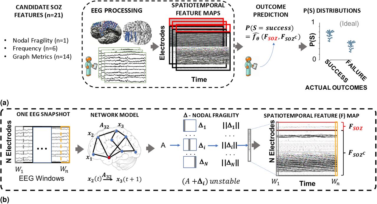
Computational experiment setup for all candidate SOZ features and statistical analysis. (a) Any candidate feature that can produce a spatiotemporal heatmap was computed from EEG data and then partitioned by the clinically annotated SOZ set and the complement, SOZC (i.e. non-SOZ electrodes) to compute a confidence statistic measuring the feature’s belief of the clinician’s hypothesis. Here FSOZ and FSOZC were the feature values within their respective sets. fθ is the function depending on the Random Forest model parameters, θ that maps the statistics of the FSOZ and FSOZC to a confidence statistic. An ideal feature would have high and low confidence for success and failed outcomes respectively. Each point on the final CS distribution comparisons represent one patient. (b) A more detailed schematic of how our proposed fragility and baseline features were computed from EEG data for a single snapshot of EEG data. See fragility methods section for description of x, A and Δ. For a similar schematic of how the baseline features were computed, see Supplemental figure S5.
6.5 Baseline features - spectral features
We constructed spectral-based features from frequency bands of interest. We applied a multi-taper Fourier transform over sliding windows of data with a window/step size of 2.5/0.5 seconds [28, 155]. We required relatively longer time windows in order to accurately estimate some of the lower frequency bands. Each EEG time series was first transformed into a 3-dimensional array (electrodes × frequency × time), and then averaged within each frequency band to form six different spectral feature representations of the data. We break down frequency bands as follows:
Delta Frequency Band [0.5 - 4 Hz]
Theta Frequency Band [4 - 8 Hz]
Alpha Frequency Band [8 - 13 Hz]
Beta Frequency Band [13 - 30 Hz]
Gamma Frequency Band [30 - 90 Hz]
High-Gamma Frequency Band [90 - 300 Hz]
HFO = R & FR [80-250 Hz & 250-500 Hz]
This resulted in a spatiotemporal heat map for each frequency band of each electrode’s spectral power over time.
6.6 Baseline features - graph analysis of networks
There are many ways to measure connectivity in iEEG data through the use of graph analysis. Specifically, we computed a time domain model using Pearson correlation (equation 1) and a frequency domain model using coherence (equation 2). We computed the connectivity matrix using MNE-Python and used the default values [135, 136]. In the equations, (i,j) are the electrode indices, Cov is the covariance, σ is the standard deviation, f is the frequency band, and G is cross-spectral density. Note that these connectivity models are attempts to capture linear correlations either in time, or in a specific frequency band, but are not dynamical system representations of the data (i.e. x(t + 1) = Ax(t)). For each network-based feature, a sliding window/step size of 2.5/0.5 seconds were used, resulting in a sequence of network matrices over time resulting in 3-dimensional arrays (electrodes × electrodes × time) [27, 28, 30].


From each network matrix, we computed the eigenvector centrality [27, 28], and the in-degree [26] features of the network for each electrode across time. Centrality describes how influential a node is within a graph network. In-degree is the weighted sum of the connections that connect to a specific node. Both features are potential measures that attempt to capture the influence of a specific electrode within an iEEG network, through the lens of graph theory. Inherently, these feature assume that the connectivity model is represented by linear correlations either in time, or a specific frequency band. We produced a spatiotemporal heat map of electrodes over time of the eigenvector centrality and the in-degree for all datasets.
6.7 Experimental design
Specifically, we tested if the neural fragility representation of the iEEG data localized the clinically annotated SOZ better compared to other proposed features, compared to clinicians and compared to chance. For fragility and all baseline features, electrodes with extreme activity deviating from the average were hypothesized as part of the SOZ. After looking at the spatiotemporal fragility heatmaps of many patients, we determined if fragility could be quantified in a way that could highlight the differences between clinical covariates such as surgical outcomes, CC, Engel class and other clinical metadata.
In order to compute a probability of successful surgical outcome for each patient, we trained a non-parametric machine learning classifier, a Random Forest classifier to output a probability value that the patient was a success. We considered a suite of hyperparameters that we then performed evaluation over a repeated nested cross-validation scheme. For each considered baseline feature we replicated the exact analysis, and we then perform statistical analysis on the final classification performance to determine the most robust feature representation.
Pooled Patient Analysis
Before we ran our quantitative comparison, we first analyzed the difference in the distributions of neural fragility between SOZ and the SOZC. We pooled all subjects together, stratified by surgical outcome and compared the neural fragility distributions using a one-sided Mann-Whitney U test (Success pvalue = 3.326e-70, and Fail pvalue = 0.355; Supplementary Figure S4). This suggested that there was some sort of an effect on average where fragility is higher in the SOZ for successful outcomes, so we next looked at the distributions per patient’s seizure snapshot around seizure onset. In Supplementary Figure S6, success outcome patients have a higher neural fragility in the SOZ. This effect is seen when pooling patients across all centers as well, where neural fragility is either i) higher before the seizure onset, or ii) has a marked difference starting at seizure onset (Supplementary Figure S7). Next, we performed a classification experiment (Figure 2) that would determine the robustness of the neural fragility representation at the patient level benchmarked against 20 other features.
Non-parametric Decision-Tree Classifier
In order to determine the value of a feature representation of the iEEG data, we posed a binary classification problem where the goal would be to determine the surgical outcome (success or failure) for a particular patient’s spatiotemporal heatmap. Each spatiotemporal heatmap was split into its SOZ and SOZC set (Fsoz and FSOZC in Figure 8). Then each set of electrodes was summarized with its quantile statistics over time, resulting in twenty signals: ten quantiles from 10-100 of the SOZ and ten quantiles of the SOZC over time. Because we do not assume any knowledge in the distribution of our proposed feature values over the SOZ and SOZC electrode sets, or over time, we use a non-parametric classifier. We used a Random Forest (RF) classifier [52]. Specifically, it was a variant known as the Structured Random Forest, or Manifold Random Forests [50, 51]. The manifold RF approach allows one to encode structural assumptions on the dataset, such as correlations in time or space of the fed in data matrix. It is apparent since each spatiotemporal heatmap represents a time series of features over time, that there are correlations along the x-axis. The input data matrix for each RF is essentially a multivariate time series that summarizes the statistics of the SOZ and SOZC over time. As a result, we obtained better results using the manifold RF because it took advantage of local correlations in time, rather than treating all values in the data matrix input as independent as done in a traditional RF model. This approach allows our classifiers to learn faster with less data, compared to treating all inputs as independent in the traditional RF model. For more information on how manifold RF improves on traditional RF, we refer readers to [50, 51]. For every model, we used the default parameters from scikit-learn and the rerf package [51, 142]. The output of the decision tree classifier is:
 where θ are the trained RF parameters and FSOZ are the heatmap values for the SOZ and Fsozc are the heatmap values for the SOZC for a specific feature representation F (shown in Supplemental Figure 8).
  is the function we are trying to estimate, which predicts the probability of successful surgical outcome for a given feature heatmap.
Hyperparameters
When looking at the iEEG data, clinicians inherently select windows of interest due to external and prior information about when the seizure clinically manifests. In this way, they look at a “period” around the seizure onset and are attempt to visually interpret the signals to be able to determine the SOZ and then as a result the region to be removed. Similarly, we consider a window of 10 seconds before seizure onset to the first 5% of the seizure event. This window was chosen apriori to analysis, and we repeated the analyses with slightly varying windows, but the results were consistent. In order to provide further contrast to the spatiotemporal heatmaps, we considered also a threshold between 0.3 and 0.7 (spaced by 0.1) that would be applied to the heatmap such that values below were set to 0. This is analagous to clinicians being able to look at a spatiotemporal heatmap and hone in only on areas that are extreme relative to the rest. If we selected this threshold per subject, then results would be meaningless, so we select a fixed threshold through nested cross-validation, where thresholds are selected on the train/validation set, and then performance is measured on the held out test set.
Structured Heatmap Input
In order to train a RF classifier, we needed to structure the spatiotemporal heatmap input. Although the previous section sets a fixed window in time, there are still a varying number of electrodes per subject due to different implantations. Thus in order to summarize the distributions of the feature values in the SOZ and SOZC sets, we convert these into a vector of 20 quantile values (10 quantiles for SOZ and 10 for SOZC), taken evenly from the 10th to the 100th quantiles. This forms a 20 × 105 data matrix per heatmap, which summarizes the SOZ and SOZC distributions over time, fixed around the seizure onset time.
Nested Cross-Validation Feature Evaluation
It is common practice when building a supervised machine learning model to incorporate cross-validation (CV) where the dataset is split into a training and testing set. However, when one has hyperparameters (in addition to the machine learning model parameters) it is necessary to control against over-fitting to the test dataset [156]. Due to our hyperparameter selection of the optimal heatmap thresholds, we used a nested CV scheme, where we split the dataset into a training, validation and a lock-box dataset, where the hyperparameters were tuned in an inner CV (70% of the dataset) with the training and validation data, and then performance was evaluated on the lock-box dataset. Note that all features were optimized separately, so that their hyperparameters were optimal for that feature. The statistic of interest here was the c-statistic known as the area under the curve (AUC). We repeated the nested-cross validation 10 times, resulting a 10-fold CV. In addition, we performed patient-level CV, ensuring that no patient was in multiple splits of the dataset (i.e. any one patient is only in the train, test, or lock-box dataset). We performed sampling with respect to clinical complexity to ensure that there was an approximately some lesional, temporal, extratemporal and multi-focal subjects in the training dataset over each CV fold. We found that this performed slightly better for all features compared to random sampling.
Statistical analysis - Hypothesis Testing
For the patient cohort, success probability values were computed from the RF classifiers trained on the spatiotemporal feature representations of the iEEG data (fragility, spectral features, and graph metrics from correlation and coherence graphs). This resulted in a distribution of probabilities for each feature. We summarize here our statistical analyses that were carried out in the above sections. When comparing distributions between two variables, we default to using the Mann-Whitney U-test [157]. In some cases, we also present results if we used the Welch’s t-test and the Likelihood Q-ratio test (LQRT), which has been shown to be more robust compared to both the Mann-Whitney U-test and t-test in the presence of noise [145, 158]. To compare the RF model performance across the 20 proposed features of fragility, spectral power and graph metrics, we used Estimation plots [144] to generate Cohen’s D effect size differences between the groups of interest, and then Mann-Whitney U tests for unpaired data, and paired Wilcoxon rank-sum tests for paired data. We corrected for any multiple comparisons using the Holm-Bonferroni step-down method [159].
We compared the success probabilities stratified by different clinical covariates: surgical outcome, Engel class, clinical complexity, handedness, gender, onset age, and surgery age. We then estimated the effect size differences between distributions in the form of a Cohen’s d statistic [160]. Cohen’s d was estimated using a non-parametric permutation test on the observed data with 5000 re-samples used to construct a 95% confidence interval [144]. The null hypothesis of our experimental setup was that the success probabilities came from the same population. The alternative hypothesis was that the populations were different (i.e. a feature could distinguish success from failed outcomes, or between different Engel classes). There is no reason to assume that our success probability distributions based on the clinical covariates are normally distributed, so we used a Likelihood Q-ratio test (LQRT), which has been shown to be more robust compared to both the Mann-Whitney U-test and t-test [145, 158]. All our statistical analyses were performed with mlxtend, pingouin, dabest, scipy and scikit-learn [139, 142–144, 146].
6.8 Feature evaluation using predicted probability of successful surgery
The fragility and all baseline features proposed generated a spatiotemporal heatmap using EEG snapshots of ictal data (outlined in Figure 8). To compare spatiotemporal heatmaps across features, we computed a probability of success (i.e. a confidence score) that is hypothesized to be high for success outcomes and low for failures for “good” features. We expected that fragility would follow a trend of decreasing confidence as CC, Engel score and ILAE score increase. For each clinical covariate group, we measured the effect size difference via bootstrapped sampling, and the statistical p-value between the distributions (see Section 6.7 for more information). We hypothesized that: i) fragility would have an effect size difference significantly different from zero when comparing success vs failed outcomes, ii) in addition, this effect size would correlate with meaningful clinical covariates, such as CC and Engel class and iii) both the effect size and p-value would be better than the proposed baseline features.
The higher the probability of success (closer to 1), the more likely the feature indicated a successful surgery, and the lower it was (closer to 0), the more likely the feature indicated a failed surgery. To compute this value, we first partition the heatmap into a SOZ and SOZC as seen in Figure 8. This forms the two sets of signals that represent the spatiotemporal feature values of the SOZ set vs the SOZC set of electrodes. Then we take windows of interest, where clinicians find most valuable for SOZ localization: the period before seizure and right after seizure onset, and performing a nested CV of RF models. The efficacy of each proposed feature is evaluated based on how well the trained RF model is able to predict the surgical outcomes. We tested our hypotheses stated above by computing a probability of success from each feature heatmap for each patient, and estimated the distribution differences of the CS between various clinical covariates.
6.9 spatiotemporal feature heatmap interpretability
We next addressed two questions: i) are the success probability values interpretable? and ii) can we parse out which statistics of the SOZ and SOZC were relevant to predicting surgical outcome?
In order to determine how valid the output probability values are, we first computed a calibration curve, which told us how well-calibrated the probability values were [161]. We furthermore compared the calibration curves across neural fragility, spectral features and graph metrics. With relatively good discrimination measured by the AUC and good calibration, we were able to then compare the CS across specific clinical covariates. We specifically compared the probability values when stratified by clinical complexity (CC) scores, Engel scores and ILAE scores. Since epilepsy and reasons for failed surgeries are so complex, these are clinical methods for stratifying patient groups based on observed etiology. We analyzed how the success probability differs across each of these categories. In addition, we looked at how the success probabilities might differ across other clinical variables, such as sex (M vs F), handedness (R vs L), epilepsy onset age (years), and age during surgery (years).
Qualitatively reading off a spatiotemporal heatmap is highly interpretable as one can match raw iEEG segments to certain time periods in the heatmap. In terms of the quantitative evaluation, the RF machine learning model is also highly interpretable. For every patient, the time-varying quantile signals (from 10th to the 100th) of the SOZ and SOZC were computed for every iEEG heatmap, as specified in Section 6.7. We used permutations feature importance sampling to obtain a relative weighting of each signal over time and how important it was in allowing the RF to correctly determine surgical outcome. This was visualized as a heatmap showing the mean and std importance scores of the SOZ and SOZC statistics, as shown in Supplemental Figure S11.
In addition, we claim that human interpretability of the spatiotemporal heatmap relies on contrast between the SOZ and SOZC regions in successful outcomes. For every heatmap, we computed an interpretability ratio, which was defined as:
 where I is the interpretability ratio for a specific subject’s feature heatmap F. Fsoz(90th) is the 90th quantile and up feature values of the SOZ, and Fsozc (90th) is for the SOZC. This ratio is then stratified according to surgical outcome, which we expect higher ratios for successful outcomes and lower ratios for failed outcomes. We quantified this difference using Cohen’s D effect size and Mann Whitney U-test Pvalues (see Methods 6.7).
6.10 Code and data availability
All code related to generate the figures are at https://github.com/adam2392/fragility_in_ieeg (will be made public once published). We include a jupyter notebook written in Python to help reproduce figures. We also released the raw iEEG data for patients from NIH, UMH, UMMC, and JHH in the OpenNeuro repository in the form of BIDS-iEEG (https://openneuro.org/datasets/ds003029). Due to restrictions on data sharing fromCClinic, we were unable to release the raw iEEG data that we received from this site.
7 Supplementary Material
We include in the supplementary section, also a “lessons-learned” summary of how to proceed with preprocessing iEEG data and reasons why. In addition, raw data is present in the link in Section 6.1. Any supplementary Information and Source Data files are available in the online version of the paper.
7.1 Dataset and definition elaborations

After non-invasive analysis is inconclusive, a complex and relatively lengthy iEEG workflow for localization takes place. During invasive monitoring, clinicians identify the clinically hypothesized SOZ as the electrodes with the earliest visually identifiable EEG signatures at seizure onset (see [47] for a review of this process). Note it is impossible to observe the EZ directly, so clinicians are required to estimate where to place iEEG electrodes and then successfully interpret the network patterns and raw iEEG patterns (e.g. HFOs, or spiking activity) to formulate the clinical SOZ hypothesis. An estimate of the true EZ is then created using a combination of the clinical SOZ hypothesis, as well non-invasive findings. When possible, subsequent surgical resection or laser ablation, generally including the SOZ along with a variable extent of additional tissue, is performed. Post-operatively, patients are followed for 12+ months and categorized as either success, or failure as defined in Section 6.1. This translates to clinical outcomes measured by Engel score, or ILAE score. As a result of seizure freedom, one can assume that the clinical SOZ included the EZ in some manner. In contrast, if seizures continue, then the clinical SOZ was not sufficient to cover the EZ.

Distributions of the 91 patient dataset based on a variety of clinical factors, such as gender (a), handedness (b), clinical complexity (c), and Engel class (d). The plots show distributions over the 91 patients used in analysis.

To build quantitative intuition on what neural fragility means in the context of a dynamical iEEG system, we construct a 2-node EEG network example with an excitatory (E) and inhibitory (I) population of neurons. For a qualitative description, see Figure 1. xI(t) and xE(t) are the EEG activity of the I and E neuronal population respectively. ‘A’ is a linear network model quantifying how each population affects the rest over time. Δ (i.e. the fragility), is the amount of change added to a node’s connections. The fragility of the node is quantified as the minimal amount of change necessary to cause seizure-like phenomena. (a) shows a stable network without a perturbation added, such that the network responses due to an impulse at I result in a transient that reverts to baseline. (b) shows a perturbation added, but the network is still stable with a slightly larger transient when an impulse is applied to node I. Then (c) shows enough of a perturbation is added, such that the network becomes unstable; an impulse applied at node I results in oscillatory activity that does not quickly return to baseline. The magnitude of the Δ added in (c) is the fragility of node I.

Pooled fragility distribution analysis for all 91 subjects: failed (a), no surgery (b) and successful surgery (c) datasets. Each SOZ (soz in blue bars) and SOZC (‘nsoz’ in orange bars) distribution per patient was bootstrap sampled (see Methods section for more information on sampling) and then compared using the one-sided Mann-Whitney U test. The corresponding test yielded a statistic of 2776334 (PValue = 0.355) for the failed patient outcomes and a statistic of 36836739 (PValue = 3.326e-70) for the successful patient outcomes. The patients without resection were not included in the analysis comparing to outcome, but these patients can present as interesting case studies where the SOZ was hypothetically localizable, but perhaps was too close to eloquent areas.

An accompanying schematic for Figure 8, describing how we processed baseline features, such as spectral power, and graph metrics. The feature heatmap processing is exactly the same as fragility, allowing us to compare the feature representations of neural fragility, spectral power and graph metrics of correlation and coherence derived graphs for the purposes of SOZ localization.
7.2 Pooled subject and SOZ vs SOZC analysis

Red SOZ vs black SOZC signals for patients presented in Figure 3: Patient_01 (a), Patient_26 (b), Patient_40 (c). For each patient, the ictal snapshots available are visualized around seizure onset with 5 seconds before onset until the first 20% of the seizure. Note that not necessarily all electrodes in the clinically annotated SOZ are part of the EZ when the patient had a successful outcome. Therefore, if neural fragility had value in contrasting true EZ electrodes from non-EZ electrodes, then any extra electrodes clinically annotated in the SOZ should have relative lower fragility.

Red SOZ vs black SOZC fragility signals for pooled patients within each of the five centers with successful (a) and failed outcomes (b) for NIH (n=14), JHH (n=4), CC (n=61), UMH (n=5), and UMMC (n=7) (top to bottom respectively). Note UMMC only had successful outcomes, so there was no curve for the failures. Seizure periods were resampled and normalized to 100 samples for averaging and viewing purposes. In JHH and UMH, there were only one and two patients in successful outcomes respectively.
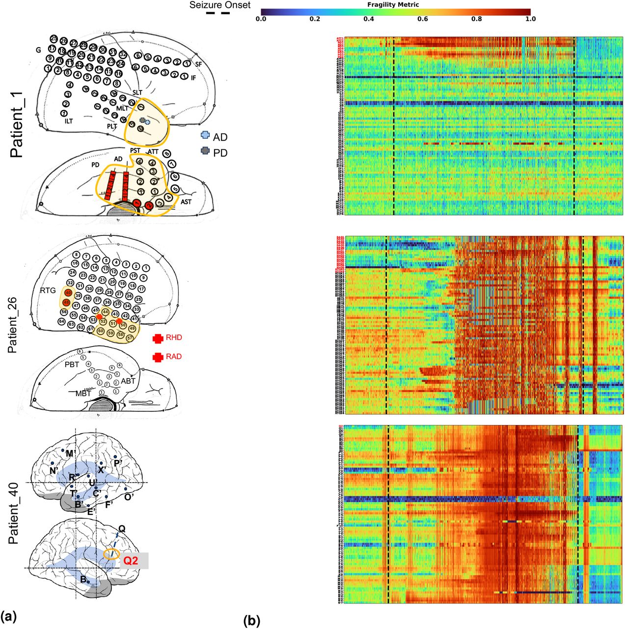
Fragility heatmaps with electrodes on y-axis and time on x-axis with the dashed white-lines denoting seizure onset and offset. Shows a period of 30 seconds before seizure onset and 30 seconds after seizure offset. (a) Shows clinically annotated maps of the implanted ECoG/SEEG electrodes with red denoting SOZ contacts. (b) shows spatiotemporal fragility heatmaps for example of successful outcome (Patient_01), and failed outcome (Patient_26 and Patient_40). The color scale represents the amplitude of the normalized fragility metric, with closer to 1 denoting fragile regions and closer to 0 denoting relatively stable regions. The contacts in red and orange are part of the SOZ and RZ, respectively as defined in Methods section. Note that the red contacts are also part of the RZ. Visualized with Turbo continuous colormap. Best seen if viewed in color.

Calibration curve showing the fraction of actual successful surgical outcomes on the y-axis vs the average CS output on the x-axis. This curve measures how calibrated the predicted success probability values are to the true risk stratification of the patient population. The closer a curve is to the y = x line, then the more calibrated a model is. It is quantified by the Brier-loss (closer to 0 is better), which is shown in the legend, and is significantly lower then the next best feature (an improvement of 15%).

(a) The ROC curve over 10 folds of cross-validation of the held-out test set obtained by applying a Random Forest model onto the spatiotemporal heatmaps to predict surgical outcome (See 6 Section). Fragility and the top-3 baseline features in terms of AUC are visualized. The shaded area represents the standard deviation of the curve obtained by linear interpolation for visualization purposes. The AUC of fragility obtained a 0.88 ± 0.064 over the 10 standard deviation with a relative improvement of 7.2% improvement in AUC compared to the next best feature representation (i.e. the beta frequency band). At the Youden point (stars), neural fragility obtains a balanced accuracy score of 0.76 ± 0.06, and an improvement of 0.32 in TPR and 0.32 in FPR compared to the clinical operating point (red star). (c) A paired estimation plot showing how the same test set of patients differed in AUC depending on whether it was using the fragility, or beta feature heatmap representation. The paired Cohen’s D effect size was computed at −0.975 (−1.97 to −0.29; 95% CI). The p-values associated with the difference between Neural Fragility and the Beta frequency band were 0.0204, 0.0273, and 0.0225 using the Wilcoxon rank-sum test, permutation test, and the paired student t-test respectively. Comparing Fragility to all other feature representations were more different in terms of larger effect sizes and smaller p-values.

Estimated feature importance (mean and stdev) of the associated fragility heatmap used estimated using permutation. The metric of interest was the concordance statistic (i.e. AUC) of the ROC curve. The original feature map is transformed into a 20-dimensional set of time-varying statistics of its SOZ and SOZC electrodes describing the quantiles of the spatiotemporal heatmap (10% - 100% quantiles). This time-varying summary allows these heatmaps to be pooled together across subjects when training a Random Forest classifier as described in Section 6.

Fragility success probabilities split by clinical factors, such as handedness (a), gender (b), onset age (c) and age at surgery (d). Effect sizes were estimated using the permutation test and Mann Whitney U test described in section 6. The corresponding effect sizes and p-values were (0.1/0.99) for handedness, and (0.12/0.7) for gender. The slopes were all negligibly close to 0 for onset age and surgery age linear fit. Note that not all patients had data for each of these categories, so the subset of available data was used.

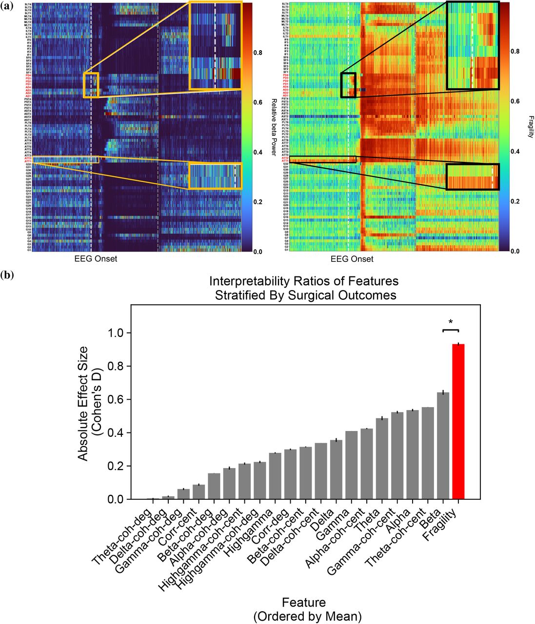
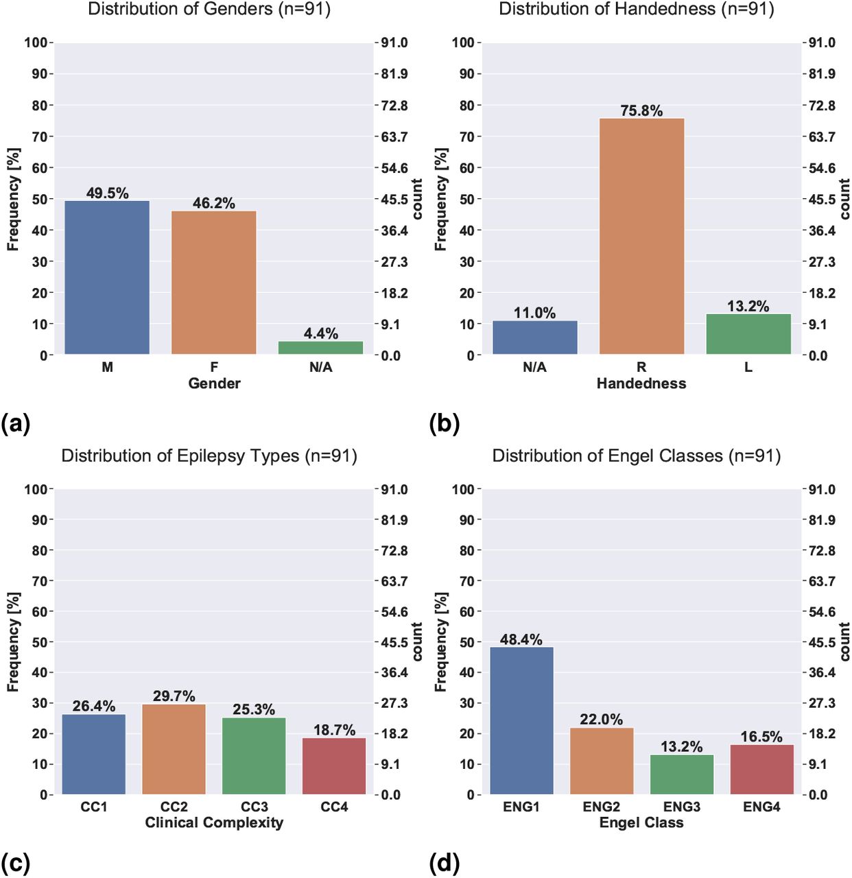
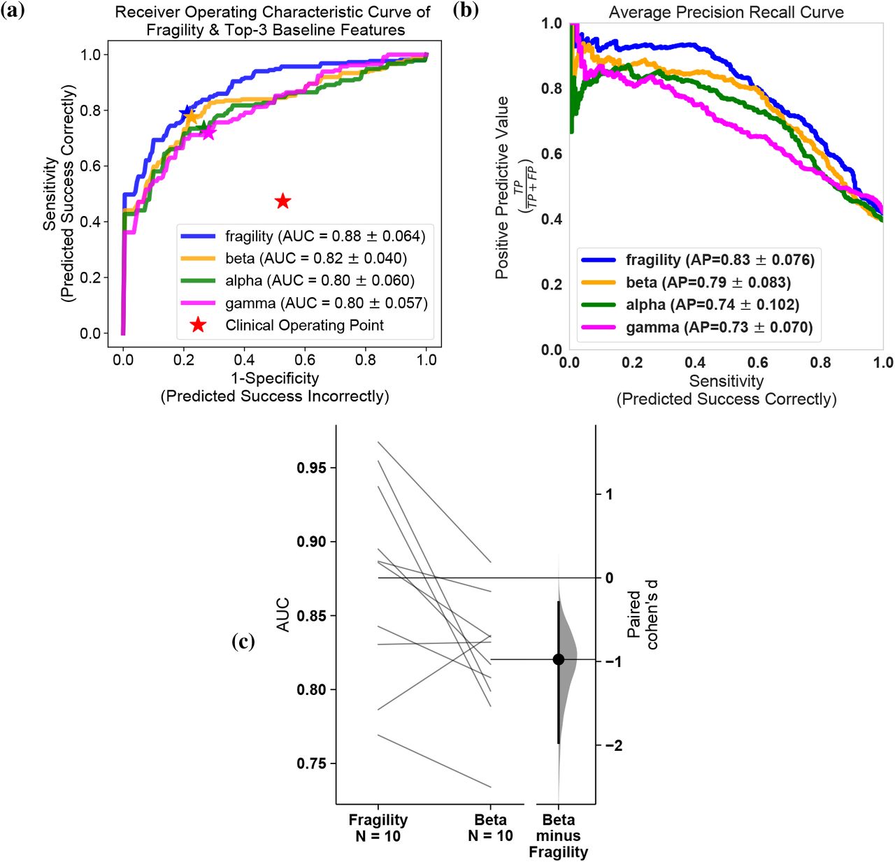
Fragility versus frequency power in the delta, theta, alpha, beta, gamma and highgamma band for Patient_01, Patient_26, and Patient_40. For band definitions, refer to Section 6.5. Every point represents the spectral power and neural fragility value from a randomly chosen window and electrode from one of the subjects. No significant correlation is seen or computed from the data. Each spectral feature and fragility are normalized as described in Section 6.
4 Acknowledgements
AL is supported by NIH T32 EB003383, the NSF GRFP (DGE-1746891), the Arcs Scholarship, Whitaker Fellowship and the Chateaubriand Fellowship. SVS is supported by NIH R21 NS103113, the Coulter Foundation, Maryland Innovation Initiative, US NSF Career Award 1055560 and the Burroughs Wellcome Fund CASI Award 1007274. Computational resources were also provided by the Maryland Advanced Research Computing Center (MARCC). The authors would like to thank Carey Priebe for useful discussions on statistical analyses, Joshua Vogelstein for introducing AL to the concepts of Structured Random Forests, Sarah Kim and Rachel June Smith for helpful reviews of the manuscript and Macauley Breault for help in creating brain figures.
Footnotes
↵* Co-senior authors
Adding a classification experiment (using a Structured Random Forest) to better parse out the effect differences between feature representations. Improved the presentation of the results and figures, and included an interpretability section. Improved literature review.
1 Also reachable at adam2392 at gmail dot com. Also reachable at the NCSL website: https://sarmalab.icm.jhu.edu/. Department of Biomedical Engineering, Johns Hopkins University, Baltimore, MD, 21218
References
- [1].↵
- [2].
- [3].
- [4].
- [5].↵
- [6].↵
- [7].↵
- [8].↵
- [9].↵
- [10].
- [11].↵
- [12].↵
- [13].↵
- [14].
- [15].↵
- [16].↵
- [17].↵
- [18].
- [19].↵
- [20].
- [21].↵
- [22].
- [23].↵
- [24].↵
- [25].↵
- [26].↵
- [27].↵
- [28].↵
- [29].
- [30].↵
- [31].↵
- [32].
- [33].
- [34].
- [35].↵
- [36].↵
- [37].↵
- [38].↵
- [39].↵
- [40].
- [41].↵
- [42].↵
- [43].
- [44].↵
- [45].↵
- [46].↵
- [47].↵
- [48].↵
- [49].↵
- [50].↵
- [51].↵
- [52].↵
- [53].↵
- [54].↵
- [55].↵
- [56].
- [57].
- [58].↵
- [59].↵
- [60].
- [61].↵
- [62].↵
- [63].↵
- [64].↵
- [65].↵
- [66].↵
- [67].↵
- [68].↵
- [69].↵
- [70].↵
- [71].↵
- [72].↵
- [73].
- [74].↵
- [75].
- [76].
- [77].
- [78].
- [79].
- [80].↵
- [81].
- [82].
- [83].
- [84].↵
- [85].↵
- [86].↵
- [87].↵
- [88].
- [89].
- [90].
- [91].
- [92].
- [93].
- [94].
- [95].
- [96].
- [97].↵
- [98].↵
- [99].↵
- [100].
- [101].
- [102].↵
- [103].↵
- [104].
- [105].
- [106].
- [107].↵
- [108].↵
- [109].↵
- [110].↵
- [111].↵
- [112].↵
- [113].↵
- [114].↵
- [115].↵
- [116].↵
- [117].↵
- [118].
- [119].
- [120].
- [121].
- [122].
- [123].
- [124].↵
- [125].↵
- [126].↵
- [127].↵
- [128].↵
- [129].
- [130].↵
- [131].↵
- [132].↵
- [133].↵
- [134].
- [135].↵
- [136].↵
- [137].
- [138].
- [139].↵
- [140].↵
- [141].↵
- [142].↵
- [143].
- [144].↵
- [145].↵
- [146].↵
- [147].↵
- [148].
- [149].↵
- [150].↵
- [151].↵
- [152].↵
- [153].↵
- [154].↵
- [155].↵
- [156].↵
- [157].↵
- [158].↵
- [159].↵
- [160].↵
- [161].↵


