


Abstract
Biomarker use in exposure assessment is increasingly common, and consideration of related issues is of growing importance. Exposure quantification may be compromised when measurement is subject to a lower threshold. Statistical modeling of such data requires a decision regarding the handling of such readings. Various authors have considered this problem. In the context of linear regression analysis, Richardson and Ciampi (Am J Epidemiol 2003;157:355–63) proposed replacement of data below a threshold by a constant equal to the expectation for such data to yield unbiased estimates. Use of such an imputation has some limitations; distributional assumptions are required, and bias reduction in estimation of regression parameters is asymptotic, thereby presenting concerns about small studies. In this paper, the authors propose distribution-free methods for managing values below detection limits and evaluate the biases that may result when exposure measurement is constrained by a lower threshold. The authors utilize an analytical approach and a simulation study to assess the effects of the proposed replacement method on estimates. These results may inform decisions regarding analytical plans for future studies and provide a possible explanation for some amount of the discordance seen in extant literature.
The growing use of biomarkers in exposure assessment suggests the need to address issues related to their measurement. Even when levels are sufficient for measurement, some random exposure measurement error is expected, in part related to instrument precision. However, in many cases a proportion of study participants have levels at or below some experimentally determined detection limit (dl). Investigators are often interested in the risk of negative health outcomes associated with such levels. For example, studies of serum organochlorine levels, lipophilic xenobiotics, and breast cancer have determined that up to 99 percent of study participants have levels below the dl for some toxicants under study (1).
Biomarker quantification may be compromised if instrumentation cannot detect low levels. This may occur, for example, in quantitation of immunoassays (e.g., enzyme-linked immunosorbent assays) that require antigen concentrations sufficient for binding by antibodies. Highly specific binding conditions may impair antibody sensitivity and thereby challenge quantitation of low levels (2). Alternatively, assays may detect low biomarker levels but suffer from insufficient specificity, and measurement of exposure is hampered by background. The detection limit is often determined as a function of observed variance for a series of blanks; the terms “limit of detection” and “limit of quantification” generally correspond to three and 10, respectively, standard deviations from serial measurement of blanks (3). As such, numerical data are observable above and below the dl; even among values above the threshold, it may not be possible to clearly delineate between those that are “real” and those that are not. Data below the threshold are often reported by laboratories as “nondetects,” and the data analyst or epidemiologist is limited to this qualitative assessment.
Statistical modeling of these data requires decisions regarding their handling (4, 5). Conventional approaches include omission, resulting in a truncated data set, and imputation with a constant, such as the dl or a fraction thereof (e.g., dl/2, dl/√2); or the observed values may be used directly or indirectly (4–7). Many of these imputations have their origins in well-behaved distributions, such as normal (in the case of dl/2) and lognormal (in the case of dl/√2), and will yield correct inferences if these distributional assumptions are not grossly violated. Lubin et al. (5) propose a multiple imputation approach to handling nondetects when the exposure distribution can be assumed. Richardson and Ciampi (7) developed a coefficient of bias to linear regression coefficient estimates when exposure is measured with a detection threshold and random error, and they proposed replacement of below-threshold data by the expectation for such data (i.e., E[x|x < dl]) to yield unbiased estimates. Application of this theory to practice also requires investigators to assume an exposure distribution function. In contrast to these approaches, there has been comparatively little attention toward implicitly and explicitly nonparametric approaches to measurement with a threshold.
In this paper, the authors propose distribution-free methods for managing values below the dl and evaluate biases that result when exposure measurement is constrained by a lower threshold. Results from an analytical approach and those of a simulation study assessing the proposed replacement method are described. The proposed method allows investigators to relax the assumptions (e.g., distributional, asymptotic) necessary for use of other approaches. These results may inform decisions by investigators regarding appropriate analytical plans for future studies and provide a possible explanation for the discordance seen in current literature.
STATEMENT OF THE PROBLEM AND ANALYTICAL SOLUTION
In this paper, least-squares estimation was used to determine an a that may be used in place of censored data for unbiased estimation of regression parameters. Nonnumerical and numerical instrument responses for below-threshold measurements were addressed. Additionally, the circumstances of instrument noise bounded by the detection limit (where the probability of values above the limit being due to error alone is approximately zero) and unbounded (where values above the limit will be a mix of noise alone and signal) were considered. We apply the contexts of linear regression models with both known and unknown intercepts and, additionally, provide an extension for application to logistic regression models.
Nonnumerical indicator below the detection limit
No intercept, α, models (condition 1A).
Models that estimate the intercept, α (condition 1B).
Numerical noise below the limit of detection
Whereas the previous sections concerned the instrumentation response of “ND,” numerical information may be available for data below dl. Importantly, if detection limit error is known to be less than the dl itself (ξ is reasonably bounded by the dl), observations below dl may be identified as such, and this becomes a special case of section 1. In this case, investigators may follow the previously discussed methodologies for models with or without intercept.
When ξ is unknown or is known to have greater magnitude than dl, the observations due to noise cannot be easily identified; the zi are observed both above and below dl for all individuals, and those with detection limit error are not easily discernible from those free of this error. Formally, suppose Pr(ξ > dl) > 0. Under the described scenario of detection limit error, this may be the case if the detection limit is set as two, rather than three (limit of detection) or 10 (limit of quantification) standard deviations of noise. In this circumstance, there is no simple approach to determining an optimal imputation; however, numerical approaches for models both with and without intercept are shown in appendix 3.
Alternatively, detection limits are occasionally determined solely on the basis of the distribution of additive random error (or concurrent detection of some contaminant). Consider true exposure, x, and all concurrently detected others, ω; all samples may be reasonably thought of as the sum of these two components (i.e., x + ω). When all levels of x are subject to the same source of error, which is independent of x, then the proposed imputations remain valid; however, alternatively, the observed values may be used for analysis in combination with commonly used methods for handling random measurement error (10, 11).
MOTIVATING EXAMPLE
We consider the association between total cholesterol and serum vitamin E in a healthy population using a population-based sample of randomly selected residents aged 35–79 years who lived in two counties in western New York State. After exclusions, a total of 857 men and women were selected for analysis. Blood specimens were analyzed for routine chemistry, hematology, and a number of chronic disease and nutritional factors, as well as serum vitamin E levels.
For cholesterol and vitamin E, all observations were measured above the dl. Regression analysis suggests a linear association between serum cholesterol and serum vitamin E (
To this end, estimates were compared from linear regression of serum cholesterol on serum vitamin E. For exposure data, these models used one of the four following options: 1) all available exposure data (“gold standard”); 2) replacement of all data below the imposed threshold with the mean level of vitamin E of all data below the threshold; 3) the mean of all data above the threshold; or 4) zero. Importantly, the second circumstance relies on distributional assumptions that would be unverifiable under a true detection limit. Models were run for the known intercept as well as for estimation of the intercept.
Table 1 displays results of the known intercept regression. Replacement of subthreshold data by the average of subthreshold data yielded estimates almost identical to those when all data were used. However, under usual conditions, direct calculation of this quantity is not possible, and it must be estimated assuming some distribution. Conversely, replacement by zero requires no such assumptions and resulted in estimates not statistically different from those under the ideal scenario of no threshold. Table 2 displays results of linear regression models estimating both slope and intercept. Use of the proposed average of above-threshold data for replacement of missing data yielded good estimates of parameters, both intercept and slope. As with the use of zero for no-intercept models, use of this imputation for estimation is nonparametric and requires no distributional knowledge. Moreover, estimates of slope were hampered by slight departures from the assumptions of linear regression of the data. Use of zero for replacement of missing data resulted in estimates statistically different from those under no constraint by a detection threshold.
Coefficient estimates from linear regression with a known intercept of serum cholesterol on serum vitamin E, with values below the limit of detection replaced by the average (x|x < dl*) and zero
All values (reference) | Replace by average (x|x < dl) | Replace by zero | |
|---|---|---|---|
\(\mathrm{{\hat{{\beta}}}}\) | 4.07 | 4.06 | 4.19 |
| SE* \((\mathrm{{\hat{{\beta}}}})\) | 0.14 | 0.14 | 0.15 |
| 95% CI* \((\mathrm{{\hat{{\beta}}}})\) | 3.80, 4.34 | 3.79, 4.33 | 3.90, 4.48 |
All values (reference) | Replace by average (x|x < dl) | Replace by zero | |
|---|---|---|---|
\(\mathrm{{\hat{{\beta}}}}\) | 4.07 | 4.06 | 4.19 |
| SE* \((\mathrm{{\hat{{\beta}}}})\) | 0.14 | 0.14 | 0.15 |
| 95% CI* \((\mathrm{{\hat{{\beta}}}})\) | 3.80, 4.34 | 3.79, 4.33 | 3.90, 4.48 |
dl, detection limit; SE, standard error; CI, confidence interval.
Coefficient estimates from linear regression of serum cholesterol on serum vitamin E, with values below the limit of detection replaced by the average (x|x < dl*), average (x|x > dl), and zero
All values (reference) | Replace by average (x|x < dl) | Replace by average (x|x > dl) | Replace by zero | |
|---|---|---|---|---|
\(\mathrm{{\hat{{\alpha}}}}\) | 196.88 | 197.39 | 204.53 | 219.76 |
| SE* \((\mathrm{{\hat{{\alpha}}}})\) | 5.21 | 5.26 | 7.51 | 3.35 |
| 95% CI* \((\mathrm{{\hat{{\alpha}}}})\) | 186.67, 207.09 | 187.08, 207.7 | 189.81, 219.25 | 213.19, 226.33 |
\(\mathrm{{\hat{{\beta}}}}\) | 4.07 | 4.03 | 3.02 | 2.89 |
| SE \((\mathrm{{\hat{{\beta}}}})\) | 0.36 | 0.36 | 0.46 | 0.24 |
| 95% CI \((\mathrm{{\hat{{\beta}}}})\) | 3.36, 4.78 | 3.32, 4.74 | 2.12, 3.92 | 2.42, 3.36 |
dl, detection limit; SE, standard error; CI, confidence interval.
LOGISTIC REGRESSION
Frequently, investigators face exposure measurement thresholds when investigating binary outcomes (e.g., presence or absence of disease) using logistic regression models for evaluation of risk. These models are often used for analysis of case-control study data. In this context, investigators rarely have an interest in intercept estimates, interpretation of which is generally meaningless (9). In such situations, the discussion for condition 1A is applicable, and bias is minimized when a equals zero. This is shown empirically in a simulation study described in the next section. A more detailed discussion and proof are shown in appendices 4 and 5.
The solution under maximum likelihood estimation is complicated, even with known intercept. When the intercept is unknown, solutions to two nonlinear equations are required (appendix 5). A solution can be determined only in rare cases and where strong assumptions regarding the observed data are used and where the proposed methodology is applied. However, this problem is beyond the scope of this paper.
MONTE CARLO SIMULATION STUDY
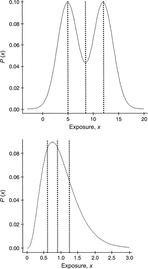
Probability distribution functions for Monte Carlo simulation study: exposure-distributed bimodal normal (top) and gamma (bottom). Dotted lines indicate the values utilized for the threshold corresponding to the 25th, 50th, and 75th percentiles.
Table 3 displays the simulated Monte Carlo variance of the maximum likelihood estimator
β | d | x < dl (%) | Bias (Monte Carlo estimator of β) | Variance (Monte Carlo estimator of β) | ||||||||||||
|---|---|---|---|---|---|---|---|---|---|---|---|---|---|---|---|---|
| a = | a = | |||||||||||||||
| 0 | E(x|x < d) | dl | dl/2 | 0 | E(x|x < d) | dl | dl/2 | |||||||||
| 0.3 | 5 | 25 | 0.00026 | 0.00019 | 0.00117 | 0.00057 | 0.00025 | 0.00025 | 0.00027 | 0.00026 | ||||||
| 8.5 | 50 | 0.00068 | 0.00059 | 0.01407 | −0.00082 | 0.00026 | 0.00025 | 0.00043 | 0.00026 | |||||||
| 12 | 75 | 0.00117 | −0.00796 | 0.05360 | 0.00197 | 0.00039 | 0.00038 | 0.00307 | 0.00046 | |||||||
| 0.5 | 5 | 25 | −0.00045 | −0.00075 | 0.00276 | −0.00127 | 0.00024 | 0.00024 | 0.00024 | 0.00024 | ||||||
| 8.5 | 50 | −0.00062 | −0.00518 | 0.04611 | −0.00833 | 0.00028 | 0.00031 | 0.00225 | 0.00037 | |||||||
| 12 | 75 | −0.00183 | −0.04409 | 0.12608 | −0.08398 | 0.00068 | 0.00239 | 0.01598 | 0.00794 | |||||||
| 0.7 | 5 | 25 | −0.00230 | −0.00476 | 0.01814 | −0.00807 | 0.00068 | 0.00068 | 0.00078 | 0.00077 | ||||||
| 8.5 | 50 | 0.00668 | −0.03878 | 0.14702 | −0.09131 | 0.00160 | 0.00253 | 0.02174 | 0.02174 | |||||||
| 12 | 75 | −0.12120 | −0.07991 | 0.26264 | 0.14123 | 0.10959 | 0.07712 | 0.16906 | 0.14076 | |||||||
dl, detection limit.
Values of E(x|x < d) are as follows: 3.405 for d = 5; 4.934 for d = 8.5; 6.700 for d = 12. P{Yi = 1|xi} = (1 + exp(−c − βxi))−1, where c = −5, c is known, and xi = N(5, 22)(1−θi) + N(12, 22)θi, where θi, i ≥ 1 are independent, identically Bernoulli-distributed random variables with P{θi = 1} = 1/2.
β | d | x < dl (%) | Bias (Monte Carlo estimator of β) | Variance (Monte Carlo estimator of β) | ||||||||||||
|---|---|---|---|---|---|---|---|---|---|---|---|---|---|---|---|---|
| a = | a = | |||||||||||||||
| 0 | E(x|x < d) | dl | dl/2 | 0 | E(x|x < d) | dl | dl/2 | |||||||||
| 0.3 | 5 | 25 | 0.00026 | 0.00019 | 0.00117 | 0.00057 | 0.00025 | 0.00025 | 0.00027 | 0.00026 | ||||||
| 8.5 | 50 | 0.00068 | 0.00059 | 0.01407 | −0.00082 | 0.00026 | 0.00025 | 0.00043 | 0.00026 | |||||||
| 12 | 75 | 0.00117 | −0.00796 | 0.05360 | 0.00197 | 0.00039 | 0.00038 | 0.00307 | 0.00046 | |||||||
| 0.5 | 5 | 25 | −0.00045 | −0.00075 | 0.00276 | −0.00127 | 0.00024 | 0.00024 | 0.00024 | 0.00024 | ||||||
| 8.5 | 50 | −0.00062 | −0.00518 | 0.04611 | −0.00833 | 0.00028 | 0.00031 | 0.00225 | 0.00037 | |||||||
| 12 | 75 | −0.00183 | −0.04409 | 0.12608 | −0.08398 | 0.00068 | 0.00239 | 0.01598 | 0.00794 | |||||||
| 0.7 | 5 | 25 | −0.00230 | −0.00476 | 0.01814 | −0.00807 | 0.00068 | 0.00068 | 0.00078 | 0.00077 | ||||||
| 8.5 | 50 | 0.00668 | −0.03878 | 0.14702 | −0.09131 | 0.00160 | 0.00253 | 0.02174 | 0.02174 | |||||||
| 12 | 75 | −0.12120 | −0.07991 | 0.26264 | 0.14123 | 0.10959 | 0.07712 | 0.16906 | 0.14076 | |||||||
dl, detection limit.
Values of E(x|x < d) are as follows: 3.405 for d = 5; 4.934 for d = 8.5; 6.700 for d = 12. P{Yi = 1|xi} = (1 + exp(−c − βxi))−1, where c = −5, c is known, and xi = N(5, 22)(1−θi) + N(12, 22)θi, where θi, i ≥ 1 are independent, identically Bernoulli-distributed random variables with P{θi = 1} = 1/2.
β | d | x < dl (%) | Bias (Monte Carlo estimator of β) | Variance (Monte Carlo estimator of β) | ||||||||||||
|---|---|---|---|---|---|---|---|---|---|---|---|---|---|---|---|---|
| a = | a = | |||||||||||||||
| 0 | E(x|x < d) | dl | dl/2 | 0 | E(x|x < d) | dl | dl/2 | |||||||||
| 0.3 | 0.634 | 25 | 0.00153 | 0.00148 | 0.00730 | −0.00165 | 0.01204 | 0.01148 | 0.01412 | 0.01373 | ||||||
| 0.919 | 50 | 0.00309 | 0.00280 | 0.02926 | −0.00595 | 0.01373 | 0.01269 | 0.01580 | 0.01450 | |||||||
| 1.278 | 75 | 0.00708 | 0.00586 | 0.07383 | −0.01368 | 0.01384 | 0.01289 | 0.01628 | 0.01474 | |||||||
| 1.5 | 0.634 | 25 | −0.00427 | −0.00405 | 0.04319 | −0.02375 | 0.01636 | 0.01582 | 0.01699 | 0.01732 | ||||||
| 0.919 | 50 | −0.00630 | −0.00599 | 0.18292 | −0.07987 | 0.01933 | 0.01590 | 0.04408 | 0.02821 | |||||||
| 1.278 | 75 | −0.01079 | 0.00085 | 0.42685 | −0.14473 | 0.02450 | 0.01982 | 0.18934 | 0.04348 | |||||||
dl, detection limit.
Values of E(x|x < d) are as follows: 0.454 for d = 0.634; 0.615 for d = 0.919; 0.772 for d = 1.278. P{Yi = 1|xi} = (1 + exp(−c − βxi))−1, where c = −1, c is known, and xi ∼ gamma(shape = 4, scale = 4).
β | d | x < dl (%) | Bias (Monte Carlo estimator of β) | Variance (Monte Carlo estimator of β) | ||||||||||||
|---|---|---|---|---|---|---|---|---|---|---|---|---|---|---|---|---|
| a = | a = | |||||||||||||||
| 0 | E(x|x < d) | dl | dl/2 | 0 | E(x|x < d) | dl | dl/2 | |||||||||
| 0.3 | 0.634 | 25 | 0.00153 | 0.00148 | 0.00730 | −0.00165 | 0.01204 | 0.01148 | 0.01412 | 0.01373 | ||||||
| 0.919 | 50 | 0.00309 | 0.00280 | 0.02926 | −0.00595 | 0.01373 | 0.01269 | 0.01580 | 0.01450 | |||||||
| 1.278 | 75 | 0.00708 | 0.00586 | 0.07383 | −0.01368 | 0.01384 | 0.01289 | 0.01628 | 0.01474 | |||||||
| 1.5 | 0.634 | 25 | −0.00427 | −0.00405 | 0.04319 | −0.02375 | 0.01636 | 0.01582 | 0.01699 | 0.01732 | ||||||
| 0.919 | 50 | −0.00630 | −0.00599 | 0.18292 | −0.07987 | 0.01933 | 0.01590 | 0.04408 | 0.02821 | |||||||
| 1.278 | 75 | −0.01079 | 0.00085 | 0.42685 | −0.14473 | 0.02450 | 0.01982 | 0.18934 | 0.04348 | |||||||
dl, detection limit.
Values of E(x|x < d) are as follows: 0.454 for d = 0.634; 0.615 for d = 0.919; 0.772 for d = 1.278. P{Yi = 1|xi} = (1 + exp(−c − βxi))−1, where c = −1, c is known, and xi ∼ gamma(shape = 4, scale = 4).
DISCUSSION
We have considered analysis of exposures subject to a lower threshold, a circumstance frequently confronted in epidemiologic studies evaluating relations between laboratory data and health outcomes. Appropriate management of data below such a threshold is imperative for proper conclusions, and available information may not be sufficient for use of parametric approaches. By use of an analytical approach to finding unbiased estimators, substitution of zero for subthreshold/missing data was observed to minimize bias when using no/known intercept linear regression models; when estimating the intercept, imputation of the average of data above detection limits yielded optimal estimates. Data from a population-based study were used to display the effects of the proposed solutions. Additionally, Monte Carlo simulations were used to demonstrate solutions applied to logistic regression where the intercept is known and/or excluded from models, which is appropriate for case-control study data. Imputation of zero performed optimally in these circumstances.
While this result may seem illogical, the solutions for linear regression may be understood intuitively. Imputation of zero for exposure values below detection limits essentially eliminates the leverage of those data on estimation when concerned solely with the slope of the regression line (i.e., the no-intercept model). If the data perfectly meet the assumptions for this model, then use of the subset of data above the threshold will yield estimates identical to those produced using all the data when they are not subject to a threshold. Similarly, imputation of the expected value for all observed data (i.e., z > dl) eliminates the leverage of those data points on estimation of the regression line slope while also allowing for estimation of the intercept; imputation of zero clearly has implications for estimation of the linear regression intercept.
The real data example results display the effectiveness of these imputations as well as certain limitations. Estimates under the proposed imputations were not statistically different from those subjected to no detection threshold nor were they identical. In combination with normal sampling variability, when data do not perfectly conform to the assumptions for linear regression, this is expected to be the case. Nonlinear relations can be poorly represented when a subset of data is observable. Additionally, when error is not normally and/or identically distributed, data with disproportionate leverage on estimation may be subject to the threshold, and the parameter estimates may be unequal to those without a detection threshold. Importantly, in these cases, the estimates under a no-threshold linear model are subject to the same limitations; data transformation techniques should be considered. Under the assumptions of linear regression, imputation of zero for no intercept or of the mean of observed values for intercept models is appropriate for investigators opting for nonparametric approaches.
Various approaches to management of data measured with a lower limit including imputations derived from the limit of detection itself, such as dl/2 or dl/√2, have been used in laboratory and data analysis settings (4, 6, 12). A multiple imputation approach based on bootstrapping has also been proposed (5). The utility of these approaches depends upon proper determination of the exposure distribution function. Recent work showed that use of E(x|x < dl) for those data below detection limits allows unbiased estimation of linear and, under certain conditions, logistic regression parameters; however, this approach requires assumptions regarding the underlying exposure distribution. We have shown that unbiased estimates may also be obtained if data below the detection limit are replaced by zero for no-intercept models and by E(x|x > dl) for models estimating the intercept; use of these methods requires no distributional assumptions.
We performed Monte Carlo simulations of bimodal and gamma exposures with a logit-linear relation to the outcome and stipulated varying proportions of the data to be below a detection threshold. Under a no-intercept model (α = 0) with slope parameter equal to 0.3 (odds ratio = 1.35), imputation of zero resulted in similarly minimally biased results as use of E(x|x < dl). This approach may be useful for logistic regression models when available information makes distributional assumptions difficult to validate, thereby extending upon previously published work (7). We have presented analytical solutions for linear regression and no-intercept logistic regression; the solutions presented here are not generalizable to other complex modeling situations.
CONCLUSION
Measurement of laboratory data can be limited by a detection threshold when sample exposure levels are in the range of that threshold. When a meaningful proportion of data falls below the detection threshold, there is a need for simple yet valid approaches to handling the data. When investigators are confident of the validity of distributional assumptions, parametric methods may be used. We have demonstrated approaches that require no distributional assumptions and are easily applied to achieve unbiased estimates. In all cases, sensitivity analyses to evaluate the chosen approach are recommended. Importantly, this paper has focused on analytical studies primarily interested in estimating linear relations between signal and response. Nevertheless, investigators should evaluate the nature of the data, the detection limit, and the parameter to be estimated when choosing the optimal method for management of subthreshold data.
APPENDIX 1
APPENDIX 2
APPENDIX 3
Solving equation A3.3 requires that the distribution functions of xi, ηi, and ξ be assumed, which may be performed numerically by grid searching a and dl′ such that the left side of equation A3.3 is approximately equal to zero.
APPENDIX 4
Note that, asymptotically, by the definition of least-squares slope parameter estimators under the detection limit problem (e.g., equation A1.2), we attain
APPENDIX 5
This research was supported by the Intramural Research Program of the National Institutes of Health (Epidemiology Branch, Division of Epidemiology, Statistics, and Prevention Research, National Institute of Child Health and Human Development).
The authors thank Dr. Maurizio Trevisan for providing access to the MI Life Study data set.
Conflict of interest: none declared.
References
Cooper GS, Savitz DA, Millikan R, et al. Organochlorine exposure and age at natural menopause.
Karaszkiewicz JW. Critical factors in immunoassay optimization. Gaithersburg, MD: Kirkegaard & Perry Laboratories, Inc,
Keith LH, Crummett W, Deegan J, et al. Principles of environmental analysis.
Helsel D. Nondetects and data analysis: statistics for censored environmental data. Hoboken, NJ: John Wiley & Sons, Inc,
Lubin JH, Colt JS, Camann D, et al. Epidemiologic evaluation of measurement data in the presence of detection limits.
Hornung RW, Reed LD. Estimation of average concentration in the presence of nondetectable values.
Richardson DB, Ciampi A. Effects of exposure measurement error when an exposure variable is constrained by a lower limit.
Greenland S. Introduction to regression modeling. In: Rothman KJ, Greenland S, eds. Modern epidemiology. 2nd ed. Philadelphia, PA: Lippincott Williams & Wilkins,
Rosner B, Willett WC, Spiegelman D. Correction of logistic regression relative risk estimates and confidence intervals for systematic within-person measurement error.
Spiegelman D, McDermott A, Rosner B. Regression calibration method for correcting measurement-error bias in nutritional epidemiology.

