


Abstract
A tumor arises from an evolutionary process that can be modeled as a phylogenetic tree. However, reconstructing this tree is challenging as most cancer sequencing uses bulk tumor tissue containing heterogeneous mixtures of cells.
We introduce Probabilistic Algorithm for Somatic Tree Inference (PASTRI), a new algorithm for bulk-tumor sequencing data that clusters somatic mutations into clones and infers a phylogenetic tree that describes the evolutionary history of the tumor. PASTRI uses an importance sampling algorithm that combines a probabilistic model of DNA sequencing data with a enumeration algorithm based on the combinatorial constraints defined by the underlying phylogenetic tree. As a result, tree inference is fast, accurate and robust to noise. We demonstrate on simulated data that PASTRI outperforms other cancer phylogeny algorithms in terms of runtime and accuracy. On real data from a chronic lymphocytic leukemia (CLL) patient, we show that a simple linear phylogeny better explains the data the complex branching phylogeny that was previously reported. PASTRI provides a robust approach for phylogenetic tree inference from mixed samples.
Software is available at compbio.cs.brown.edu/software.
Supplementary data are available at Bioinformatics online.
1 Introduction
Tumors develop through the accumulation of somatic mutations during the lifetime of an individual in a process called clonal evolution (Nowell, 1976). Thus, many tumors are heterogeneous, containing multiple populations of cells (or clones), each with its own unique combination of somatic mutations. This intra-tumor heterogeneity complicates the diagnosis and treatment of cancer. Accurate characterization of the process of clonal evolution, modeled by a phylogenetic tree, is crucial to understanding cancer development, and also important for comprehensive treatments that target multiple clones within a tumor. Recent studies have shown that metastasis often occurs from clones present at minor proportion in the tumor cell population; moreover, at time of diagnosis patients may already have clones within their tumor that already possess resistance to the therapy (Schmitt et al., 2016). For example, in a recent study of an acute myeloid leukemia (AML) patient (Griffith et al., 2015), a clone with a driver mutation in IDH2, present in less than 2% of the pre-treatment sample, was found to be the dominant clone in the subsequent relapse.
The vast majority of cancer sequencing performed to date, including in large scale projects such as The Cancer Genome Atlas (TCGA) and the International Cancer Genome Consortium (ICGC), is sequencing of bulk-tumor tissue, where each sequenced sample is composed of a mixture of thousands-millions of tumor cells. This complicates analysis of tumors, as we expect a high level of heterogeneity amongst individual tumor cells, and we do not observe the mutational profiles of component clones directly. Instead, we observe a mixed signal of all the genetic material present in the sample. Single-cell sequencing presents an alternative approach to characterize tumor evolution and there has been promising work in this direction (Jahn et al., 2016; Wang et al., 2014). However, single-cell sequencing remains error-prone and expensive (Navin, 2015). Thus, characterizing intra-tumor heterogeneity and reconstructing tumor evolution from bulk-sequencing data is an area of active development.
Like any evolutionary process, the somatic mutational process giving rise to a tumor can be described by a phylogenetic tree, whose leaves correspond to present clones, and whose edges describe the ancestral relationships between clones. In classic phylogeny, we directly observe the contents of the leaves, and use this information to reconstruct the ancestral relationships between species. However, with bulk-sequencing data, we do not directly observe the contents of the leaves, but rather we observe mixtures of genetic material. In particular, for single-nucleotide variants (SNVs), the fraction of reads covering the nucleotide containing the mutation allele provide as estimate of the cell fraction, or fraction of cells in the mixture containing the mutation. As such, specialized algorithms that deconvolve bulk-sequencing data are needed to accurately characterize tumor composition and reconstruct the process of clonal evolution.
We divide the task of characterizing the clonal structure of the tumor from bulk-sequencing data into two problems: (1) clustering mutations into clones, or groups of cells that have the same set of somatic mutations, and (2) identifying the tree that relates clones. Methods such as PyClone (Roth et al., 2014), SciClone (Miller et al., 2014), and Clomial (Zare et al., 2014) focus on the first problem and cluster mutations, without requiring that these clusters are generated by a tree. These algorithms use a probabilistic model for the sequencing data to estimate the number of clones, the assignments of mutations into clones, and the cell fraction of clusters of mutations. For the second problem, a number of algorithms, including TrAP (Strino et al., 2013), Rec-BTP (Hajirasouliha et al., 2014), LICHeE (Popic et al., 2015), AncesTree (El-Kebir et al., 2015), CITUP (Donmez et al., 2016; Malikic et al., 2015) and SPRUCE (El-Kebir et al., 2016) use a combinatorial approach that relies on constraints that the underlying phylogenetic tree imposes on the cell fractions. Because these algorithms exploit the combinatorial structure given by the tree, they tend to be fast and also perform well when the clustering of mutations into clones is straightforward. However, these algorithms may struggle in more challenging cases of moderate-to-low coverage data due to simplistic error models for allele frequencies, or reliance on mutation clusters being given as input.
There is, however, a circular dependence between clustering and tree inference. The cell fractions of clusters are used to construct the tree, but the underlying phylogenetic tree constrains allowed cell fractions. If a tree constraint is not accounted for in a clustering algorithm, then the clustering algorithm may yield clones whose cell fractions do not permit a tree. Thus, treating the problems of mutation clustering and tree inference independently may produce poor results, especially when there is high uncertainty in the cell fractions.
A few methods, including PhyloSub (Jiao et al., 2014), PhyloWGS (Deshwar et al., 2015) and Canopy (Jiang et al., 2016), cluster mutations and infer the tree simultaneously. These methods combine a robust error model for sequencing data with a tree constraint on the clusters in the generative model. Thus, the resulting clusters necessarily respect the tree constraint. These algorithms use Markov Chain Monte Carlo (MCMC) to sample trees, cluster cell fractions and cluster assignments in order to estimate the posterior distribution over clusters and trees. However, in practice, on instances of realistic size, the sample space is large and complex and the sampling procedure may become stuck in local minima and fail to converge in reasonable time. Thus, while the generative model used by these methods effectively describes the data, the solutions found by the algorithms may be suboptimal. Table 1 summarizes the approaches cited above.
Methods for characterizing tumor heterogeneity from bulk-sequencing data
| Problem | Approach | |||
|---|---|---|---|---|
| Method | Clustering | Tree Inference | Combinatorial | Probabilistic |
| PyClone (Roth et al., 2014), SciClone (Miller et al., 2014), Clomial (Zare et al., 2014) | Y | Y | ||
| TrAP (Strino et al., 2013), LICHeE (Popic et al., 2015), AncesTree (El-Kebir et al., 2015), SPRUCE*(El-Kebir et al., 2016), CITUP (Malikic et al., 2015; Donmez et al., 2016) | Y | Y | ||
| PhyloSub (Jiao et al., 2014), PhyloWGS* (Deshwar et al., 2015), Canopy* (Jiang et al., 2016) | Y | Y | Y | |
| PASTRI | Y | Y | Y | Y |
We categorize a subset of previous work according to two problems: (1) clustering mutations into clones according to inferred cell fractions, and (2) tree inference. These methods take one of two approaches: a combinatorial model and algorithm, or a probabilistic model and inference. PASTRI performs both clustering and tree inference. It uses a probabilistic model for observed allele counts, and integrates the combinatorial framework into inference. (*) indicates method accounts for copy-number aberrations.
1.1 Contributions
In this article, we introduce Probabilistic Algorithm for Somatic Tree Inference (PASTRI), an algorithm that uses importance sampling to simultaneously cluster mutations into clones and infer a phylogenetic tree that relates the clones. PASTRI exploits the conditional independence of the observed read counts from the latent phylogenetic tree given the cluster cell fractions, thus separating inference into two parts. PASTRI first samples likely cluster cell fractions from an informed proposal distribution determined by a clustering algorithm without the tree constraint (e.g. (Miller et al., 2014; Roth et al., 2014; Zare et al., 2014)), and calculates the data likelihood given these cell fractions. Second, PASTRI uses a combinatorial algorithm described in Popic et al. (2015) and El-Kebir et al. (2016) to enumerate exactly the set of possible trees for a given set of cluster cell fractions. This procedure allows us to efficiently compute the likelihood of all trees that respect the tree constraint, under a realistic noise model for the data. Moreover, by sampling from clusters obtained without a tree constraint, PASTRI focuses on higher probability regions of the sample space and thus samples more efficiently than MCMC approaches. Moreover, PASTRI samples only cell fractions, and forgoes sampling from the space of trees and cluster assignments. As a result, PASTRI is faster and has better convergence properties than previous MCMC approaches.
We show on simulated data that PASTRI outperforms both combinatorial and probabilistic methods in accuracy and runtime. We then examine data from a chronic lymphocytic leukemia (CLL) patient from Rose-Zerilli et al. (2016). This patient was classified as having a complex branching phylogeny, based on analysis by PhyloSub. In contrast, PASTRI finds a higher likelihood tree with a linear, rather than branching topology, suggesting that the clonal evolution process in this patient was simpler than previously described.
2 Materials and methods
We describe our PASTRI algorithm in the following three sections. In Section 2.1, we introduce our model for tumor evolution and sequencing mixtures. We conclude this section by describing the tree constraint on cell fractions (Fig. 1). In Section 2.2, we describe a generative probabilistic model for trees, clusters of mutations, and observed read counts (Fig. 2). Finally, in Section 2.3, we describe the importance sampling approach that we use to compute the posterior distribution over phylogenetic trees (Fig. 3).
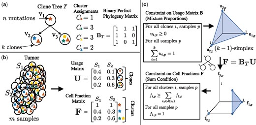
Tree constraint on cluster cell fractions. (a) We model the evolution of a tumor as a clone tree T, with k vertices corresponding to clones in the tumor. A mutation (denoted here by a star) is assigned to the clone in which it originates. Under the infinite sites assumption, a mutation occurs once, and is never lost. Thus, if a mutation occurs in clone vi, all descendent clones of vi will also contain that mutation. A clone tree T can be described by a binary perfect phylogeny matrix BT. (b) We measure m samples from a heterogeneous tumor, each sample containing a mixture of clones. The usage matrix U describes the proportion of each clone in each sample. The cell fraction matrix F describes the proportion of cells that contain a given cluster of mutations. For example, here the clone v1, containing the red mutation, occurs in of sample S1, but has a cell fraction of , as the red mutation is present in all cells. (c) As the usage matrix U describes mixture proportions, the columns of U are constrained to be on the -simplex. For a tree T, F and U are related by F = BTU. Thus, the set of allowed cell fractions for a tree T is a linear transformation of the -simplex and is unique for every distinct tree T. This set can be described by the Sum Condition, where denotes the set of children of vi in T
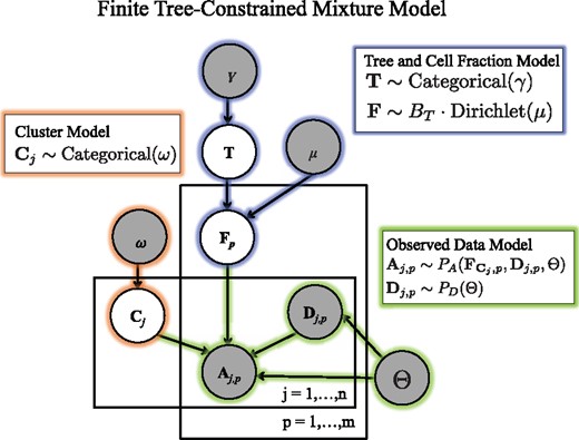
Generative model for variant allele counts A from DNA sequencing data of a tumor. A latent (unobserved) clone tree T generates m samples, each consisting of mixtures of cells with different mutations. Each mutation is assigned to a cluster . A cluster i of mutations occur in fraction of cells in sample p. Variant read counts A are generated for each mutation with a binomial likelihood model, given an observed total read counts D
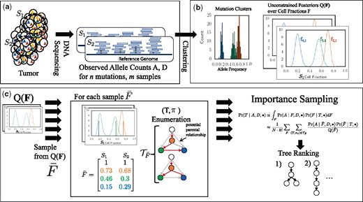
Overview of PASTRI algorithm. (a) We observe variant-allele read counts A and the total number of reads D that align to the locus for n mutations across m samples of the tumor. (b) A clustering algorithm that does not require that the data is generated by a phylogenetic tree gives an estimate of the posterior distribution over cluster cell fractions F. (c) PASTRI draws samples from . For each sample , PASTRI enumerates the set of trees T and assignments π of cell fractions to vertices of of T that satisfy the Sum Condition. All trees/vertex-assignment pairs not in have a probability of 0. Algorithm estimates the posterior probability of each tree using importance sampling
2.1 Model
We model tumor evolution using SNVs as phylogenetic characters, leaving extension to other types of genomic aberrations (e.g. copy-number aberrations) as future work. Following previous work (Deshwar et al., 2015; El-Kebir et al., 2015; Hajirasouliha et al., 2014; Jiang et al., 2016; Jiao et al., 2014; Malikic et al., 2015; Popic et al., 2015; Strino et al., 2013), we assume that each locus mutates at most once during the lifetime of the tumor, an assumption known as the infinite-sites assumption (ISA). As such, we encode the state of a locus in a cell as a binary character, with a 0 indicating the germline state and a 1 indicating a somatic mutation. We model cancer evolution as a clone tree, a directed tree with vertices (Fig. 1a). Vertex vi corresponds to a clone i in the tumor, and a directed edge (vi, vj) encodes the evolutionary relationship that clone j is a direct descendant of clone i. Equivalently, we can represent a tree T as a k × k perfect-phylogeny matrix (Gusfield, 1991). Column i of matrix BT corresponds to the genome of vertex vi, such that bij = 1 if vertex vj is on the unique path from vi to the root, and 0 otherwise.
We use cluster to refer to the set of mutations that first occur in a particular clone. We define the cluster assignment vector to be the vector mapping each mutation j to a clone v, such that cj = v indicates that v is the first clone in which mutation j occurs. By the ISA, the genomes of all descendant clones of vi also contain mutation j. The genome of a clone vi is then defined by the set of mutations assigned to vertices on the path from the root of the tree to vi.
Equivalently, (as described in El-Kebir et al. (2015)), the cell fraction matrix F is related to the tree T and usage matrix U according to F = BTU, where BT is the square binary perfect phylogeny matrix corresponding to T. As BT is invertible, we have that . Allowed cell fractions F for a tree T are then those for which is a valid usage matrix, i.e. the entries are non-negative and the columns are on the -simplex. Figure 1c shows that this constraint on the usage matrix U corresponds to the Sum Condition, and the additional constraint that the cell fraction in all samples p for germline variants in normal cells. As described in El-Kebir et al. (2015), these constraints provide a necessary and sufficient condition for a valid usage matrix (Fig. 1c).
For each mutation j identified in sample p, we measure the number of variant reads—reads that contain the somatic mutation—and the total number of reads that align to the locus. Suppose we observe data for n mutations across all samples. Let A and D be n × m matrices corresponding to the observed number of variant and total reads for each mutation. The variant-allele frequency of a mutation j in sample p is proportional to the fraction of cells containing the variant in the mixture. Under the infinite sites assumption with a diploid genome, this fraction is , as each cell containing the mutation has one mutated and one unmutated copy.
2.2 Probabilistic model
We model the observed data using a finite tree-constrained mixture model (Fig. 2). We divide the model into three components: the tree and cell fraction model (highlighted in blue), the cluster assignment model (orange), and the observed data model (green).
We first describe the tree and cell fraction model. Let T be the random variable corresponding to the latent unobserved clone tree. We assume that T follows a categorical distribution which selects tree T with weight γT. For the results in this paper, we set γ such that the probability of all trees is uniform. As the columns of a usage matrix lie on the -simplex, i.e. all entries are non-negative and for all samples p, we model the usages for sample p using a Dirichlet distribution, with vector of hyperparameters μ of length k.
Under this model, any matrix U whose columns are not on the -simplex will have a probability . This implies that the cell fractions for sample p are distributed as , where BT is the perfect phylogeny matrix corresponding to tree T. As described in Section 2.1, for a valid usage matrix U, respects the Sum Condition for tree T. Thus, a cell fraction matrix F will have non-zero probability if and only if it respects the Sum Condition across all samples.
As in a standard mixture model, the observed data is composed of mixtures of k clusters. Let be the random variable corresponding to cluster assignments where follows a categorical distribution parameterized by weights ω. Under this model, the cluster assignments are conditionally independent given the fixed hyperparameter ω. This choice allows us to easily marginalize over possible cluster assignments during inference, described below. Note that this model differs from a Dirichlet process mixture models, where the number of clusters is not fixed, and the cluster assignments have a complex dependence on each other.
Let A and D be the random variables corresponding to the number of variant and total reads across n mutations and p samples. Under the infinite sites assumption, we expect the variant-allele frequency of a mutation j in sample p to be proportional to the cell fraction of the cluster containing the mutation. That is in a diploid genome. We will use a binomial model for allele counts in the present work, so that . However, the model described above allows for more sophisticated models of read counts that involve additional parameters Θ that can model sequencing error, over-dispersion, copy-number aberrations, or other features. One example of such a model, which includes probabilities of false positive and false negative mutations, is used in Section 3.2, and described in Supplementary Section SB.3. A key feature of these models is that the observed variant allele counts do not depend directly on the tree T, only on the cell fractions F. This allows us to sample cell fractions and compute the data likelihood and model parameter likelihoods separately.
2.3 Tree inference
2.3.1 Importance sampling
We now describe how we compute the integral over cell fractions F in Equation 6. Integrating, or marginalizing, over cell fractions is more complicated that marginalizing over cluster assignments as F is continuous, high-dimensional, and the entries of matrix F are not independent. Thus, we cannot analytically calculate this integral. In this section, we describe how to calculate this integral using importance sampling (Tokdar and Kass, 2010), using input from a clustering approach without a tree constraint, and a combinatorial tree enumeration algorithm. Figure 3 shows an overview the PASTRI algorithm.
In our case, the distribution of interest is . We use a clustering method, such as SciClone (Miller et al., 2014) or PyClone (Roth et al., 2014), which gives an estimate of the posterior probability over F, without the tree constraint, where we use to denote the probability under the model used by the clustering method and where indicates the distribution may depend on a number of hyperparameters. Thus, and differ primarily in the generative model for cell fractions: a tree constraint, versus no constraint . As there is an underlying tree T that generated the data, the true F respects a tree constraint on cell fractions, and thus, we expect a significant portion of posterior probability mass respects the tree constraint for T. Thus, using unconstrained is an effective approximation of constrained .
When sampling from the unconstrained posterior , cell fractions do not yet correspond to vertices of the tree. A permutation π of the rows of a sampled cell fraction corresponds to assignments of cell fractions to vertices of the tree. We denote by the permutation of the rows of . All permutations result in the same data likelihood . However, not all permutations satisfy the Sum Condition (Fig. 4). For example, consider a linear tree T, as in Figure 4. There is a single permutation that satisfies the Sum Condition: the frequencies must be in descending order. In general, for a tree on k vertices, a relatively small fraction of the total permutations will satisfy the Sum Condition. Since, cell fractions that do not respect the Sum Condition for a tree T have probability , most of the permutations of a sampled cell fraction will have a probability of 0.
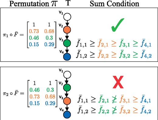
Importance sampling. The data likelihood is the same for all permutations π of for this tree T. However, satisfies the Sum Condition, and does not. Thus has a probability
Using insights from combinatorial approaches (as described in Section 2.1), we can enumerate exactly the set of trees T and permutations π for which satisfy the Sum Condition. Indeed, given cell fractions , the problem of finding a tree T and an assignment π of cell fractions to vertices of T satisfying the Sum Condition is the problem investigated in several previous works (El-Kebir et al., 2015, 2016; Malikic et al., 2015; Popic et al., 2015). El-Kebir et al. (2015) and Popic et al. (2015) describe the solutions to this problem as finding a constrained set of spanning trees of a particular graph. Popic et al. (2015) and El-Kebir et al. (2016) use a specialized version of the Gabow-Myers algorithm (Gabow and Myers, 1978) to enumerate this specific set of trees.
Note that any pair will have a probability . Thus, summing over just (Equation 10) is equivalent to summing over all permutations (Equation 9). In practice, instead of calculating the likelihood for each tree T separately, we use the same set of samples for all trees. Thus, for each sample , we only need to enumerate once.
3 Results
3.1 Benchmarking on simulated data
We compare PASTRI to three other methods for constructing tumor phylogenies: PhyloSub (Jiao et al., 2014), Canopy (Jiang et al., 2016) and AncesTree (El-Kebir et al., 2015). PhyloSub and Canopy both employ a Bayesian non-parametric model to simultaneously infer the number of clones, the most likely clusters and cluster cell fractions, and the phylogeny. AncesTree is a combinatorial method which takes as input clusters of SNVs and infers the largest tree with these clusters. We used SciClone (Miller et al., 2014) to generate clusters as input for both PASTRI and AncesTree.
We generate 50 instances each of 3, 4 and 5 vertex trees with 20 SNVs. All simulated instances contain 5 sequenced samples, each with 200X coverage. PhyloSub and Canopy were both run using default parameters. PASTRI was run for 10, 000 iterations, with uniform priors over U, C and T. We compare the methods using three metrics: accuracy in recovering ancestral relationships, accuracy in cluster cell fractions, and runtime. Further details of the simulations are in Supplementary Section SB.1.
3.1.1 Recovering the phylogenetic tree
To assess the ability of each method to recover the true phylogenetic tree, we measured the proportion of ancestral relationships between SNVs that were correctly reported in the best reported tree by each method. A pair of SNVs c and d can have one of four relationships in a tree: c and d may be in the same cluster, c may be ancestral to d, d may be ancestral to c, or c and d may be on distinct branches of the tree. For all pairs of distinct SNVs in each sample, we measure whether the reported relationship matched the relationship in the true tree. The results for 5 vertex trees are shown in Figure 5a, with results for 3 and 4 vertex trees in Supplementary Figure S3. We see that PASTRI outperforms the other three methods. On 5 vertex trees, PASTRI correctly infers all ancestral relationships on 46% of instances, while neither PhyloSub nor Canopy have a single instance on which this happens.
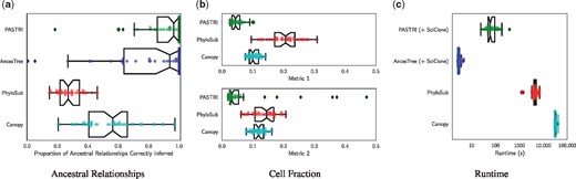
Comparison of phylogenetic reconstruction algorithms. We simulate 50 trees with 5 vertices, 5 samples and 20 mutations. (a) To quantify the accuracy of the tree inference, we measure the proportion of ancestral relationships that the algorithms correctly recover. A pair of mutations c and d has four possible ancestral relationships: c is ancestral to d, d is ancestral to c, c and d are in the same cluster, or c and d are on separate branches. (b) To measure how accurately the algorithms recover the true cell fractions, we report two metrics, given by Equations 13 and 14. Both metrics measure the average distance between the true cluster cell fraction matrix F and the reported cluster cell fractions. Metric 1 penalizes for overestimating the number of clusters, and Metric 2 penalizes for underestimating. (c) We report the runtime in seconds of each method, where the x-axis is a logarithmic scale
3.1.2 Recovering cluster cell fractions
To assess each method’s ability to recover true cluster cell fractions, we compare the true cluster cell fractions F to the reported cluster cell fractions and , for PASTRI, PhyloSub and Canopy respectively. We do not compare to AncesTree in this section since we used SciClone clusters and cell fractions as input to AncesTree. Since an algorithm may return a different number of clusters than the true number of clones, we use two different metrics to measure accuracy Let be the average per-entry distance between two rows. Let be the inferred number of clusters.
- Metric 1 – A measure of sensitivity, matches the true clones to the nearest reported clusters.(13)
- Metric 2 – A measure of specificity, matches the reported clusters to the nearest true clones.(14)
3.1.3 Runtime
We compare the runtime of the four algorithms, using the combined runtime of SciClone clustering and tree inference for PASTRI and AncesTree. Figure 5c shows the results for 5 vertex trees. Note that these results are shown on a log scale. Supplementary Figure S2 shows the results for 3 and 4 vertex trees. Note that both PhyloSub and Canopy are sampling methods and the runtime is determined by how many samples each method uses within their default parameters. As such, we expect increasing the number of samples improves the accuracy of the methods. However, we see that PASTRI achieves higher accuracy with significantly lower runtimes than either PhyloSub or Canopy. Overall, runtimes ranged from on the order of seconds for SciClone and AncesTree, minutes for PASTRI, and hours for PhyloSub and Canopy.
3.1.4 Comparison to AncesTree
AncesTree and PASTRI rely on the same combinatorial structure for tree inference, and differ primarily in the way they handle uncertainty in variant allele frequencies. In particular, PASTRI uses a probabilistic model for observed read counts, while AncesTree relies on confidence intervals for cell fractions. Because of these similarities, we performed additional comparisons to illustrate the differences between these approaches. Since PASTRI uses a more sophisticated error model, we expect that it would perform as good as or better than AncesTree in recovering the true tree.
We generated trees with varying number of vertices (6–10), samples (2–10) and coverage (50X–500X). For these experiments, we generated 50 trees, and the parameters that were not being varied were fixed to k = 5 vertices, m = 5 samples, and coverage . Each tree contained n = 50 mutations. Here we report the proportion of ancestral relationships correctly inferred by AncesTree and by the maximum likelihood tree found by PASTRI.
Figure 6a shows that as coverage increases, the performance of both methods improves. Overall, PASTRI outperforms AncesTree across all coverages, but we see the largest effect at high coverage. At low coverage, there is considerable uncertainty in variant allele frequencies, and thus, many trees are indistinguishable by likelihood. While AncesTree reports a single tree, PASTRI provides a posterior over all trees, reflecting the level of uncertainty in the reconstruction. As the coverage increases, PASTRI sees larger gains in performance. Interestingly AncesTree performance declines in the highest coverage. This effect may be due to the error model for AncesTree. As the coverage increases, confidence intervals over cluster cell fractions become narrower. Thus small errors in the initial clustering by SciClone may result in violations of the Sum Condition (described in Section 2.1 and Fig. 1).
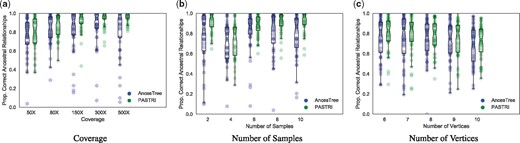
The effect of coverage, number of samples, and number of vertices on performance of AncesTree and PASTRI. For every combination of parameters, we generate 50 trees. Here we report the proportion of ancestral relationships that were correctly recovered. Overall, PASTRI has higher average performance for all sets of parameters, but the magnitude of this effect differs. (a) As the coverage increases, and uncertainty in variant allele frequencies decreases, PASTRI’s accuracy increases. AncesTree’s accuracy increases initially, but declines at the highest coverages. (b) Similarly, as the number of samples increases and the problem becomes more constrained, PASTRI’s accuracy increases, while AncesTree’s accuracy peaks with four samples, and then declines. (c) As the number of vertices in the tree increase, both AncesTree and PASTRI see a similar moderate decline in performance, although PASTRI consistently outperforms AncesTree
As the number of samples increases, the Sum Condition becomes a stronger constraint. Thus, we expect a corresponding increase in accuracy. Figure 6b shows that this is indeed the case for PASTRI. However, for AncesTree, we see that after 4 samples, performance begins to decline. This too is likely attributed to the simpler model of uncertainty in cell fractions employed by AncesTree. For a cluster, if the Sum Condition is violated in any sample, then that cluster is not included in the tree. Thus, increasing the number of samples results in a decline in performance for AncesTree.
To evaluate the performance of AncesTree and PASTRI on different size trees, we used parameters r = 100 and m = 5 where the two algorithms showed similar performance for smaller trees. We see a moderate decline in performance of both algorithms as the number of vertices grow. This is not surprising since the number of possible trees grows exponentially with the number of vertices, but the amount of observed data A and D remains fixed. PASTRI consistently outperforms AncesTree on both average and worse case, for nearly all size trees.
3.2 Chronic lymphocytic leukemia
Rose-Zerilli et al. (2016) sequenced 13 patients with chronic lymphocytic leukemia (CLL). Each patient had 2–5 samples taken longitudinally over the course of their disease and these were subjected to a number of analyses including targeted deep sequencing. The authors classify the patients into those with linear phylogenies (4/13 patients) and those with complex branching phylogenies (9/13 patients) on the basis of PhyloSub (Jiao et al., 2014) analysis. Branching phylogenies are used as evidence of subclonal competition prior to therapy.
Here we investigate Patient 5 in the study. This patient was classified as having a complex branching phylogeny (Fig. 7) using PhyloSub analysis. For this patient, SciClone inferred 8 clusters of mutations. Running PASTRI results in an optimal tree with 8 vertices that is mostly linear. The fully linear tree was ranked third out of 115 trees. We calculate the likelihood of the data under both the PASTRI read count observation model, and the PhyloSub read count model, which allows for sequencing error (i.e. false positives and negatives) in observations. Details on these models can be found in Supplementary Section SB.3. Under both models, the likelihood for both trees found by PASTRI are higher than the branching phylogeny reported in Rose-Zerilli et al. (2016). There are two possible explanations for the discrepancy. First, it is possible that PhyloSub’s sampling procedure never found either the optimal tree or the linear tree. Second, the tree-structured stick breaking prior over trees used by PhyloSub has hyperparameters that influence the width and the depth of the trees. As a result, the branching phylogeny presented may have been preferred to a linear phylogeny. However, if an intention of a study is to classify patients by phylogenetic tree structure, it makes sense to use non-informative priors over trees.
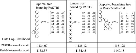
Patient 5 from Rose-Zerilli et al. (2016). This patient was classified as having a complex branching phylogeny using PhyloSub analysis (right). Running PASTRI finds an optimal phylogeny that is mostly linear (left). Restricting to linear phylogenies results in the center tree, which was the third most likely phylogeny out of 115 possible. We calculate the likelihood of the data under both the PASTRI read count observation model, and the PhyloSub observation model that also models sequencing error in observations. Under both models, the likelihood for both trees found by PASTRI are better than the reported branching phylogeny
We analyzed this same patient using AncesTree. AncesTree was not able to find a tree relating all 8 clusters. Supplementary Figure S6 shows the largest tree found by AncesTree, containing 6 clusters, and 18/20 mutations.
4 Discussion
We introduced PASTRI, a new method that simultaneously clusters mutations and infers tumor phylogenies from bulk-sequencing data. PASTRI exploits the conditional independence of the observed read counts from the latent phylogenetic tree given the cluster cell fractions. Because of this conditional independence, we are able to exploit combinatorial constraints (El-Kebir et al., 2015; Jiao et al., 2014; Malikic et al., 2015; Popic et al., 2015; Strino et al., 2013) to efficiently marginalize over cluster cell fractions, using a combinatorial tree enumeration algorithm. At the same time, we utilize a probabilistic model for the observed read counts that models errors and uncertainty in sequencing data. By leveraging combinatorial structure into the probabilistic inference, we obtain improved accuracy over prior combinatorial algorithms—due to better modeling of uncertainty in the sequence data—and improved runtime over probabilistic methods—due to more efficient inference.
By using importance sampling, we direct the computation toward regions of the sample space with highest probability. As a result, PASTRI will calculate more precisely the posterior probability of the trees that have the higher probability versus trees that have low probability. In our application, this is an acceptable tradeoff, as we are most interested in recovering the highest probability trees, and generally are not concerned with ranking highly unlikely trees. Note that our importance sampling approach can use any algorithm that computes a posterior distribution over clusters; we have used SciClone (Miller et al., 2014) in this work, but PyClone (Roth et al., 2014), Clomial (Zare et al., 2014) or other algorithms can also be used.
In Section 3.2, we examined data from a study that aimed to classify patients as having either a linear of a complex branching phylogeny. We showed a case where an existing algorithm failed to find a linear phylogeny that had higher likelihood than the reported branching phylogeny. In cases with few samples or low coverage, there is significant ambiguity in the tree structure, and many trees may have similar likelihood. Reporting the single solution of highest likelihood may not accurately recover the underlying phylogeny. In particular, when distinguishing between linear and branching phylogenies, there may be many branching trees, but only a single linear tree. Thus, it is important to consider the posterior distribution over tree topologies, particularly when correlating topology to other clinical features.
There are a number of directions for future work. First is to improve the model selection problem of choosing the number of clones/clusters. In this work, we relied on the model selection procedure performed by the clustering algorithm. However, it is plausible that in some scenarios the phylogenetic tree constraint would shift cluster cell fractions in such a way to affect the choice of the number of clones. Second, while we have demonstrated PASTRI using single-nucleotide mutations, the hybrid combinatorial-probabilistic approach generalizes to the analysis of copy-number aberrations (CNAs), which are widespread in solid tumors. As CNAs affect the observed allele counts of single-nucleotide mutations in a predictable way (as described in Deshwar et al. 2015; El-Kebir et al. 2016), the interaction between observed CNAs and allele counts can be modeled. Finally, the hybrid inference algorithm presented here could generalize to other problems where there is conditional independence between a combinatorial structure (here a tree) and a probabilistic model.
Funding
This work is supported by a US National Science Foundation (NSF) CAREER Award (CCF-1053753) and US National Institutes of Health (NIH) grants R01HG005690, R01HG007069, and R01CA180776 to BJR. BJR is supported by a Career Award at the Scientific Interface from the Burroughs Wellcome Fund, an Alfred P. Sloan Research Fellowship.
Conflict of Interest: B. Raphael is a founder and consultant of Medley Genomics.
References

