


Abstract
Neocortical circuits share anatomical and physiological similarities among different species and cortical areas. Because of this, a ‘canonical’ cortical microcircuit could form the functional unit of the neocortex and perform the same basic computation on different types of inputs. However, variations in pyramidal cell structure between different primate cortical areas exist, indicating that different cortical areas could be built out of different neuronal cell types. In the present study, we have investigated the dendritic architecture of 90 layer II/III pyramidal neurons located in different cortical regions along a rostrocaudal axis in the mouse neocortex, using, for the first time, a blind multidimensional analysis of over 150 morphological variables, rather than evaluating along single morphological parameters. These cortical regions included the secondary motor cortex (M2), the secondary somatosensory cortex (S2), and the lateral secondary visual cortex and association temporal cortex (V2L/TeA). Confirming earlier primate studies, we find that basal dendritic morphologies are characteristically different between different cortical regions. In addition, we demonstrate that these differences are not related to the physical location of the neuron and cannot be easily explained assuming rostrocaudal gradients within the cortex. Our data suggest that each cortical region is built with specific neuronal components.
Introduction
The search for guiding principles to understand the function of the cortical circuit has a long history. Cajal devoted many pages to speculations on potential functions that could be implemented by the anatomical pattern of neuronal morphologies and axonal innervation observed (Ramón y Cajal, 1899). His disciple Lorente de Nó described more than a hundred types of cortical neurons in mouse temporal cortex (Lorente de Nó, 1922) and characterized cortical circuits as vertical chains of neurons (Lorente de Nó, 1949). Based on electrophysiological recordings, Mountcastle, and later Hubel and Wiesel, proposed the columnar hypothesis, by which the neocortex would be composed of repetitions of one basic modular unit, and argued that the same basic cortical computation could be performed by a cortical module in different cortical areas (Hubel and Wiesel, 1974, 1977; Mountcastle, 1982, 1997). Thus, the task of understanding cortical function could be reduced to deciphering the basic ‘transfer function’ that that module performs on any input. The differences in function among different cortical areas would then be explained by the difference in the inputs they receive, rather than by intrinsic differences on cortical processing among areas.
In more recent times, Douglas and Martin have termed this idea the ‘canonical microcircuit’ hypothesis and have proposed a series of basic circuit diagrams based on anatomical and electrophysiological data (Douglas et al., 1989, 1995; Douglas and Martin, 1991, 1998, 2004). According to their hypothesis, the common transfer function that the neocortex performs on inputs could be related to the amplification of the signal (Douglas et al., 1989) or a ‘soft’ winner-take-all algorithm (Douglas and Martin, 2004). These ideas agree with the recurrent excitation present in cortical tissue which could then exert a top-down amplification and selection on thalamic inputs (Douglas et al., 1995).
There are many arguments in favor of a canonical microcircuit. Besides the electrophysiological evidence based on receptive fields, the anatomical presence of vertical chains of neurons defining small columnar structures has been noted since Lorente (Lorente de Nó, 1949). According to him, myelin stains show vertical bundles of pyramidal cell axons. Similar bundles of apical dendrites have been noticed by a number of authors using a variety of staining methods (Fleischauer, 1972; Fleischauer and Detze, 1975; Escobar et al., 1988; Peters and Yilmaz, 1993; Peters and Walsh, 1972). These structural modules appear in many different regions of the cortex in many different species (e.g. Buxhoeveden et al., 2002). In addition, support for the idea of canonical microcircuits has come from the basic stereotyped developmental program that different cortical regions (and cortices from different species) share (Purves and Lichtman, 1985; Jacobson, 1991). Like in other parts of the body, it is possible that the neocortex arose by a manifold duplication of a similar circuit module. The relatively short evolutionary history of the neocortex, together with the prodigious increase in size it has experienced in mammals, makes this idea appealing. Also, all cortices of all animals develop through a very stereotypical sequence of events, from neurogenesis in the ventricular zone, to migration along radial glia, depositing of neuroblasts in cortical layers and emergence of axons, dendrites and dendritic spines. These events occur in some cases with nearly identical timing in different parts of the cortex and in different animals, so it is not unreasonable to argue that they result in the assembly of an essentially identical circuit. Nevertheless, important differences in the specification of cortical areas have also been noted (Rakic, 1988). Finally, it is still unclear how much of the connectivity matrix is determined by early developmental events, and how much could be locally regulated or even controlled by activity-dependent Hebbian rules (Katz and Shatz, 1996). In this respect, transplantation experiments have indicated that axons from the visual pathway, when rerouted to the auditory or somatosensory areas, generate in the host neurons receptive properties which are similar to those found in visual cortex (reviewed in Sur, 1993; Frost, 1999). These data could be interpreted as supportive of the idea of canonical microcircuits, but could also be explained as the product of developmental plasticity mediated by novel axons or axonal activity. A final argument in support for a canonical microcircuit comes from the stereotypical laminar and columnar input–output organization of the cerebral cortex (Gilbert and Wiesel, 1979; Jones, 1981).
On the other hand, there are also compelling reasons against this hypothesis. It is hard to imagine that there is a common denominator in all the different computational problems that the cortex is solving. In some cases, these problems appear mathematically irreducible even in their basic dimensionality, such as three-dimensional visual processing, as compared with auditory speech perception, for example. Also, the exact nature of the structure of the cortical modules is hard to define. Anatomical techniques do not reveal any clear borders between modules, and physiological approaches show instead, like in the primate primary visual cortex, a combination of maps superimposed onto one another with different metrics, such as orientation, ocular dominance, or spatial frequency (Bartfeld and Grinvald, 1992), although perhaps a more basic metric could underlie them (Basole et al., 2003).
Furthermore, if evolution was duplicating circuit modules in different cortical areas or in the cortex of different animals, it would be expected that a canonical microcircuit, in the strict sense, would be built with the same components. Thus, the neuronal cell types and connections between these neurons should be very similar or even identical. In this respect, although it is generally agreed that cortical areas have the same complement of neuronal cell types (e.g. Rockel et al., 1980), in some cases there are distinct types of neurons which are only found in particular cortical areas or species, such as the Meynert and the Betz giant pyramidal neurons, or certain types of spindle neurons and double bouquet cells (Nimchinsky et al., 1999; DeFelipe et al., 2002; Ballesteros-Yáñez et al., 2005). In addition, recent work has demonstrated that the most typical and abundant neuron in cortex, the pyramidal cell, sampled from different areas of different primate species, has quantitative differences in the size of the dendritic arbor and in the density of spines (Elston et al., 1997, 2001, 2005a; Elston and Rosa, 1997; Benavides-Piccione et al., 2002; DeFelipe et al., 2002; Elston and DeFelipe, 2002). However, it remains unknown whether this is a general evolutionary trend, or if in small-brained species, e.g. mice, circuits in different cortical areas have similar cellular components. Furthermore, from previous studies it is difficult to determine if these cortical differences represent a systematic gradient of morphological features, as occurs in other parts of the body plan. Also, available data only take into account measurements of individual morphological parameters to evaluate how different or similar two neuronal morphologies are based on measurements of individual morphological parameters. What constitutes two different neuron types to one investigator could become a single group to another.
To rigorously address these questions, in the present study we investigated the basal dendritic arbors of layer II/III pyramidal neurons from three different and distant regions of the mouse neocortex: the secondary motor cortex (M2), the secondary somatosensory cortex (S2), and the lateral secondary visual cortex and association temporal cortex (V2L/TeA), using principal component analysis (PCA)-based cluster analysis of the multidimensional dataset of 156 morphological parameters sampled from three-dimensional reconstructions. To avoid methodological problems, we used an unbiased sampling method and the same technical conditions for all neurons. We chose to study the basal dendritic arbors in horizontal sections to systematically compare a complete and major dendritic region of the pyramidal neurons, and because the majority of quantitative studies of pyramidal cell structure in the cerebral cortex have been performed on the basal dendritic arbors of layer III in different primate species and cortical areas. We also sampled neurons from the same animals to prevent differences between animals. Using cluster analysis we determined the statistical properties of the neurons in each of the three cortical areas chosen and directly plotted their differences in variance, while keeping track of the exact position of each neuron in the cortex. Our data confirm the existence of systematic morphological differences among neurons of different cortical regions. Moreover, we find that the key difference lies in the size of their dendritic trees. Finally, we cannot account for these differences assuming a simple gradient of sizes across the cortex. The simplest interpretation of our data is that each cortical region is built with different types of pyramidal neurons.
Materials and Methods
Tissue Preparation and Intracellular Injections
BC57 Black mice (n = 2, 2 months old) were overdosed by intraperitioneal injection of sodium pentobarbitone and perfused intracardially with 4% paraformaldehyde. Their brains were then removed and the cortex of the right hemisphere flattened between two glass slides (e.g. Welker and Woolsey, 1974) and further immersed in 4% paraformaldehyde for 24 h. Sections (150 μm) were cut parallel to the cortical surface with a Vibratome. By relating these sections to coronal sections we were able to identify, by cytoarchitectural differences, the section that contained layer II/III among the rest of cortical layers allowing the subsequent injection of cells at the base of layer II/III (e.g. see Fig. 3 of Elston and Rosa, 1997). Our cell injection methodology has been described in detail elsewhere (Elston et al., 1997, 2001; Elston and DeFelipe, 2002). Briefly, cells were individually injected with Lucifer Yellow in three different regions of the neocortex [approximately corresponding to areas M2, S2 and V2L/TeA of Franklin and Paxinos (1997)] by continuous current that was applied until the distal tips of each dendrite fluoresced brightly. Following injections, the sections were processed with an antibody to Lucifer Yellow, as described in Elston et al. (2001) to visualize the complete morphology of the cells (Fig. 1). Only neurons that had an unambiguous apical dendrite and whose basal dendritic tree was completely filled and contained within the section were included in this analysis.
![Reconstruction of mouse layer II/III pyramidal cells' basal dendrites. (A) Low-power photomicrograph of the mouse cerebral cortex cut parallel to the cortical surface, showing the regions where cells were injected [approximately corresponding to areas M2, S2 and V2L/TeA of Franklin and Paxinos (1997) respectively]. These neurons were injected in layer II/III with Lucifer Yellow and then processed with a light-stable diaminobenzidine. (B–J) Successive higher magnification photomicrographs showing pyramidal cells basal dendrites in M2 (B, E, H), S2 (C, F, I) and V2L/TeA (D, G, J) regions. Scale bar = 815 μm in A; 350 μm in B–D; 150 μm in E–G; 60 μm in H–J.](https://oup.silverchair-cdn.com/oup/backfile/Content_public/Journal/cercor/16/7/10.1093_cercor_bhj041/2/m_cercorbhj041f01_ht.jpeg?Expires=1716475456&Signature=gbgm4KHdjsaVlFlsZOwwYnrz1bMzC5U4q2QIwuCmDVwiN8cSOt12HuFEBxB825LP8j9act3OJmFsTOU0crg9pjQTj-QnOcf1W-bZpbycUirULVeiKd~u0RDy-dnxasN3mK-U4bKfoJz8tbLO6TxZ2GkHjfKO45UXYrsPWC-0CIXNjMh0cJ7Jol9ixcIRBfYPYGEK0zxNRtZVCBDp~qcrH9WvSUiaD225-0FnuBcGHL1Kp84vNhMyEiz1vPYFzWRQ76Um1ALh7lubrIsy1AENSz3OmYiTWrfD4hQh2ufjFRYmxNu5NwNUP6NlfpHhJ-PspDH3rT23Xgi3Hci5q8-lYA__&Key-Pair-Id=APKAIE5G5CRDK6RD3PGA)
Reconstruction of mouse layer II/III pyramidal cells' basal dendrites. (A) Low-power photomicrograph of the mouse cerebral cortex cut parallel to the cortical surface, showing the regions where cells were injected [approximately corresponding to areas M2, S2 and V2L/TeA of Franklin and Paxinos (1997) respectively]. These neurons were injected in layer II/III with Lucifer Yellow and then processed with a light-stable diaminobenzidine. (B–J) Successive higher magnification photomicrographs showing pyramidal cells basal dendrites in M2 (B, E, H), S2 (C, F, I) and V2L/TeA (D, G, J) regions. Scale bar = 815 μm in A; 350 μm in B–D; 150 μm in E–G; 60 μm in H–J.
Reconstruction of Cortical Neurons
The Neurolucida package (MicroBrightField) was used to three-dimensionally trace the basal dendritic arbor of pyramidal cells in each cortical region. All neurons that were judged to be completely filled (as evident by the termination of all their dendritic branches in a normally round tip, far from the plane of section and without any graded loss of stain) were included for analysis. For each reconstructed basal skirt (30 in M2, 30 in S2, 30 in V2L/TeA), we performed the branched structure, convex hull, Sholl, fractal, fan in diagram, vertex, and branch angle analyses (incorporated in the Neurolucida package) and measured a battery of 156 morphological parameters that included features of the basal dendritic tree and the soma (Supplementary Table 1):We thus generated a database of all these parameters to characterize each of the 90 cells and analyzed this data matrix for the rest of the study.
Total number of nodes (branch points) and endings (end or termination points) contained in the basal dendritic arbor.
Total dendritic length (per cell) and mean length (taking into account the quantity of dendrites) of basal dendritic arbor.
Basal dendritic field area (BDFA), which measures the area of the dendritic field of a neuron calculated as the area enclosed by a polygon that joins the most distal points of dendritic processes (convex area).
Somatic aspects, such as length (perimeter), surface area, minimum and maximum feret (which gives information about the shape, and refers to the smallest and largest dimensions of the soma contour as if a caliper had been used to measure across the contour), compactness (which describes the relationship between the area and the maximum diameter, being the compactness for a circle = 1), convexity (which measures one of the profiles of complexity, being the convexity of circles, ellipses and squares = 1), form factor (which refers to the shape of the contour, being 1 a perfect circle and approaching 0 as the contour shape flattens out; this variable differs from the compactness by considering the complexity of the perimeter of the object), roundness (i.e. the square of the compactness), aspect ratio (which evaluates the degree of flatness as the ratio of its minimum diameter to its maximum diameter), and solidity (i.e. the area of the contour divided by the convex area).
Number of dendritic branches that intersect concentric spheres (centered on the cell body) of increasing 25 μm radii and number of nodes, endings and lengths of dendritic segments as a function of the distance from the soma in the same concentric spheres.
Number of branches, nodes, endings and length of dendrites by branch order.
The fractal analysis addresses the issue of quantities being dependent on scale, and to what degree the dendritic arbor has a scale-invariant topology. K-dim of fractal analysis is the value that describes the way in which neurons fill space.
Torsion ratio of fan in diagram, which indicates the length of the dendrites divided by the length of the dendrites after applying the fan in projection, which is necessary to analyze any preferred orientation in the dendritic processes.
Vertex analysis classifies nodes on the connectivity at the vertices (connection points for the branches) and on the connectivity of the next order of vertices. This analysis compares dendritic structures combing topological and metrical properties, such as nodes and branch lengths, respectively, to describe the overall structure of a dendritic arbor: bifurcating nodes that have 2 terminating branches attached (VA), 1 terminating branch attached (VB) and 0 terminating branches attached (VC) and the rare trifurcating nodes that have 3, 2, 1 and 0 terminating branches attached (Va′, Vb′, Vc′, Vd′, respectively). The ratio Va/Vb above 1 suggests that the tree is non-random and symmetrical; values around 1 suggests that the terminal nodes growth in a random process; values <0.5 suggest that the tree is non-random and asymmetrical. All these values are expressed by branch order and per cell.
Branch angle analysis: planar angle (which describes the change in direction from one branch to the next branch and emphasizes the overall structure of the tree), local angle (which describes the change in direction using the line segments closest to the node and, unlike the planar angle, the local angle disregards the overall structure of the tree and concentrates on the information at the nodes) and spline angle (designed to get around the problems that can affect the local angle by drawing the simplest curves that can be traced through three-dimensional space (cubic curves) and taking the change in direction in the tangents formed at the ends of the cubic curves). All branch angle values are expressed by branch order and per cell.
The tortuosity of branches, is the ratio of the actual length of the segment divided by the distance between the endings of the segment, being the smallest tortuosity possible (a straight segment) = 1. These values are expressed by branch order and per cell.
Principal Component Analysis and Cluster Analysis
We eliminated parameters that would not contribute any information to our analysis. This was done in two steps: we first eliminated parameters that carried no variance across all basal skirts (consistently taking the same value in each measurement), e.g. the number of dendritic end-points at 25 μm was consistently zero for all neurons. Based on the correlation matrix of our parameters, we then eliminated parameters that showed high absolute correlation values (≥|0.8|).
To achieve a graphical representation of the distribution of basal skirts in this reduced-dimensional parameter space, we applied PCA to the correlation matrix of our parameters. The goal of this analysis was to evaluate and identify the existence of sensible clusters of basal skirts with similar features, and to identify possible outliers. The distribution of basal skirts was then plotted in the reduced two-dimensional space made of the first two principal components (PCs). It was therefore possible to visualize the distribution of basal skirts in only two dimensions and explore the existence of reasonable clusters as well as potential ‘outlying’ cases.
The central idea of PCA is to reduce the dimensionality of a data set consisting of a large number of interrelated parameters, while retaining as much as possible the variance present in the data set. This reduction is achieved by transforming original parameters to a new set of parameters, the PCs, which are uncorrelated and ordered so that the first few retain most of the variation present in all of the original parameters. Algebraically, PCs are linear combinations of original parameters. The vector of correlation coefficients (PC loadings) between each parameter and a particular PC is computed by multiplying the corresponding eigenvector of the correlation matrix by the square root of its eigenvalues. A coefficient is thus indicative of the degree of contribution of the corresponding parameter to a PC. Coefficients with absolute values equal or greater than 0.7 were considered significant and are labeled in bold (Tables 1, 2).
First two principal component loadings of neuronal basal skirt measurements. Significant correlations are in bold
| Parameters | PC 1 | PC2 |
|---|---|---|
| No. of primary branches | 0.103 | 0.298 |
| Dendritic length (μm) | −0.886 | 0.360 |
| Dendritic field surface area (μm2) | −0.598 | 0.251 |
| Somatic area (μm2) | −0.760 | 0.330 |
| Intersections at 25 μm | 0.490 | 0.747 |
| Intersections at 50 μm | −0.366 | 0.846 |
| Dendritic end-points at 50 μm | 0.382 | 0.260 |
| Dendritic end-points at 75 μm | 0.743 | 0.046 |
| Dendritic end-points at 100 μm | 0.658 | 0.256 |
| Dendritic branch-point at 75 μm | −0.816 | −0.069 |
| Dendritic branch-point at 100 μm | −0.684 | −0.404 |
| Eigenvalue | 4.370 | 1.967 |
| % Total variance | 39.729 | 17.885 |
| Cumulative % variance | 39.729 | 57.613 |
Measured parameters for V2L/TeA, S2 and M2 (outliers not included)
| V2L/TeA | S2 | M2 | |
|---|---|---|---|
| No. of primary branches | 4–9 | 3–7 | 4–8 |
| Dendritic length (μm) | 1639 ± 341a | 2140 ± 561 | 3397 ± 524 |
| Dendritic field surface area (μm2) | 22 666 ± 5130 | 31 928 ± 6358 | 61 270 ± 16 245 |
| Somatic area (μm2) | 123 ± 18 | 139 ± 22 | 179 ± 30 |
| Intersections at 25 μm | 4–20 | 8–18 | 8–17 |
| Intersections at 50 μm | 5–26 | 15–35 | 16–29 |
| Dendritic end-points at 50 μm | 0–3 | 0–2 | 0–3 |
| Dendritic end-points at 75 μm | 0–12 | 1–10 | 0–3 |
| Dendritic end-points at 100 μm | 2–13 | 4–16 | 1–9 |
| Dendritic branch-point at 75 μm | 0–6 | 0–8 | 0–9 |
| Dendritic branch-point at 100 μm | 0–6 | 0–2 | 0–6 |
Mean ± SD.
Identifying potential ‘outliers’ needs further explanation because there is no formal, widely accepted definition of an ‘outlier’. Most definitions rely on informal intuitive definitions, namely that outliers are observations that are in some way different from or inconsistent with the remainder of a data set. A major problem in detecting multivariate outliers is that an observation that is not extreme on any of the original parameters can still be an outlier, because it does not conform to the correlation structure of the remainder of the data. It is impossible to detect such outliers by looking solely at the original parameters one at a time. It is often an unusual combination of values of parameters that alienates an outlier. If the number of parameters is high, it is impossible or at least very difficult to detect such outliers since the correlation matrix would only reveal relationships of pairs of parameters.
Outliers can be of many types, which would complicate any search for directions in which outliers occur. However, there are good reasons for looking at the directions defined by either the first few or the last few PCs in order to detect outliers. The first few and last few PCs will detect different types of outliers, and in general, the last few are more likely to provide additional information that is not available in plots of the original parameters. The outliers that are detectable from a plot of the first few PCs are those that inflate variances. If an outlier is the cause of a large increase in one or more of the variances of the original parameters, then it must be extreme in terms of those parameters and thus detectable by looking at plots of single parameters.
By contrast, the last few PCs may detect outliers that are not apparent with respect to the original parameters. By examining the values of the last few PCs, we may be able to detect observations that violate the correlation structure imposed by the bulk of the data but that are not necessarily aberrant with respect to individual parameters. Therefore, a series of scatterplots of pairs of the first few and last few PCs may be useful in identifying possible outliers.
Subsequently, we used cluster analysis to objectively derive clusters of similar basal skirts. Cluster analysis was performed using Euclidian distances as the distance measure and Ward's method as the linkage rule.
Statistics
Measurements are reported as mean ± SD, except where noted. All statistical analyses were performed using STATISTICA (StatSoft, Inc., 2001; STATISTICA data analysis software system, version 6, www.statsoft.com) and the SPSS statistical package (SPSS Science, Chicago, IL).
Results
Dendritic Morphologies of Layer II/III Pyramidal Neurons
We filled layer II/III pyramidal neurons from fixed tangential slabs of the M2, S2 and V2L/TeA of the mouse neocortex with an injection of Lucifer Yellow (Fig. 1) in order to study the complete dendritic basal arbors of cells (Fig. 2). We discarded all the cells that had at least one incompletely basal dendrite, either because it was not completely filled or because it was sectioned. Our analyzed sample was 90 neurons, 30 from each of the three cortical regions. These neurons were reconstructed in three dimensions and from each neuron we measured a battery of morphological parameters that included features of the basal dendritic tree and the soma (Supplemental Table 1; see Materials and Methods for details).
Reconstructed neurons. Schematic drawings of the basal skirt of layer II/III pyramidal neurons, as seen in the plane of section parallel to the cortical surface from M2, S2 and V2L/TeA regions of the mouse cerebral cortex. Illustrated cells had basal dendritic arbors, which approximated the average size for each group. Scale bar = 100 μm.
These analyses revealed that, in general, variables showed higher values for cells in M2 than in S2, whereas the V2L/TeA region presented the lowest numbers. As can be seen from Figure 3, cells became progressively more complex in their branching structure from the caudal to rostral regions. For example, the total number of nodes, endings and length of dendrites in the whole dendritic arbor, as well as measured per distance from soma and branch order, showed significant differences between the three regions analyzed in practically all variables shown. Similarly, the basal dendritic field area, the Sholl analysis and number of branches per order in the basal arbors of these neurons showed statistically significant values between these regions (see Table 3 for detailed statistical comparisons). To further study the branching structure of neurons we also analyzed variables, such as the K-dim of fractal analysis, that describe the way in which neurons fill space, or the vertex analysis, which investigates the way in which dendritic arbors are similar or dissimilar (Fig. 4). In vertex analysis, we found that the ratio of Va/Vb, which describes the structure of the arbor, suggests that the trees are non-random and symmetrical in all three regions analyzed since values are always >1 (see Materials and Methods for details). Statistical comparisons of these variables (Table 3) revealed that, in general, cells from M2 and S2 cortical regions are more similar between each other than any other pair comparisons. In addition, some variables such as the degree of angles between dendrites or the dendritic tortuosity significantly decreased from the caudal to rostral regions.
Analysis of variables. Plot of some of the most representative variables analyzed in the present study, showing differences in the basal dendritic structure of layer II/III pyramidal cells sampled from the M2, S2 and V2L/TeA regions of the mouse cerebral cortex. Measurements are reported as mean ± SEM. Statistical significance of the differences is shown in Table 3.
Other representative variables analyzed. Measurements are reported as mean ± SEM. Statistical significance of the differences is shown in Table 3. Va, Vb and Vc represent two terminating branches attached, one terminating branch attached and zero terminating branches attached, respectively, from vertex analysis.
Principal Component Analysis of Dendritic Morphologies
To further assess this analysis, we then applied PCA to the correlation matrix to identify the parameters that carried most of the variance. After eliminating parameters that did not show significant variance across neurons or had high values of correlation with at least one of the remaining parameters, we kept 11 parameters: number of primary dendritic branches, total dendritic length, dendritic field surface area, somatic cross-sectional area, number of intersections at 25 and 50 μm, number of end-points at 50, 75 and 100 μm, and number of branch points at 75 and 100 μm (Tables 1–2).
The first two PCs accounted for 40% and 18% of the total variance respectively. For the purpose of identifying sensible clusters and outliers, the fractional variance of 58% accounted for by the first two PCs produced interpretable results. In order to detect outliers we studied distribution of basal skirts in the two-dimensional spaces made of the following PC pairs: PC1 and PC2 (Table 1); PC4 and PC5; PC5 and PC6 (data not shown). As in our previous studies (Kozloski et al., 2001; Tsiola et al., 2003), several parameters were positively correlated with each other in the first PC and could be interpreted as a measure of ‘size’ of the individual neurons, whereas subsequent PCs measured aspects of neuronal ‘topology’. Indeed, basal dendritic length, somatic area and number of dendritic branches at 75 μm showed significant correlation coefficients in PC1 (Table 1). Moreover, the coefficients all had the same sign (negative, the arbitrary signs of coefficients in PCA imply only the directions of the PC axis). In other words, these parameters were all positively correlated with each other in PC1. This means that basal skirts with larger dendritic length had more branch points at 75 μm and emanated from a larger cell body. It is not surprising to notice that larger values of the above-mentioned parameters were associated with fewer dendritic endpoints at 75 μm as implied by the significant and oppositely signed coefficient of this parameter in PC1.
The number of dendritic intersections with spheres drawn at 25 and 50 μm showed significant coefficients in PC2 (Table 1). These two parameters measured the density of the basal dendritic skirt of cortical neurons. We excluded the number of intersections at longer distances to prevent a bias toward the larger frontal basal skirts and against smaller occipital basal skirts. This also further defined the PC2 as a measurement of neuronal ‘topology’. The same sign of the coefficients for these two parameters in PC2 implied that basal skirts with more number of intersections at 25 μm tend to have more intersections at 50 μm also. The coefficient values for all other parameters were insignificant in PC2, making the task of interpreting PC2 as a measure of neuronal topology quite appropriate.
We concluded that the size of the dendritic tree and its topology could be quantitatively characterized and isolated from each other in the first two PCs.
Cluster Analysis of Dendritic Morphologies
We used the reduced dataset of 11 parameters to perform cluster analysis of the sample, using Wards' method (Fig. 5; see Materials and Methods). By considering neurons from two cortical regions at a time, we sought to maximize the discriminatory power of the cluster analysis. Indeed, in the three cluster trees, neurons from the same cortical region were overwhelmingly clustered together, with a relatively low number of outliers. Specifically, when comparing rostral and caudal regions, four (out of 30) neurons from V2L/TeA clustered with the M2 ones, whereas none of the M2 neurons clustered in the caudal group. In the M2–S2 cluster, one neuron from M2 clustered with the S2 ones, whereas only three neurons from S2 were found in the M2 cluster. Finally, in the V2L/TeA–S2 clustering, two V2L/TeA neurons clustered with the S2 group, whereas five S2 neurons clustered in the caudal group.
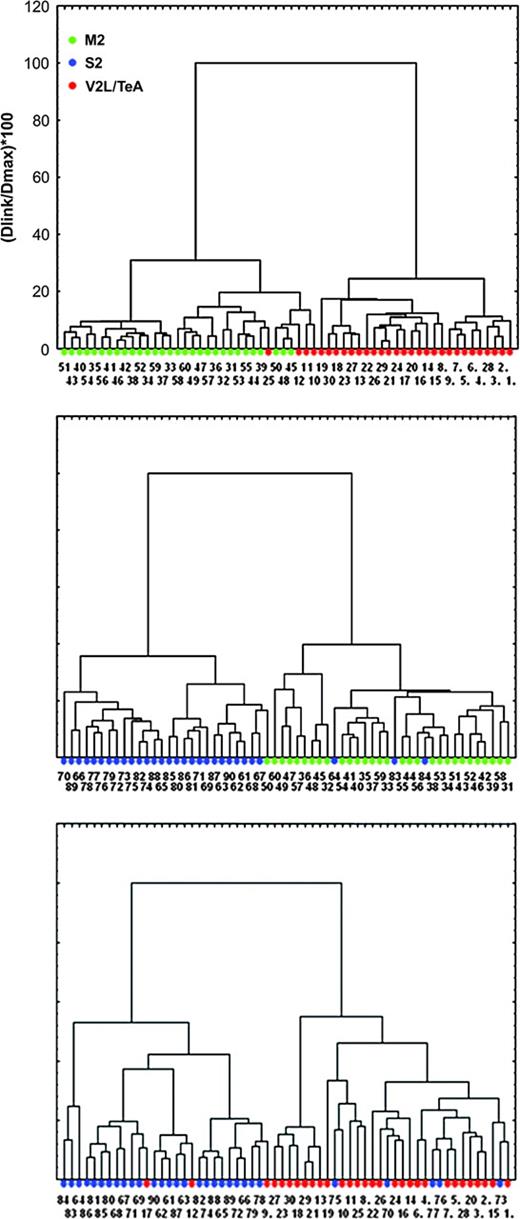
Cluster analysis. Dendrogram showing cluster analysis (Euclidean distances, Ward's method) results for all basal skirts. Basal skirts are divided into M2 (green), S2 (blue) and V2L/TeA (red) clusters. Numbers at the bottom of each tree branch denote the neuron identification number.
Our analysis thus indicated that, with the exception of some outliers (15 out of 180 possible assignments: Fig. 5, neurons 9, 10, 11, 12, 17, 25, 50, 64, 70, 73, 75, 76, 77, 83, 84), the morphologies of neurons from these three cortical regions is sufficiently distinct, so that the location of the neurons can be identified by measuring 11 morphological parameters.
Neurons from the Same Cortical Regions Are Clustered Together
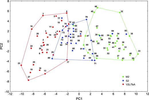
We then proceeded to study the statistical relation between the morphologies of our sampled neurons in the three cortical regions. Figure 6 shows the distribution of all the cells in the reduced two-dimensional space of the first two PCs. Superimposed on this plot are convex hulls for the clusters obtained from the cluster analysis. Convex hulls are useful in indicating areas of a two-dimensional plot covered by various subsets of observations.
Principal component analysis. Neuronal basal skirt measurements, plot of the first two PCs for 90 neurons. Clusters of neurons are well differentiated along the first principal component. Lines demarcating convex hulls reveal overlapping clusters. One neuron belonging to V2L/TeA (neuron 25), four S2 neurons (77, 83, 84, 85) and one M2 neuron (50) lie outside the boundaries of their respective clusters.
This analysis showed that the neurons covered a continuum of points along the two PC axes. At the same time, except for some outliers, most neurons from the same cortical region were located in neighboring positions. Thus, each region had a clearly defined spatial distribution and there was clear evidence of a strong cluster structure. The separation of clusters was mainly in terms of PC1 (overall size) with very little differentiation in terms of PC2. The clusters also classified the data in a sensible looking manner as was apparent from their non-convoluted shape on the PC plot.
Within the three groups of neurons, the V2L/TeA and M2 neurons were located at opposite extremes of the distribution, whereas the S2 neurons were overlapping in the center. In fact, the areas covered by caudal and rostral neurons did not overlap at all and the two clusters largely occupied different areas of the diagram. The plot, therefore, displays the interesting result that the two clusters of observations corresponding to the two cortical regions could be reproduced with utmost precision mainly in terms of their overall size. The cluster of caudal neurons had ‘size’ measurements (parameters with significant coefficients on PC1) that were all significantly different from those forming the cluster of rostral neurons (Tables 2 and 3).
| V2L/TeA-S2 | S2-M2 | M2-V2L/TeA | |
|---|---|---|---|
| Total nodes [one-way ANOVA, F(2,89) = 25.81, P < 0.001] | ** | * | ** |
| Nodes per distance from soma [repeated-measures ANOVA, F(2,87) = 25.70, P < 0.001] | ** | * | ** |
| Nodes per branch order [repeated-measures ANOVA, F(2, 87) = 26.86, P < 0.001] | ** | * | ** |
| Total endings [one-way ANOVA, F(2,89) = 31.74, P < 0.001] | ** | * | ** |
| Endings per distance from soma [repeated-measures ANOVA, F(2,87) = 9.47, P < 0.001] | ** | * | |
| Endings per branch order [repeated-measures ANOVA, F(2,87) = 34.56, P < 0.001] | ** | ** | ** |
| Total length [one-way ANOVA, F(2,89) = 96.71, P < 0.001] | ** | ** | ** |
| Length per distance from soma Repeated-measures ANOVA, F(2,87) = 91.30, P < 0.001] | ** | ** | ** |
| Length per branch order [repeated measures ANOVA, F(2,87) = 105.32, P < 0.001] | ** | ** | ** |
| Basal dendritic field area (μm2) [one-way ANOVA, F(2,89) = 107.07, P < 0.001] | ** | ** | ** |
| Sholl analysis [repeated-measures ANOVA, F(2,87) = 94.71, P < 0.001] | ** | ** | ** |
| Quantity of branches per order [repeated-measures ANOVA, F(2,87) = 31.38, P < 0.001] | ** | * | ** |
| Fractal analysis, K-dim [one-way ANOVA, F(2,89) = 18.57, P < 0.001] | ** | ** | |
| Total Va [one-way ANOVA, F(2,89) = 16.92, P < 0.001] | ** | ** | |
| Total Vb [one-way ANOVA, F(2,89) = 8.50, P < 0.001] | ** | ||
| Total Vc [one-way ANOVA, F(2,89) = 10.27, P < 0.001] | * | ** | |
| Ratio Va/Vb [one-way ANOVA, F(2,89) = 0.71, P = 0.49] | |||
| Va per order [repeated-measures ANOVA, F(2,87) = 16.92, P < 0.001] | ** | ** | |
| Vb per order [repeated-measures ANOVA, F(2,87) = 8.50, P < 0.001] | ** | ||
| Vc per order [repeated-measures ANOVA, F(2,87) = 10.27, P < 0.001] | * | ** | |
| Total planar angle [one-way ANOVA, F(2,89) = 40.72, P < 0.001] | ** | ** | |
| Total local angle [one-way ANOVA, F(2,89) = 10.55, P < 0.001] | * | ** | |
| Total spline angle [one-way ANOVA, F(2,89) = 22.42, P < 0.001] | ** | ** | |
| Total tortuosity [one-way ANOVA, F(2,89) = 10.16, P < 0.001] | ** | * | |
| Cell body area (μm2) [one-way ANOVA, F(2,89) = 40.78, P < 0.001] | * | ** | ** |
Post-hoc Bonferroni analysis, P < 0.001.
Post-hoc Bonferroni analysis, P < 0.05.
| V2L/TeA-S2 | S2-M2 | M2-V2L/TeA | |
|---|---|---|---|
| Total nodes [one-way ANOVA, F(2,89) = 25.81, P < 0.001] | ** | * | ** |
| Nodes per distance from soma [repeated-measures ANOVA, F(2,87) = 25.70, P < 0.001] | ** | * | ** |
| Nodes per branch order [repeated-measures ANOVA, F(2, 87) = 26.86, P < 0.001] | ** | * | ** |
| Total endings [one-way ANOVA, F(2,89) = 31.74, P < 0.001] | ** | * | ** |
| Endings per distance from soma [repeated-measures ANOVA, F(2,87) = 9.47, P < 0.001] | ** | * | |
| Endings per branch order [repeated-measures ANOVA, F(2,87) = 34.56, P < 0.001] | ** | ** | ** |
| Total length [one-way ANOVA, F(2,89) = 96.71, P < 0.001] | ** | ** | ** |
| Length per distance from soma Repeated-measures ANOVA, F(2,87) = 91.30, P < 0.001] | ** | ** | ** |
| Length per branch order [repeated measures ANOVA, F(2,87) = 105.32, P < 0.001] | ** | ** | ** |
| Basal dendritic field area (μm2) [one-way ANOVA, F(2,89) = 107.07, P < 0.001] | ** | ** | ** |
| Sholl analysis [repeated-measures ANOVA, F(2,87) = 94.71, P < 0.001] | ** | ** | ** |
| Quantity of branches per order [repeated-measures ANOVA, F(2,87) = 31.38, P < 0.001] | ** | * | ** |
| Fractal analysis, K-dim [one-way ANOVA, F(2,89) = 18.57, P < 0.001] | ** | ** | |
| Total Va [one-way ANOVA, F(2,89) = 16.92, P < 0.001] | ** | ** | |
| Total Vb [one-way ANOVA, F(2,89) = 8.50, P < 0.001] | ** | ||
| Total Vc [one-way ANOVA, F(2,89) = 10.27, P < 0.001] | * | ** | |
| Ratio Va/Vb [one-way ANOVA, F(2,89) = 0.71, P = 0.49] | |||
| Va per order [repeated-measures ANOVA, F(2,87) = 16.92, P < 0.001] | ** | ** | |
| Vb per order [repeated-measures ANOVA, F(2,87) = 8.50, P < 0.001] | ** | ||
| Vc per order [repeated-measures ANOVA, F(2,87) = 10.27, P < 0.001] | * | ** | |
| Total planar angle [one-way ANOVA, F(2,89) = 40.72, P < 0.001] | ** | ** | |
| Total local angle [one-way ANOVA, F(2,89) = 10.55, P < 0.001] | * | ** | |
| Total spline angle [one-way ANOVA, F(2,89) = 22.42, P < 0.001] | ** | ** | |
| Total tortuosity [one-way ANOVA, F(2,89) = 10.16, P < 0.001] | ** | * | |
| Cell body area (μm2) [one-way ANOVA, F(2,89) = 40.78, P < 0.001] | * | ** | ** |
Post-hoc Bonferroni analysis, P < 0.001.
Post-hoc Bonferroni analysis, P < 0.05.
We concluded that neurons from M2, S2 and V2L/TeA regions can be discriminated along their first PC, according to which V2L/TeA and M2 neurons are the smallest and largest, respectively, while S2 neurons occupy an intermediate position. Thus, the size of the dendritic tree is the key parameter that varies systematically among these cortical regions, whereas the topology of the dendritic tree does not serve to discriminate among these three regions.
Analysis of Gradients: Spatial Location of Overlapping Neurons
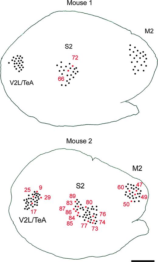
The fact that M2, S2 and V2L/TeA neurons varied monotonically in the parameters captured by the first PC suggested the possibility that the size of layer II/III pyramidal neurons is determined by the position of the neuron along the rostrocaudal axis in the cortex, since these three cortical regions vary in their position along this axis. To investigate this possibility we looked at the exact physical position in the cortex of the neurons, which were located at the edge of their respective clusters, in overlapping territories with neighboring clusters (Fig. 7). If the size of the basal dendritic morphology is influenced by the position of the neuron along the rostrocaudal axis, one would predict that the neurons which are statistically similar to the neighboring cluster should be located at the corresponding rostral or caudal edge of their own cortical region.
Location of the borderline neurons. Schematic drawing showing the sites of injection in the M2, S2 and V2L/TeA regions of the mouse cortex 1 and 2, as seen in the plane of section parallel to the cortical surface. Numbers indicate the exact position in the cortex of neurons. S2, V2L / TeA and M2 neurons that cluster outside their group and those located in the overlapping areas of the statistical map in Figure 6 are in red. These statistically similar neurons are not located in close proximity in the physical map, making a rostrocaudal gradient of morphologies unlikely. Scale bar = 815 μm.
Examination of the physical position of these overlapping neurons demonstrated, however, no apparent relation with the statistical position of the neuron along the PC axes (Fig. 7). Thus, the simplest interpretation of a gradient of morphologies, solely determined by the position of the neurons in the cortex, is not likely since there is no apparent correlation between the size of the neuron and its physical location within a region.
Discussion
Systematic Differences in Dendritic Morphologies among Different Cortical Regions
In this work we compared quantitatively the structure of basal dendritic trees from pyramidal neurons of three different and distant regions of the mouse neocortex. Our aim was to assess to what degree equivalent neurons in different cortical locations have similar morphologies and thus explore whether different cortical regions are built out of similar structural components. The strength of our study was to carry out an unbiased multidimensional statistical analysis of the data. Thus, the definition of what constitutes a neuronal class, which morphological parameters are important and how similar different cortical regions are, can be objectively approached in a multidimensional quantitative manner.
We find that layer II/III pyramidal neurons in each of the three cortical regions studied had a characteristic basal dendritic morphology. In both PCA coordinates and clustering trees, neurons from each cortical region are more similar to those of the same cortical region than they are to those of another region. V2L/TeA pyramidal neurons tend to have smaller and less complex dendritic trees than those of S2, and S2 neurons are on average smaller and less complex than M2 neurons. The fact that the first PC carries most of the variance and separates these three clusters of cells indicates that the size of the dendritic tree is the key factor differentiating these cortical regions. Our results therefore demonstrate that neurons of different cortical regions display characteristic morphologies. Despite considerable intra-regional variability, and the presence of outliers that cluster together with neurons in different zones, our data overwhelmingly demonstrate that the inter-regional variability is robust, to the point that it can be used to differentiate between neurons located in different rostrocaudal territories. Whether the intra-regional variability is related to cytoarchitectonic/functional differences within these territories remains to be determined.
These results agree with previous work that has emphasized differences in dendritic and spine morphologies among different cortical areas (Elston et al., 1997, 2001, 2005a,b; Elston and Rosa, 1997; Benavides-Piccione et al., 2002; DeFelipe et al., 2002; Elston and DeFelipe, 2002). We not only extend those findings to rodent cortex but also, for the first time, demonstrate them in a multidimensional analysis, blind to the chosen parameters, and also show that it is the size, rather than other topological aspects of the dendritic tree, that varies systematically.
Factors Determining the Morphology of the Basal Dendritic Tree
In addition, we also investigated the possibility that a rostrocaudal gradient of neuronal size is at work, whereby the position of a pyramidal neuron in the cortex could determine its size. This idea could account for the fact that the most caudal neurons, i.e. those of the V2L/TeA cortex, are also the smallest, whereas the rostral M2 neurons are the largest, and the S2 neurons, located in between, have intermediate sizes. The possibility of a morphological gradient could result from the existence of gradients of morphogens, something that has been clearly demonstrated in other parts of the developing nervous system (Drescher et al., 1997; Lee and Jessell, 1999).
Nevertheless, our analysis makes it unlikely that the systematic differences in morphologies that we have uncovered are the result of a simple rostrocaudal gradient. Although the physical position of the three groups of neurons in the cortex resembles somewhat the position of the three clusters of neurons in the statistical map based on PC axes, within each cluster, the detailed location of each neuron in the physical map does not bear similarity to its position on the statistical map. Moreover, when we specifically study neurons that cluster outside their group, we find that they are not physically located at the expected borders of their home areas.
Although we cannot rule out more complicated scenarios where several gradients are interacting, our analysis implies that the different morphologies are not the result of a simple monotonic gradient, but that instead each cortical site confers a distinct morphological identity on its neurons. The simplest interpretation is to assume that each cortical region is specified differently. This agrees with the genetic expression of particular factors, or combination of factors, in each cortical area (Rakic, 1988).
On the Structure of the Putative Canonical Microcircuit
How do our results impact the discussion of the canonical cortical microcircuit? By studying a selected type of neuron in three different regions, we demonstrate that each cortical zone appears to have a preferred morphological feature. The differences are quantitative and appear to be well captured by measurements of size. At first appearance, this result runs contrary to the strict interpretation of a canonical microcircuit, whereby each cortical area would be built by repetition of identical circuit elements. This view is not supported by our data or by previous studies in the tree shrew and various primate species which instead emphasize the idea that each cortical area possesses a tailored set of components (e.g. Elston, 2003; Elston et al., 2001, 2005a,b). Pyramidal cells constitute the majority of the total population of neurons in the cortex and are the source of the vast majority of inter- and intra- areal connections, (Jones, 1981; Felleman and Van Essen, 1991; Lund et al., 1994; DeFelipe and Fariñas, 1992). Thus, the structural differences found between cortical areas of the mouse must reflect differences in cortical process of information. For example, cortical neurons characterized by a smaller dendritic arbor must integrate inputs over a smaller region of cortex than larger cells. Furthermore, the integration of inputs leads to compartmentalization of processing within the dendritic arbors of pyramidal neurons. As a result, different branch structures undertake distinct forms of processing within the dendritic tree before input potentials arrive at the soma. Therefore, there may be a greater potential for compartmentalization in areas that contain highly branched pyramidal than in areas with less branched cells (for reviews, see Jacobs et al., 2001; Elston, 2003).
In summary, our data are in line with the idea that each cortical area is built from specific neuronal components. However, it is also clear that a number of microanatomical characteristics have been found in all cortical areas and species examined so far and, therefore, they can be considered as fundamental aspects of cortical organization. Given our still enormous ignorance about the exact number of cell types and connections in the cortex, future work will need to determine what is the nature of this essential kernel of cortical circuits and what are the specializations in the various cortical areas and species.
R.B.-P. thanks the ‘Comunidad de Madrid’ (01/0782/2000) and I.B.-Y. the MEC (AP2001-0671) for support. J.D. is supported by the Spanish Ministry of Education and Science (BFI2003-02745) and the Comunidad de Madrid (08.5/0027/2001.1). R.Y. thanks the NEI (EY11787) and the John Merck Fund for support and the Cajal Institute for hosting him as a visiting professor. We thank Guy Elston for training and members of the laboratory for comments.
References
Ballesteros-Yáñez I, Muñoz A, Contreras J, Gonzalez J, Rodriguez-Veiga E, DeFelipe J (
Bartfeld E, Grinvald A (
Basole A, White LE, Fitzpatrick D (
Benavides-Piccione R, Ballesteros-Yañez I, DeFelipe J, Yuste R (
DeFelipe J, Alonso-Nanclares L, Jon I. Arellano JI (
DeFelipe J, Fariñas I (
Douglas RJ, Martin KAC (
Douglas RJ, Martin KAC (
Douglas RJ, Martin KAC, Whitteridge D (
Douglas RJ, Koch C, Mahowald M, Martin KAC, Suarez HH (
Douglas RJ, Martin KAC, Markram H (
Drescher U, Bonhoeffer F, Muller BK (
Elston GN (
Elston GN, Rosa MGP (
Elston GN, DeFelipe J (
Elston GN, Pow DV, Calford MB (
Elston GN, Benavides-Piccione R, DeFelipe J (
Elston GN, Benavides-Piccione R, DeFelipe J (
Elston GN, Elston A, Casagrande V, Kaas JH (
Escobar MI, Pimienta H, Caviness VS Jr, Jacobson M, Crandall JE and Kosik KS (
Felleman DJ, Van Essen DC (
Fleischhauer K, Petsche H, Wittkowski W (
Franklin KBJ, Paxinos G (
Frost D (
Gilbert C, Wiesel TN (
Hubel DH, Wiesel TN (
Hubel DH, Wiesel TN (
Jacobs B, Schall M, Prather M, Kapler E, Driscoll L, Baca S, Jacobs J, Ford K, Wainwright M, and Treml M (
Jones EG (
Katz LC, Shatz CJ (
Kozloski J, Hamzei-Sichani F, Yuste R (
Lee K, Jessell T (
Lorente de Nó R (
Lund JS, Yoshioka T, Levitt JB (
Mountcastle VB (
Nimchinsky EA, Gilissen E, Allman JM, Perl DP, Erwin JM, Hof PR (
Peters A, Walsh TM (
Peters A, Yilmaz E (
Ramón y Cajal S (
Rockel AJ, Hiorns RW, Powell TPS (
Sur M (
Tsiola A, Hamzei-Sichani F, Peterlin Z, Yuste R (
Author notes
1Instituto Cajal, Madrid, Spain and 2HHMI, Department of Biological Sciences, Columbia University, New York, USA