The Modeling of Shock-Wave Pressures, Energies, and Temperatures Within the Human Brain Due to Improvised Explosive Devices (IEDs) Using the Transport and Burgers' Equations
 Stephen W. Mason
- Mathematical Researcher, Leeds, United Kingdom
This second paper adopts a more rigorous, in-depth approach to modeling the resulting dynamic-pressures in the human brain, following a transitory improvised explosive device (IED) shock-wave entering the head. Determining more complicated boundary conditions, a set of particular-solutions for both Burgers' and the Transport equations has been obtained to describe the highly damped neurological pressures, complete with respective graphical plots. Many of these two-dimensional solution-curves closely resemble the Friedlander curve [1–4], not only illustrating enormous over-pressures that result almost immediately after the initial impact, but under-pressures experimentally depicted in all cases, due to oscillatory motion. It appears, given experimental evidence, that most—if not all—of these models can be aptly described by damped sinusoidal functions, these facts being further corroborated by existing literature, referencing models expounded by Friedlander's seminal work [1–4]. Using other advanced mathematical techniques, such as the Hopf-Cole Transformation, application of the Dirac-delta function and the Heat-Diffusion equation, expressions have been determined to model and predict the associated energies and temperatures within this paper.
Introduction
In Paper 1, a one-dimensional model of the human head, through which a shock-wave due to an improvised explosive device (IED) blast traveled, was developed. Within this scenario, the initial shock-wave was modeled with a partial differential equation (PDE) known as Burgers' equation and, from the assumed initial boundary-condition, several shock-wave solution-curves were graphically plotted using experimental data derived from existing literature. It was hoped that, given this primary data, the theoretical calculations would match the experimental observations. Thus, future predictions about as-yet unknown IED neurological shock-waves should be possible. In setting up the preparatory conditions to tackle the challenges of this paper, it was indicated that the sheer violence of the shock-wave may have significantly harmful effects upon the human brain during and after battle, and a physics-based discussion about some of these issues followed.
In addition to high-velocity longitudinal pressure-waves, observed to cause significant brain trauma, it is mentioned that shear—or transverse—waves can be explained by similar physics-based mathematics, in terms of the way in which waves behave during their propagation through the brain.
In continuing this mathematical discourse, we turn to further worked solutions of Burgers' equation by first considering damped sinusoidal motion of the resulting, dynamic, variation in pressure following initial transitory shock-wave propagation through the human head.
Modeling of Variation of Pressure in Terms of u(t, x)
From each of the Equations (19) and (20) in Paper 1, the resulting second-order Burgers' equation is obtained as expressed in Equation (16). When γ ≅ 0, Equation (16) reduces to the first-order Burgers' equation. In each of these two cases, one can see that the non-linearly varying pressure can be expressed solely in terms of u(t, x) and its derivatives.
From the results outlined by Mediavilla et al. and Moore et al. [5, 6], one can assume that decreases (or increases) in the observed pressure can be modeled by an exponentially decreasing sinusoidal curve of either of the form e−ωxsin (ωx) ore−ωxcos (ωx). Here, the Cauchy Problem has again been adopted, whereby each of these latter boundary conditions satisfies its requirements, outlined within definition 1, in Paper 1.
A Friedlander-Type Model of Pressure-Variation
Commencing with Equations (16), (17), and (26) of Paper 1, and following through with the previous working, we find:
as before. Assuming c = 0, we have:
By observing the experimentally obtained graphs, the decreasing- sinusoidal pressure-waves can be conveniently modeled by applying either of the functions representing the most appropriate boundary conditions:
or:
yielding the maximum (or minimum) pressure at some non-zero value of x (and t, usually approximated to zero) after impact. Using calculus to determine such maximum and minimum pressure values, either Equation (51) or (52) may model the given observations appropriate to the underlying physical situation, whereby α and β are constants of proportionality, and are determined by the parameters involved.
From the above boundary condition, since the initial pressure is represented by u(0) = 0, we see this satisfying the zero-pressure outlined in the experimental results of Moore et al. [6].
However, the pressure at x = 0.176 m is also taken to be zero. Thus:
Assuming e−ωx ≠ 0, we deduce that , such that both boundary conditions at x = 0 and x = 0.176 are satisfied. In this case, we see that ω is expressed as integer values, n, of the angle, , for n = 0, 1, 2,.…For simplicity, we can set n = 1, thus obtaining a single wave whose angular-frequency is .
Keeping ω in its present form, for the first boundary condition, we can write Equation (51) as:
Since experiments show that neurological pressure decreases in magnitude as time increases—where x is fixed and t is large—we can assume from Equation (23) of Paper 1, that the characteristic, k, and therefore, ωk, is ultimately very small, such that:
By applying the Cauchy Problem in definition 1 and expanding both e−ωk and sin (ωk) each, as k → 0 and t → ∞, as in the subsection Elementary Model for Pressure-Wave With Simple Undamped Sinusoidal Function, we find that the product of these two functions can be approximately written:
Assuming γ = 0, such that c = 0, then the third ODE from Equation (26) becomes:
yielding:
As Moore et al., [6], pointed out, their description of their shock-tube experiments indicated that the initial neurological pressure-wave was delayed by and s for both tensile and compressive peak-pressures of 6.5 MPa and 0.89 MPa respectively, making the average time-phase for each of these occurrences s after the initial shock-wave impact. The average spatial-phase shift for each of these maximum pressures for a 5 m/s impact simulation [6], is 2.325 × 10⁻³ m, which is equal to just over a millimeter. For example, the shock-wave peaked at this fractional time somewhat discontinuously, after propagating through m of brain tissue, apparently at standard pressure levels. Therefore, these two statistics may be used as the shift in the phase-angle, to correctly, and as accurately as possible, model the whole motion.
By using the mechanics of a wave shifted toward the right-hand-side, Equation (58) can be re-written as:
and substituting Equation (56) into this, we obtain:
or:
becoming:
Substituting this last affine characteristic equation into the solution gives:
Likewise, adoption of the boundary condition illustrated by Equation (52) yields:
Note that, although Equations (63) and (64) are partially expressed as quotients of the units of space divided by the units of time, each equation nonetheless satisfies the definition of the Cauchy problem in definition 1 of Paper 1. This is because either of the functions still remains analytic at the initial time, t = 0, yielding specific maximum pressure values solely in terms of x at this point, whereby u(0, x) = u(x), as necessary and required.
Determination of the Value of Constants of Proportionality, α and β, and Maximum Pressure, PM
As before, considering limits, we find that the boundary condition at x = 0 yields zero pressure, or u(t, x) = 0, and at x = 0.176 m the pressure is also approximately zero as t → ∞. The conclusion is that .
Substituting the general variate k, into Equations (51) and (52) respectively, we obtain:
and:
each of which can be differentiated to obtain the peak values at uk(k) = 0:
and:
Solving Equations (67) and (68) separately yields two trigonometric functions for each:
and:
Since for both Equations (69) and (70) respectively, they each yield the respective values of k as and 0.0848647….
Given that the peak-pressures for u(k) occur at the above two values for k and can be represented by some value, PM, at these points, by substituting and k = 0.085 into Equations (65) and (66) respectively, they become:
or:
leading to:
and:
Therefore, Equations (65) and (66) can be written:
and:
Using Burgers' equation to model a propagating incident pressure-wave with a peak value of u(T, L) = 30, 000 Pa, for example, where T = 4.65 × 10⁻⁴ s and L = 2.325 × 10⁻³ m at 30,000 Pa [5, 6], initially obtaining Equations (75) and (76) by the above analytical methods, indicates, for a calculated maximum value of PM ≅ 30,000 Pa, the solution shown in Figure 7A below. It is notable that, after the shock-discontinuity, this pressure-curve does not appear to display a negative-phase—otherwise referred to as an under-pressure—but, unlike Figure 7B, it is a non-linear wave since A(k) = u(t, x) is a variable coefficient (and a function of the independent variables, t and x) of the ux term in the original Burgers' equation. However, as t increases indefinitely, the pressure wave monotonically converges to the normal atmospheric base pressure-level (taken to be zero), as observed by Mediavilla et al. [5].
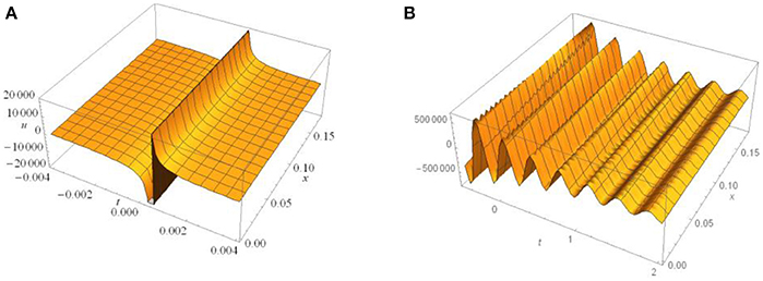
Figure 7. (A) The plot of vs. t and x. Note here that t commences at 0 s and runs to 0.04 s, with x ranging from 0 to 0.176 m. As t approaches an infinite value, the pressure, u(t, x), monotonically decreases to zero with respect to both axes. These factors are consistent with the limiting value of u(t, x), in which x is fixed as opposed to infinitely increasing time, t. (B) Plot of the linear wave, . In this graph, since the angular-frequency, ω , has been omitted in the exponential factor, it is evident that the wave is now periodic in the t-direction as compared to the plotted monotonically decreasing wave in (A). Note here that t commences at 0 and runs to 2 s, with x ranging from 0 to 0.176 m. As t → ∞ , the pressure-oscillations gradually become damped out to zero.
In the case of the Transport equation (or the linear Burgers' equation) solution, however, illustrated by Figures 7B, 10A,B, it is evident that the variation in pressure-values, u(t, x), especially according to the different wave velocities represented by c over the given ranges 0 ≤ x ≤ 0.176 m and 0 ≤ t ≤ 0.004 s, descend into negative values for various parameter values, respectively, after a certain point over the range 0.002 ≤ t ≤ 0.004 s, [5–7]. This solution also describes negative under-pressures reasonably consistent with published literature and, although the theoretical graphs in this publication are not completely identical to their experimental counterparts, there are still considerable similarities and trends—for example: general shape, periodicity, and convergence with increasing time.
By analyzing each graph below, one observes that the higher the wave-velocity, c, the sooner the maximum pressure, u(t, x), occurs in all cases and is often of a higher value. This latter feature is especially true when all the reflected waves in Figure 10A are added together and then re-plotted as a single wave, illustrated in Figure 10B. For different wave-velocities, more appropriate values of α (and β) can be found, via calculus and algebra, so that observed graphical peak pressures yield their respective values as witnessed during experimental observations.
Returning to Figure 7A, it appears that the pressure is largely constant along the x-axis, due to the spatial coordinate being fixed—and therefore effectively static—although non-linear with respect to t, over the given limits. This graph, illustrating a solution for the Burgers' equation, is again non-linear. In Figure 7B, there is similar spatially-axial behavior, except for the periodicity and the presence of under-pressures with-respect-to time, the latter of which [8] suggests may be due to compression of the skull and recoil of the brain. However, the graph's solution-curve—like the Transport equation from which it is derived—is linear, as will be described in the section Preamble to Cauchy Problem when the equation is solved. A fuller picture of either graph's behavior would be obtained by considering longer-term analysis of the variables; variability becomes more obvious, especially within the dynamic-based models as part of the Mathematica software.
In some of the Transport equation solutions in Figures 10A,B, below, it is easier to see that u(t, x) is often negatively valued between 2 and 5 ms, but then becomes slightly positive whilst converging to zero pressure with increasing time. Very similar results for the data used in this research were recorded by Mediavilla et al. and Moore et al. [5, 6], whose pressure-time graphs exhibited negative values of u(t, x) between the above limits in many cases.
As the experimental results further indicate, the plotted graphs within this research sometimes show the presence of under-pressures, as in Figures 7A–10B, immediately after a shock-wave's instantaneous entry into the brain up to the point of discontinuity. At the time, the reasons for these apparent under-pressures were not clear, [8], but can be described, not only by application of more appropriate sinusoidal boundary conditions shown below, but also because of the reflection and transmission coefficients associated with each wave rebounding within the skull and brain. For example, it is known that when impact waves are reflected from a surface, they often display a trough immediately after rebounding (as opposed to the original incoming peak) due to the nature of the reflection coefficients (Paper 1) and energy considerations. Even if implicitly related, reflection of such waves could be associated with both initial and subsequent under-pressures—at either side of a given parameter on the t − x axes—whereby there does appear to be a link. Mediavilla et al. [5], also state that “the initial pressure in the gelatin becomes negative (in the first 0.5 ms); after which it follows the surrounding air pressure within the tube. The reason for this pressure drop might be due to experimental setup, since a new series of experiments did not show this effect”. The authors' assertions here could be correctly founded, given that any phase difference in an emitted wave, possibly due to differing experimental setup, could conceivably affect the periodicity of the incoming, transmitted, and reflected waves' peaks and troughs. As suggested above, this may further tie in with the compression of the skull and recoil of the brain, [8], but in ways that are dictated by the physical positioning and directional nature of both the apparatus and the emitted waves, respectively. If this is so, then one could potentially explain either the presence or absence of apparently inconsistently occurring under-pressures that were previously unexplained.
Pressure-Time Solution-Curves for Different Maximum Pressures and Boundary Conditions Closely Resembling the Friedlander Curve
The constant of proportionality, ω, in the exponential term of Equation (75), is of small consequence and, in Figures 8A,B, the graphs of this equation indicate the presence of very slightly less acute discontinuities, compared to those in the second series of pressure-profiles in Figures 9A,B, as modeled by Equation (76). Both sets of curves are close fits for the experimental data, describing the apparently misunderstood physics. All these profiles seem to resemble aspects of the Friedlander curve, [1–4], particularly for a range of modeled incident pressures commencing at 30,000 Pa and higher over given spatio-temporal ranges. The time ranges have been chosen so that both sets of graphs may be compared, and because they indicate similar times observed within current shock-tube literature. Sometimes, however, shorter spatio-temporal ranges have been chosen here for the purposes of illustrating clearer and more discernible solution curves. This should be considered when comparing them with other authors' findings.
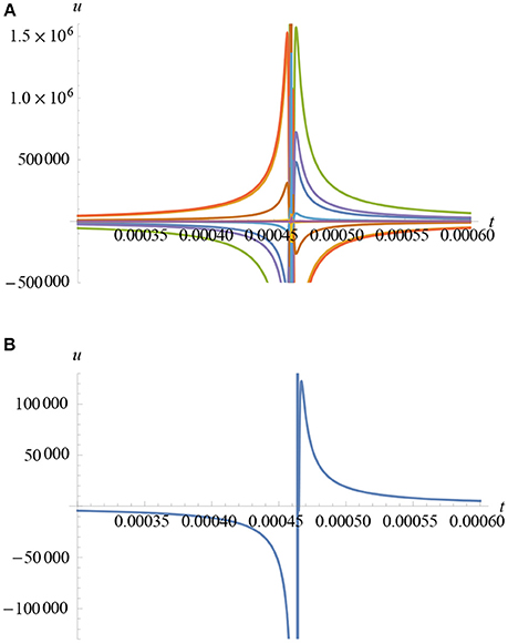
Figure 8. (A) The variation of wave-pressure vs. time for a series of different transmitted and reflected waves described by Equation (75). (B) The variation of wave-pressure vs. time for the superposition of each of the waves in (A) there is a chaotic region of highly alternating pressure close to t = 0.00045 s.
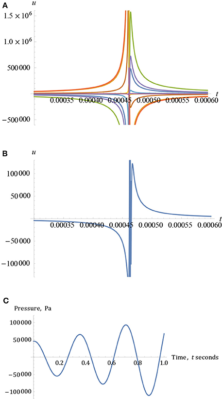
Figure 9. (A) The variation of wave-pressure vs. time for a series of different transmitted and reflected waves described by Equation (76). (B) The variation of wave-pressure vs. time for the superposition of each of the waves in (A) there is a chaotic region of highly alternating pressure close to t = 0.00045 s. (C) The variation of wave-pressure vs. time for , for a shear wave-velocity of 4 m/s and temporal-phase, t0. The solution blows-up given that , as t → ∞, where is both fixed and finite, and is eventually exceeded by this increasing temporal-variable, t.
Introduction to Smoother and More Continuous Friedlander-Type Solution-Curves Illustrating Observed Under-Pressures
By considering a wider range of parameters, more accurate solutions of the observed under-pressures can be calculated, providing reasonably appropriate descriptions of this phenomenon. Since the transverse components of a pressure-wave can also be equally as damaging to such as axons and white matter, [6], their respective shear wave-velocities, such as c = 4, 10, and 30 m per second, [5], yield some of the two-dimensional graphs in Figures 10A–16A, in which the peak-pressures occur sooner when the shock-wave impact-velocities are higher. For example, this becomes especially noticeable when substituting longitudinal velocities—of a factor of 100 times or more than the shear ones above—into the Transport equation solution, again illustrated by Figures 10A,B. Furthermore, they provide examples that the inherent mathematics of each situation automatically dictates both over- and under-pressures, often (if not always) to be observed and certainly to be expected.
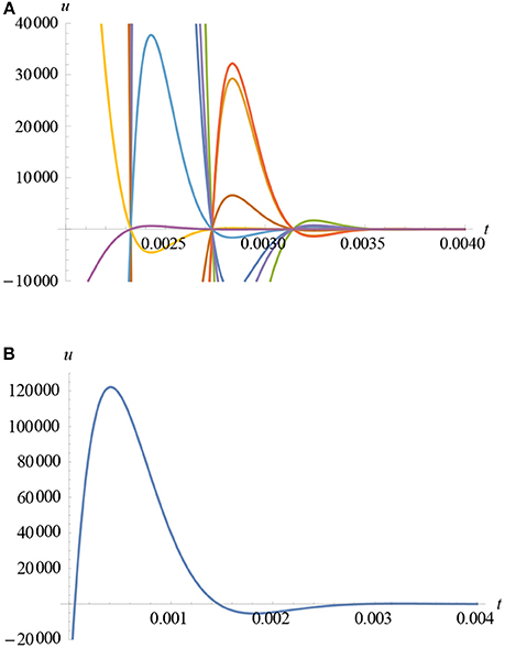
Figure 10. (A) The variation of wave-pressure vs. time for differing wave-velocity: higher velocity waves peak sooner than those of lower velocity (some curves have been omitted for clearer visibility). (B) The variation of wave-pressure vs. time for the superposition of each of the 40 m/s waves in (A). Here, after the point where the curve first becomes positive, the maximum peak-pressure is 122,192 Pa and the minimum is −5280.39 Pa (−0.052 atm).
In addition, further shock-tube experiments have been developed for shock-wave velocities of 40 m per second and higher, by authors such as [5], as shown in Figures 7A–10B.
These two-dimensional graphs of u(t, x), for the various values of c, have again been plotted with respect to t (but with the latter x variable fixed, x ≤ 0.176); each of them displays a smooth and non-periodic pressure-curve, as plotted from the derived general solutions:
and:
Each of the plotted pressure-curves for these two equations represent some appropriately calculated values of the effective maximum pressures, for various values of α and β , whereby:
and:
which are associated with the respective velocity, c, of the traveling shock-wave. Both Equations (77) and (78) are derived in the subsection Approximate, Smoother and More Continuous Forms of the Friedlander Curve to model Pressure Versus Time from Initial-Boundary-Conditions, and their solutions plotted respectively.
Further Analysis of Pressure Curves
Mathematical analysis shows that, in Equation (75) for example, the minimum and maximum pressures oscillate between the values of approximately −PM and PM close to the discontinuity at the point where t ≅ 4.65 × 10⁻⁴ s. Therefore, regardless of the small, fixed, value of x, we find that as t → 4.65 × 10⁻⁴ s, then k → ∞ , and so u(t, x) passes through u = 0 Pa between the pressures of −PM and PM at least once. Due to this multiply valued (and highly oscillatory) condition of the function's value at this point, it fails to converge to a limit here. This explains why one first observes an under-pressure between the origin and the discontinuity at t = 4.65 × 10⁻⁴ s—as can be witnessed from the green curve in Figure 8A—and then an overpressure thereafter ultimately decaying, exponentially, with increasing time. Similar analyses can be carried out on Equation (76) yielding slightly more complex results as shown in Figure 10B.
The last analytic and graphical feature, described above and explained further in this section, indicates that the apparent occurrence of initial negative pressure magnitudes, or under-pressures, are also inherent physical factors within this area of science, especially from the viewpoint of certain mathematical models. Within the literature, they have normally been explained as features associated with erroneous experimental methodology, [5, 6], but this is not necessarily the case. Whilst there may be issues surrounding this suggestion (for example, those affecting the phase of a transmitted wave resulting in the presence of inconsistently occurring under-pressures, as mentioned earlier), the negative under-pressures, illustrated by the graphs up to the occurrence of the discontinuity in both Figures 8A,B, 9A,B, are largely due to the underlying universal physical laws of shock-wave mechanics associated with this area of neurological dynamics. The given PDE s, such as Burgers' and the Transport equations, are fundamental in describing many aspects of the experimental observations, including the parts played by the inherent sinusoidal motion and conservation laws, which would otherwise be insufficiently understood—if at all—for making significant advances.
Proof By the Characteristic Method—an Initial-Boundary Value Problem
Two alternative solutions to Equations (75) and (76), as illustrated above, are Equations (77) and (78), derived as follows. It is intended that they will supplement what has already been discovered, whilst simultaneously offering a different perspective to this area of shock-wave dynamics. There are certainly similarities between all the plotted solutions in this section and the section Boundary Conditions Within a Typical Case, but there are other facets that each group illustrates more convincingly, compared to the other. In short, both sets of solutions have strengths and weaknesses; where one fails to illuminate, the other does.
For a wave traveling to the right-hand-side, the wave-velocity can be expressed in two possible Galilean ways, namely:
and:
Equation (81) was used in the sections from Appropriate Boundary Condition Leading to a Characteristic Solution in the Case of a Shock Wave to Elementary Model for Pressure Wave With Simple Undamped Sinusoidal Function, and Equation (82) has been adopted in this section, largely because it adopts a more appropriate relativistic-time-shift (measured in seconds), given that aids in the calculation and plotting of pressure vs. time, which is largely in the graphical format adopted by experimental observation. Had we needed to calculate the pressure vs. distance solutions, then Equation (81)—in which the relativistic-distance-shift in terms of the spatial co-ordinates, (x − ct), is important—would have been adopted instead.
To plot each of the two-dimensional graphs, in Figures 8A–10B as accurately as possible, we must solve the above problem by considering the wave-profile whose maximum pressure characteristics are further shifted by a factor of t = 4.65 × 10⁻⁴ and x = 2.325 × 10⁻³ m along both axes, respectively. For example, as Mediavilla et al. [5] observe, the analysis within this research further shows a discontinuous jump in pressure from 0 Pa to a maximum, PM, for each profile at these values of t and x. Partially using data gleaned from Moore et al. [6], this feature has been recreated by substituting an appropriate expression for the characteristic variable, k, into the boundary conditions in Equations (51) and (52), namely:
and:
Approximate, Smoother and More Continuous Forms of the Friedlander Curve to Model Pressure vs. Time From Initial-Boundary-Conditions
As much literature indicates, a solution-profile of a pressure-wave is often most appropriately modeled by the Friedlander curve, [1–4]. This section of the research demonstrates that this area of shock-wave physics, modeled by both the non-linear Burgers' equation, and its linear version, the Transport equation, yields very similar theoretical results to those observed during experimentation.
By commencing, this time, with the linear form of Burgers' equation—or the Transport equation—in which u = A(k) = c, we have:
and following through with the integration as in the section Determining General Boundary Conditions in Each Case, we find:
Since we now model the given situation with regards to the initial-boundary conditions, we must introduce a dummy variable, s, into the system of the three ODEs representing the characteristics. The initial conditions are written as t0(s) = t0, and x0(s) = x0, and a slightly different approach to solve this problem—compared to those previously employed in the sections Burgers Equation Derivation in Terms of Velocity and Pressure—Simplified Result of Navier-Stokes Equation and Boundary Conditions Within a Typical Case—will now be adopted.
We commence with:
As in the sections Boundary Conditions Within a Typical Case and Modeling of Variation of Pressure in Terms of u (t, x), we write the ODEs separately, divide each one by the dummy variable, ds, and equate to unity. Rather than complicating matters, this procedure simplifies the process, since all one needs is to integrate the equations with respect to ds. The purpose of applying this approach is to allow three separate solutions, one in terms of t(s), the other in terms of x(s) and the third in terms of u(s). At the end of the exercise, application of the initial conditions will show that s = k, which helps to simplify the end result.
As above, we write:
When t(s) = t0, , each of these ODEs yield, in turn, the results:
and:
and, since μ = 0, separating out the variables and solving, we have:
Since in Equation (86), where k is the constant-valued intercept of the linear characteristic with the x-axis when s = 0 at t = t0, each of the Equations (85) and (86) becomes:
respectively or, for easier calculation, Equation (91) may be written:
Substituting Equation (90) into Equation (92) results in:
then, dividing both sides of Equation (93) by c, we have:
or otherwise:
In Equation (95), we see that k is clearly linear, regardless of the values of t and x (where x is fixed), and we only require the phase-shift for the pressure-wave to be written in terms of t0, and not x0, due to the linearity of the system as defined by the Transport equation. One may graph the solution-curves with respect to the spatial-axis as well, in which only the spatial phase-shift, x0, is required, and not t0, largely depending on the nature of each solution that one requires. These latter features are illustrated below, in which Equation (95) has been regularly used as the independent variable in the plotting of a number of profiles for the pressure-waves as they propagate with respect to time, t, as commensurate with the literature. The formula will also be derived to plot the pressure-wave with respect to x, should it be required for scientific analysis.
To summarize the above analysis, given the linear Transport equation has been employed as required, to model a range of shear-wave velocities, c = 4, 10, 30, 40 m/s, along with longitudinal velocities such as 1,463 m/s, [5], for example, the above analysis often demonstrates no change in the spatial-axis as t increases, although the pressure itself does vary with time even at fixed values of x. For example, compare taking a snapshot of the pressure-wave at a fixed and static value of x, whereby the wave only propagates with respect to the time-axis.
Substituting Equation (95) into Equation (82) for the required boundary condition, we have:
in which only the temporal-phase shift in t0 is shown. Hence, a solution still propagating only with respect to time, t, where x is fixed, is thus considered.
We can also write Equation (96) as:
We now re-work the whole Cauchy Problem, but this time only considering the spatial-shift, x0, for a pressure wave propagating with respect to x, along with the initial condition . From Equations (87) and (88), we write k = t−s and and then, substituting the latter expression into the former for time, we obtain:
as before, such that:
For the time-phase solutions, if we substitute Equation (95) into each of the boundary conditions, Equations (51) and (52), we have:
and:
in which only the time-phase, t0, and thus the propagation of the pressure-wave with respect to time, only, for fixed x, is now evident. A typical solution for the pressure-wave of 30,000 Pa, as given in Equation (101) —in which the indicial angular-frequency, ω, is absent—and with a shear-wave velocity of 4 m/s, is shown in Figure 9C below. A further analysis showing the pressure appearing to blow up as t increases, indefinitely, is explained at the end of the section Use of the Cauchy Problem to Determine More Appropriate Spatial Boundary Conditions for Shock-wave Solution for a similar curve, in which the shear wave-velocity is 40 m per second.
For solutions involving only the spatial phase, x0, and the subsequent propagation of the pressure-wave with respect to x, for fixed t, then we substitute Equation (97) into Equations (51) and (52) to obtain:
and:
Note that Equations (100)–(103) differ, slightly, from the more intuitively formed functions of (106) and (107) below, in which the temporal phase-shift along the t-axis was simultaneously considered alongside the spatial phase-shift with respect to the x-axis. However, although the intuitive approach does not always greatly affect the outcome of the solution-curves, in this individual case—for small values of time, t, and due to the vanishingly small magnitude of the temporal phase-shift—strictly speaking, it is incorrect. This is due to the above explanations regarding the wave's linearity.
Again, by adopting the proper analysis, one can take a relevant snapshot of the propagating wave, either with respect to the t-axis or with respect to x, depending on the model required, but not simultaneously, since neither of the phase-factors occur together if one adopts the above (correct) analytical approach. Ideally, one should only ever use the correctly derived analytical case, as the intuitive version often fails to yield the correct analysis and can be considerably misleading.
As discussed above, one can think about this Transport problem without considering the Cauchy Problem. Although not as analytically correct since the time-phase magnitudes are so vanishingly small, their presence in the solutions, below, make virtually no difference to the outcome of the analyses.
To illustrate the potential shortcomings of the intuitive approach, we proceed as follows, and write the general solution as:
Therefore, given the actual two possible boundary conditions in Equations (51) and (52), namely:
and:
then each of these expressions can be written more explicitly:
and:
As usual, the temporal and spatial coordinates are transformed by the vanishingly small temporal-phase of 4.65 × 10⁻⁴ s and the spatial-phase of 2.325 × 10⁻³ m, so the characteristic variable, k, can now be re-written:
which simplifies to:
Substituting the characteristic Equation (110) into either of the boundary conditions, Equations (65) and (66), we obtain the solutions:
and:
In these latter two equations, and as explained above in the section Determining General Boundary Conditions in Each Case, the time phase in these is so vanishingly small that it effectively reduces each expression to the solution illustrated in Equation (101) in the section Approximate, Smoother and More Continuous Forms of the Friedlander Curve to model Pressure Versus Time from Initial-Boundary-Conditions. It may be concluded that there would be no substantial difference in the graphical curves for any of the three if they were to be plotted with the inclusion of this temporal-factor, although the problem of “blow-up” of their solutions materializes as time increases without bound, as shown in Figure 9C. This is at least one modeling problem in the case of a system in which convergence is required.
By first plotting Equation (102) separately for successive constant, maximum-valued, reflection coefficients, R = 0.555, defined by the Power Series from Paper 1, the latter of which is stated here again:
we obtain the profiles in Figure 10A, below. Here, we have substituted various test velocities representing c, such as 4, 10, 30, 40 and 1,463 m/s, each corresponding to multiples of the frequency of around 7,700 Hz, [5], with the same initial maximum incident pressure of 30,000 Pa for each situation. Detailed inspection of each graph, along with appropriate mathematical analysis—as each successive higher velocity is applied with its corresponding wave-frequency variations—shows the phase-angle along the t-axis decreasing. This means that maximum pressure, PM, occurs sooner, after the point where it first becomes positive. The underlying physics is true, regardless of what the subsequent maximum pressure in each case happens to be. However, when reflection coefficients are applied, the respective maximum pressure either increases or decreases (due to constructive and destructive superposition) depending on the wave component of the sequence and the extent of the superposition applied. Figure 10B shows the total sum of all the individual superimposed reflected waves described by Equation (102) for a 40 m/s test-velocity, assuming that the reflection coefficient of R = 0.555 is still applicable. It also demonstrates why IED shock-wave mechanics often results in greatly magnified pressures within the brain, post-shock. In this case, the magnification yields just over four times the initial 30 kPa incident pressure up to the peak-value of 122,192 Pa at around 0.4 ms, before decaying as time increases. This is to be expected given the four-fold calculation of the previous reflection-coefficient theory in Paper 1. It is also found that the minimum value is −5,280.39 Pa, or 0.052 atm (0.052 bar) below normal brain-pressure, at around the value of t = 1.8 ms after the initial shock-wave impact, before rising again slightly, and converging to a normal level.
It has to be noted, here, that consecutive reflection-coefficients are likely to decrease in magnitude every time the wave rebounds from each side of the skull due to the successive reductions in wave-velocity or frequency. This means that maximum and minimum brain pressure will differ, in reality, from that calculated for the constant and unchanging value of R = 0.555 in this particular case.
It is also worth mentioning that, unlike the solution-curves in the section Pressure-Time Solution-Curves for Different Maximum Pressures and Boundary Conditions Closely Resembling the Friedlander Curve—in which the time-phase is vanishingly small with s—the time-phases in Figure 10A are much greater by comparison, especially at low velocities, c. These factors are a combined result of other parameters inherent in the method of solution, ultimately taking into consideration initial-boundary-conditions whilst also explaining the under-pressures between around 2 and 5 ms, as observed in shock-tube experiments [5, 6].
Negatively-Damped Decreasing Sinusoidal Pressure-Curve Solutions
By applying Equation (103), which does not involve the factor of ω in the exponential term, instead of obtaining a smoothly decreasing curve, one now obtains the oscillatory, and therefore periodic, amplitude-decreasing profiles in Figures 11A–C. This negatively damped feature of the solution-curve is due to the exponential term approaching zero magnitude, therefore causing the observed, more gradual, decay. Again, if one plots Equation (100), the exponentially increasing term (for ct > x) causes positive damping and the subsequent rapid blowing up of each oscillatory solution for an unbounded, indeterminate length of time. This latter fact is largely due to the positions of t and x, relative to each other in the exponent, leading to positive indicial values after the point where ct = x. In combination with the sinusoidal term, this positively increasing exponential term causes the oscillatory nature of the solution to vary wildly, as shown in both Figures 12A,B below. As explained in the section Proof by the Characteristic Method—an Initial-Boundary Value Problem regarding the similar, but more gradual, positive damping effects of Equation (101) and its solution curve, Figure 9C, the pressure cannot increase indefinitely, largely due to the conservation laws. However, the analysis of this theory may also further explain the physics occurring during experimental observations regarding apparent increases in pressure magnitudes.
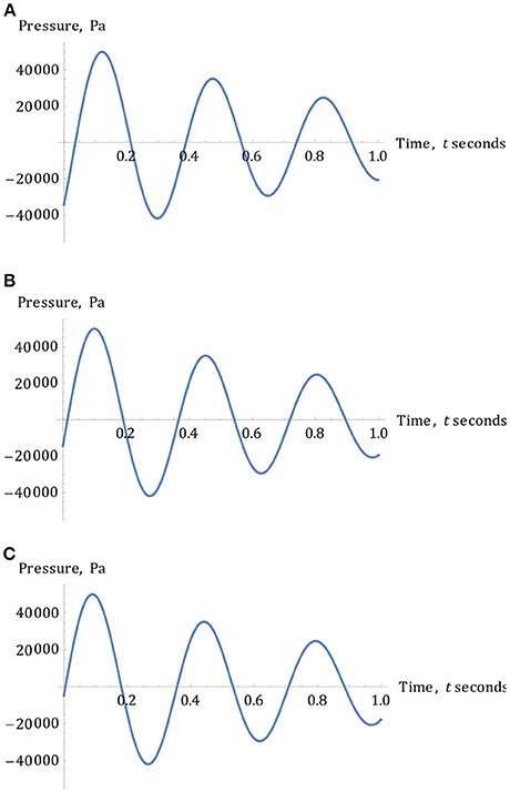
Figure 11. (A) The variation of wave-pressure vs. time for a wave-velocity of 4 m/s. (B) The variation of wave-pressure vs. time for a wave-velocity of 10 m/s. (C) The variation of wave-pressure vs. time for a wave-velocity of 30 m/s.
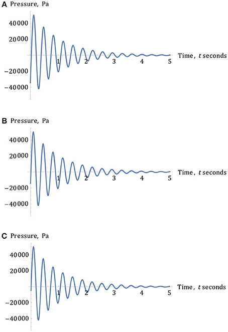
Figure 12. (A) The variation of wave-pressure, PM = 50, 000 Pa, vs. time for a wave-velocity of 4 m/s over the time interval of 0 ≤ t ≤ 5 s. Note the rapidly decreasing profile, complete with both under-pressures and over-pressures. (B) The variation of wave-pressure, PM = 50, 000 Pa, vs. time for a wave-velocity of 10 m/s over the time interval of 0 ≤ t ≤ 5 s. Note the rapidly decreasing profile, complete with both under-pressures and over-pressures. (C) The variation of wave-pressure, PM = 50, 000 Pa, vs. time for a wave-velocity of 30 m/s over the time interval of 0 ≤ t ≤ 5 s. Note the rapidly decreasing profile, complete with both under-pressures and over-pressures.
Also, for all these less-damped sinusoidal curves, when velocities, c, increase with greater magnitude, the onset of the initially increased pressures, and their subsequently damped oscillations, again occur more closely to the origin, just as they do for more heavily damped cases, in each successive case.
By increasing the time-interval between 0 and 5 s, over which the pressure-wave propagates, one can see the convergent nature of each more clearly over this longer duration, whilst keeping x fixed at 0.176 m. The graphs representing each of these test velocities of 4, 10, and 40 m/s, once again, with the same maximum pressure, PM = 50,000 Pa, appear to yield considerably decaying pressure-waves in each of the Figures 12A–C. The corresponding profiles for a velocity of 40 m/s, as used by Moore et al. [6], are plotted in Figures 13A,B.
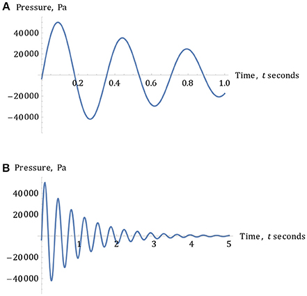
Figure 13. (A) The variation of wave-pressure vs. time for a wave-velocity of 40 m/s. (B) The variation of wave-pressure for a wave-velocity of 40 m/s over the time interval of 0 ≤ t ≤ 5 s. Note the rapidly decreasing profile, complete with under-pressures and over-pressures.
In the above figures, it is evident that the variation in pressure-values, u(t, x), especially given the three-different test wave-velocities, c = 4, 10 and 30 m/s over the given ranges, 0 ≤ x ≤ 0.176m and 0 ≤ t ≤ 0.5 s, descend into negative values, respectively, after a certain point. By analyzing each graph in Figures 13A,B above, one observes that the higher the wave-velocity, c, the higher the initial maximum pressure, u(t, x), appears to be in many cases. For different wave-velocities, more appropriate values of α can potentially be found, via calculus, so that observed graphical peak pressures yield their respective values as witnessed during experimental observations.
Whilst analyzed in simultaneous combination with the spatial phase in Equations (110) and (112) in the section Approximate, Smoother and More Continuous Forms of the Friedlander Curve to model Pressure Versus Time from Initial-Boundary-Conditions, when taken on its own, the temporal variable and phase—in the absence of the spatial version—could be partially responsible for experimentally observed increases in pressure magnitudes within the brain, after the initial, transitory shock. However, other factors, such as parabolic reflection, may be a concomitant factor in this respect. One should consider that, due to conservation issues previously mentioned, the pressure cannot increase indefinitely, as appears to be the case in Figures 14A,B, above.
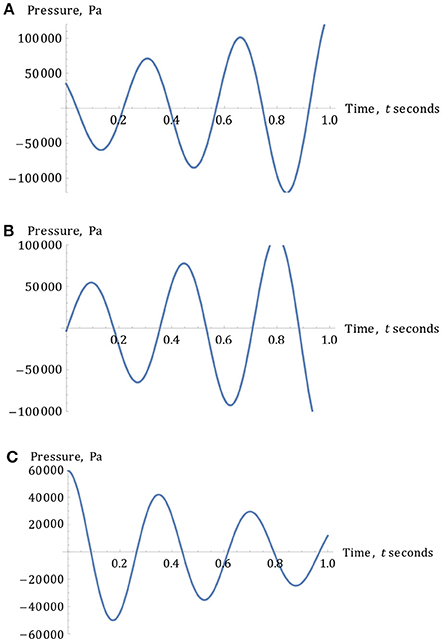
Figure 14. (A) The variation of wave-pressure vs. time for any pressure magnitude and for any positive- or negative-valued shear wave-velocity, c. Therefore, the solution blows-up given , as t → ∞, where is both fixed and finite, and is eventually exceeded by the increasing temporal-variable, t. In this diagram, a wave-velocity of c = 4 m/s was adopted to highlight the phase-shift more clearly. Note the apparent existence of an under-pressure between the occurrence of the phase and the time t = 0.2 s. (B) The variation of wave-pressure vs. time for any pressure magnitude and for any positive- or negative-valued larger shear wave-velocity of c was adopted. Therefore, the solution blows-up given , as t → ∞, where is both fixed and finite, eventually exceeded by this increasing temporal-variable, t. In the plotting of this diagram, the wave-velocity of c = 40 m/s was used. (C) A solution curve for the variable pressure: , where x is fixed at 0.176 m, s, m, c = 4 m/s, , and α = 54, 500 Pa, each scaled appropriately to yield a maximum test pressure at s of 50,000 Pa. Graphs for any values of the shear wave-velocity c are similar, as before, although for higher values than 4 m/s the phase approaches the origin more closely and rapidly. Note the initial under-pressure in this solution-curve.
Nature of Initial-Boundary-Conditions Ultimately Determining Type of Damped Pressure Observed During Experimental Shock-Tube Observations
At the beginning of the section Approximate, Smoother and More Continuous Forms of the Friedlander Curve to model Pressure Versus Time from Initial-Boundary-Conditions and thereafter, a solution of the problem via the method of characteristics illustrates that the nature of either observed, or chosen, initial conditions dictates the type of damped pressure observed, particularly as witnessed during experimental shock-tube simulations.
Commencing with the solution of the separable ordinary differential Equations (85) and (86), in which the second, alternative, initial spatial condition is taken to be m [5], with , the generalized unknown quasi-constant, k, yields Equation (98), which may be written:
In the analysis describing the experimental observations, the pressure, u(t, x), was often seen to increase to a local peak-maximum at the point where m and then to decay to zero, possibly whilst oscillating.
Since Equation (102) is often positive (as in the section Pressure-Time Solution-Curves for Different Maximum Pressures and Boundary Conditions Closely Resembling the Friedlander Curve), from the point at which the phase first occurs, up to the maximum peak and negatively damped thereafter, as shown in Figures 10A,B, the most appropriate boundary condition one should use is either of the Equations (51) or (52). At least one of these boundary conditions yields a particular-solution suitably matching experimentally observed data, as the graphical plots illustrate. Since either of these boundary conditions involves an exponential term, ultimately decaying over increasing time after the occurrence of the peak, due solely to the negatively increasing indicial exponent, both are more appropriate for that part of the model where a positively damped exponential term is ultimately increasing indefinitely. This yields to the conclusion that either of the boundary conditions, Equations (51) or (52), lead to the correct usage of Equations (102) and (103) in the form of:
and:
each suggesting that they describe the observed physics.
When, however, the same initial conditions are reversed, such that s, [6], and, again, , we similarly obtain the two previous equations, Equations (100) and (101), for the purposes of considering the time-phases alone.
We may write:
and:
Here, one may observe that the solution-curves blow-up as t → ∞ and are not ideal, long term, for the purposes of plotting the pressure for the above model, given previously mentioned conservation issues.
However, unless an experimentally observed pressure increase needs modeling, again to plot eventually decreasing pressure variation as before, Equations (99) and (100) can be modified to plot the solutions of u(t, x) vs. t if the boundary conditions:
and:
are adopted, in which the indicial part of the exponential function in each of the above is positive. This means that, when Equation (95) is substituted into the above, the particular-solutions can be re-written as:
and:
To model either of these latter equations depends on which is more physically appropriate. It is noticeable that, as time increases, the analysis indicates the indicial part of each exponential becoming negative—and hence a decreasing pressure—once more, for fixed x as t → ∞, as shown in Figure 14C, above.
Hopf-Cole Transformation in Obtaining Heat-Diffusion Equation From Burgers' Equation to Model Shock-Wave Energies
The next step is to supplement existing theory of observational results by predicting the neurological shock- and pressure- wave energies that may eventually be detected following the exposure of military personnel to IEDs. According to Risling [9], pressure-wave energies are very difficult to measure. Considering this, one should at least be able to theoretically predict their magnitudes prior to any discovery not yet cited in any existing academic literature. To calculate the energies of a resulting shock- and pressure-wave system, we need to use the Heat-Diffusion equation. Since these energies are directly related to the initial impact, we need to illustrate the validity of using the Heat-Diffusion equation, which turns out to be closely linked to Burgers' equation for the shock-wave solution. This is achieved by solving Burgers' equation via another method, utilizing the Hopf-Cole Transformation.
Commencing once again with Equations (15) or (16), representing the wave-propagation of a shock- and pressure-wave, we have:
in which the energy-profiles are similarly non-linear. We put:
such that ut = ψxt, ux = ψxx and uxx = ψxxx. Then, substituting each of these derivatives into either Equations (15) or (16) yields the respective PDE, as shown below in Equation (124):
This transformed Burgers' equation can now be written in its alternative form:
or otherwise:
Eliminating the partial derivatives, we obtain:
Now, let:
such that:
and:
Each of the above was obtained using normal differential rules of calculus and elementary algebra. Substituting each of these differential expressions into Equation (108), we obtain:
or:
leading to:
Simplifying Equation (134) by canceling the factors of −2γ and ϕ on each side, we obtain the final Heat-Diffusion equation:
in which γ now represents the thermal-diffusivity coefficient, 1.38 × 10⁻⁷m2/s. In fact, the sum of both this and the mass diffusivity term of 1 × 10⁻⁹m2/s, namely 1.381 × 10⁻⁷m2/s, barely differs from the former and, it appears that in transitioning from the solution for Burgers' equation to the Heat-Diffusion equation, there has somehow been a branching off (or bifurcation) of the brain's original mass-diffusivity value to that of its own thermal-diffusivity, as characterized in the latter. This has been achieved via the simple but celebrated Hopf-Cole Transformation that appears to have potential similarities with the Hopf-Cole Bifurcation process.
Conservation of Energy and Calculation of Total Energy Within Each System
Given the validity of conservation laws, we show that the total energy, ET, of any system is constant, prior to commencing the derivation of the necessary momentum- and energy-distributions and their respective values.
Henceforth, the above Heat-Diffusion Equation, (135), can be written in two forms:
or:
Since the difference between the two sides of Equation (136), and therefore Equation (137), is zero, we may write:
or, more explicitly:
where C is a constant.
Hence, dividing both sides by γ, for convenience, and then integrating the RHS by parts over the range L ≤ x ≤ R, with a more general variable, k, yields:
or, multiplying by γdk again, and integrating, we may write:
where K1 is also constant.
Although Equation (141) indeed represents a constant of integration, it is actually a function of k, namely the evolutionary (and spatially-based) function, E(k), since it has been integrated with respect to the independent variable, as can be seen in Equation (140). We can therefore assert that the total energy is constant (for the resulting Heat-Diffusion equation), E(t, x) = E(k) = K1, hence the whole system is conservative.
Similarly, multiplying each side of Equation (135) by ϕ and then integrating, we have:
Since the functional time-evolution of ϕ(k), over the given spatial-range is known to be:
then Equation (145) can be written:
It turns out that the above integral, Equation (145), in tandem with Equation (138), can be written more simply as:
where K2 is constant.
As explained by Olver [10], by simply integrating Equation (135) with respect to dx, between any two, given, spatial limits, x = L and x = R, in combination with Equation (137), one can similarly show that ϕ(k) is equal to a constant value. In the case of the sections Burgers Equation Derivation in Terms of Velocity and Pressure—Simplified Result of Navier-Stokes Equation and Boundary Conditions Within a Typical Case, a general variate, k, has been introduced, prior to considering phase-shifts and the factor ct, such that, at t = 0, we have:
Equation (147), like Equation (145), represents both the total sum and the time-evolution of this quantity over the spatial interval L ≤ x ≤ R, where L = 0 and R = 0.176 m. Thus, we may write:
or, more succinctly:
which is identical to Equation (147), and where K1 represents the steady-state equilibrium of the solution, ϕ(k), as t → ∞, therefore satisfying the strong maximum principle:
The above principle may also be applied to the spectral distribution of energies, E(ω):
again, in which the energy-conservation of the system, is evident.
Equation (150) also yields the maximum Energy, E(ξ) = E(0, x) = E(0, ξ) Joules, at the spatial coordinate, x = ξ when time t = 0 s. This mathematical statement can be explained more literally in terms that, as t → ∞, the dynamic energy-profile of E(k), never yields a greater magnitude, at any spatial-point, x, nor at any time, t, than the initial maximum value, E(ξ). This latter point is a strong factor associated with the total finite energy of the system, in keeping with conservation laws. If total energy were to be calculated to be greater, or even infinite, in magnitude, than E(ξ), then the law dictating that energy must be conserved would be violated.
From Equation (123), ψx = u(t, x) can be re-written in terms of k, such that ψk(k) = u(0, x) = u(k). Thus:
particularly when the time is initially zero. Hence, substituting Equation (128), ψ(k) = −2γ ln (ϕ), into Equation (151):
and, after further algebraic manipulation:
or, more simply:
By re-substituting k = x − 2.325 × 10⁻³, and by applying integration-by-parts of the exponent, , between the given limits of L = 0 and R = 0.176 m, and where α represents maximum pressure, with , as in the sections Burgers Equation Derivation in Terms of Velocity and Pressure—Simplified Result of Navier-Stokes Equation and Boundary Conditions Within a Typical Case, we find:
where k = x − ct − 2.325 × 10⁻³ + 4.65 × 10⁻⁴c. Whether x = 0 at t = 0, or x = 2.325 × 10⁻³ m at t = 4.65 × 10⁻⁴ s, the scaling makes no difference to the analysis, nor to any of the values obtained.
Integrating Equation (156) by parts, we obtain:
At the point where x = 2.325 × 10⁻³ m and t = 4.65 × 10⁻⁴ s, where we take a maximum test-pressure of 50,000 Pa to occur, it transpires that Equation (157) yields a zero result. So, by correctly adopting the original boundary condition, in the case of the sections Burgers Equation Derivation in Terms of Velocity and Pressure—Simplified Result of Navier-Stokes Equation, we obtain the maximum magnitude of the right-hand-side of Equation (156), namely Joules, which bears the same value irrespective of the shear-wave velocity of c m/s. Substituting the usual values into the constant coefficient part of Equation (157), this equates to:
The right-hand-side of Equation (157) can now be substituted into the energy-evolution Equation (154):
but, since the analytic solution to this latter equation, Equation (159), is very complex to obtain, only the graph of Equation (157) has been plotted in Figure 15 below. As an illustration, the graphical plot of Equation (157), Figure 15, displays damped periodic behavior, thus rapidly approaching the very large limiting value of 3.1 × 10¹⁰ Joules.
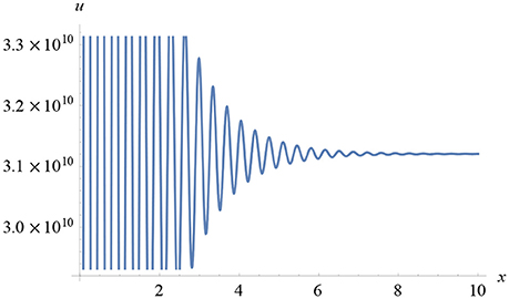
Figure 15. Plot of u(x) vs. x illustrating the function's tendency to approach the limiting value of approximately 3.1 × 10¹⁰ Pascals, assuming that there is no loss, nor transfer, of energy into or out of the system, according to the adiabatic law.
Having established the long-term behavior of Equation (157), which ultimately approaches a constant value, it is possible to predict the behavior of the long-term energy profile. The energy, defined by Equation (159), when integrated itself between any spatial limits, ultimately yields a value approaching a constant total energy magnitude with increasing time and space, seen in Figure 15 below. This is because the exponent in Equation (159) has a negative limiting value, meaning the exponential of this parameter results in a constant result for the long-term energy itself.
The above statement is consistent with knowledge of shock-wave energies, in which all energy profiles drop, usually rapidly, to zero, or at least to negligible values with increasing time.
Thus, the plot in Figure 15 yields a maximum peak value of 5.74 × 10¹⁰ Joules when x = 0 m at t = 4.65 × 10⁻⁴ s, with a rapidly decreasing profile that approaches the limit of around 3.1 × 10¹⁰ Joules at x = 0.176 m, when using γ = 1.39 × 10⁻⁷m2/s. Since the long-term behavior of the energy is calculated from the equation:
on substituting the value ∫ u(x)dx = 3.1 × 10¹⁰ into the above, we find that:
So the above factor, in which E(t) ≅ 0, not only suggests that the long term energy certainly dissipates to a negligible quantity, it also reinforces the principle of conservation of energy, in this case stating that the total energy, ETotal, never exceeds the maximum energy of the whole system, such that ETotal ≤ E(ξ), or alternatively depicted by ETotal ≤ EMax.
Criticisms and Potential Problems With the Model in the Section on Conservation of Energy and the Calculation of Total Energy of Each System
In the section Hopf-Cole Transformation in obtaining Heat-Diffusion Equation from Burgers' Equation to model Shock-Wave Energies, the analysis suggests that Equation (135), using the original boundary condition, u(k) = αe−k sin (ωk) dk, therefore results in a total energy of magnitude, ET, which is consistent with energy conservation laws. However, the solutions from this point onwards often tend to indicate that Dirac-delta based Gaussian functions—such as the Normal distribution—become important factors in understanding the nature and behavior of energy transfers. Just how relevant these are to IED-blast wave mechanics in the human brain remains to be seen, due to the conservation laws and the finite nature of energy. If they are relevant, then it is conceivable that a modified Gaussian approach will be more appropriate.
Application of Fourier Transform to Uniform Distribution (Boxcar Function) to Obtain Gaussian-Based Sinc (ω) Function
In this section, application of the Fourier Transform to the Uniform Distribution (Boxcar Function) will be discussed. This application of the given integrals will result in the obtaining of the Gaussian-based sinc (ω) momentum-space function.
As Olver [10] suggests, the approach required to deduce a more appropriate model would develop an equation involving a characteristic variable k, perhaps in the form of a variable quotient. For example, using Fourier Analysis, one can deduce:
in which ξ represents one's choice of spatial limits, or spatial-phase values, along the x-axis.
In the section Determination of the Value of the Constants of Proportionality, α and β, and Maximum Pressure, PM, the characteristic variable in Equation (75), for example, can be written:
Since the energy, as described in the last two sections, is largely concentrated at a single point, from which its evolution with respect to time often very rapidly decays in accordance with the conservation laws, it is necessary to consider this factor in the following section, modeling this dynamic process as accurately as possible.
A Concentrated Point-Source of Energy, E(t), Rapidly Dissipating With Increasing Time
For the purposes of a straightforward example, we commence the analysis by considering the general profile of a uniform distribution, or boxcar function, [10], as:
where we choose a constant, c, to simply represent the constant height of the rectangular distribution over the given spatial-limits, . In Equation (164), if we assume that the transformed expression shows the maximum energy of the whole system (under the subsequent curve that is produced), f(x − ξ) = E(x − ξ), to be equal to c at the spatial-phase of x = ξ, then it indicates that the value of E, as measured at any other point in space or time, cannot be greater than E(ξ) at any other given point for x ≠ ξ. The argument is identical at x = ξ = 0, such that E(x − ξ) = E(ξ) = E(0) = c, and it is again asserted that E(x − ξ) = 0 when x ≠ ξ. All this implies that the dynamic, energy-based, evolutionary system approximates the Dirac-delta function:
whose integral is simply the likelihood of identifying “a particle,” or at least the maximum energy, E, at x = ξ. It should be noted here that, normally, the transformation of f(x − ξ) into a function of frequency, for example, such as F(ω), is usually taken to represent the momentum space. Certainly, for these models, it turns out that F(ω) is closely linked to the energy, E(ω), by way of the spatio-temporal variables, x and t, with E(ω) being linked to F(ω), because of the areas under the produced curves and, more appropriately, dynamically represented as a function of time, or E(t). The units and dimensions of the area under each curve are those of ML2T−1, or the momentum multiplied by the distance an object travels.
The general Dirac-delta function states:
or:
The main reason why the Boxcar function above, the Dirac-delta function in the definition below, and thereafter the Fourier Transform, are discussed with this level of detail, is because each will occur in the conversion of the initial signal into the energy contained within the system as a whole.
Definition 2: The Dirac-Delta Function
Since, from Equation (165), the Dirac-delta function states:
where the total area (or probability) under its curve generally needs to be equal to unity, we must consider a normalized sample between the limits of so that, when ω = 2πx and , Equation (165) equates to 1, for any generalized function, f(x). By substituting in the given limits and angular variables, we have:
If the function at a given point in space, ξ, for example, is of a maximum value, such as Fξ(ω) = FMax, then:
Here, ω has been used, rather than ξ, since the evolutionary nature of the potential function, Fξ (ω), is more conveniently measured in terms of angular-frequency (or just frequency), and only has a value at the spatial coordinate, x = ω = 2πk.
For the dynamically dissipating, limiting value of the momentum-space profile, F(ω), with f(x) = e−ikx, we first determine the correct exponential form of F(ω), via the Dirac-delta function in Equation (166) above. Thus, setting the whole area of the curve, δ(x − ξ) to 1 square meter, and , the Dirac-delta function states:
Given that, for an ordinary exponentially decaying curve, f(x) = e−iωx = e−i2πkx, where dω = 2π dk, then we set k = x − ξ, such that dx = dv. Hence, Equation (167) can be written:
Since , we find:
or:
Since we know that the given system only approximates to the Dirac-delta function, such as when we arrive at the sinc(ω) function from the Boxcar function as ω → ∞, we can assume that the actual momentum-space, F, peaks at a maximum value, FM, rapidly dissipating to a lower limit, usually zero, as described by an exponentially decaying function. Based on this latter postulate, on integrating Equation (167) again, we obtain:
and by applying the relevant boundary conditions, f(ξ) = e−2iωξ at t = 0 when x = ξ, we have the following exponentially decaying profile:
or:
To convert the boxcar function into a more meaningful distribution (namely the sinc (ω) function), we apply the Fourier Transform, converting the function, u(x), into its respective momentum-space-distribution defined by:
where and ω represents the angular-frequency of the representative momentum-space and energy-spectrum. Since u(x) = α(x − ξ1) − β(x − ξ2) = c, we can substitute this latter result into Equation (178). Thus:
which, using elementary mathematics, integrates to:
or, more simply:
In this latter result of Equation (182) if, for example, and , preserving reflective symmetry with a resulting range of 1, we have:
which is written:
or otherwise defined by:
Here, the momentum, F(ω), is a function of angular-frequency (or distributed with respect to the angular-frequency), ω, which represents certain levels of excitation. This is a significant result, explaining the nature of the Dirac-delta function within the remit of Quantum Mechanics, as briefly discussed above.
What the above function tells us, especially through a graphical plot, is that as ω → 0 (for increasingly higher frequencies), then . However, when ω begins to increase, so that the energy wavelengths, λ, become infinitesimally small (or λ → 0), the science is explained by the quantum theory inherent in what is now a probability distribution, assigning a degree of probability to the position of a sub-atomic particle at time t.
It is a fundamentally quantum mechanical concept that when the frequency, defined by , of an energy- or momentum-space sinc-distributed-energy function becomes ever increasingly larger, even as it approaches infinity, ω → ∞, sinc (ωx) becomes ever thinner and taller in width and height, respectively. It eventually becomes infinitesimally thin and infinitely tall, and for every reduction in wavelength, the sinc (ω) function enlarges by a factor of λ, such that:
where .
As demonstrated by algebraic manipulation, this creates a Gaussian-distribution approaching the Dirac-delta function, approximating the nature of many quantum mechanical effects. This would include energy-distributions and momentum-spaces, for example, witnessed within these areas of physics, mathematics and science—and also within many associated scenarios.
However, there is another Gaussian function perhaps more appropriate for illustrating energy distributions. This distribution is defined by the boundary condition for the momentum-space alone, namely:
or, more generally:
which requires that the distribution of u(t, x) must be square integrable, such that the distribution of u(t, x) over a smaller sample of an infinite range can, according to Olver [10], be written in generalized coordinates as:
with
each of which obeys the conservation of energy, [10, 11], and still preserves the resulting normalized-distribution.
Equation (190) may also be shown by multiplying Burgers' equation, in Equation (17), by u(t, x), and then applying integrals, to obtain the energy conservation law, [10, 11]:
Within many physical contexts such as this one, and as highlighted by Green's Theorem, the right-hand-side of Equation (192) represents the scalar magnitude of the energy, E, equal to the flux—the rate of flow of the energy per unit area having the solution:
hence the result in Equation (190).
If one substitutes Equation (188) into Equation (191) and then proceeds to apply the error function to the resulting integral, one obtains the scaling factor, in this case, equal to:
Thus, a function such as:
will return the more general scaling factor or function of the form:
where a is a parameter assuming either a constant value, or the form of a variable, such as t or x, dictating the nature of the resulting energy-space and the latter's respective individual values.
To obtain the energy-space resulting from the sinc (ω) function in Equation (185), one needs to find the integral of its square, namely:
so that:
or, more simply:
where FMax is the maximum value of the integrated function.
Heat Equation Modeling the Brain's Existing Natural Temperature Variation
In the section Hopf-Cole Transformation in obtaining Heat-Diffusion Equation from Burgers' Equation to model Shock-Wave Energies, the Heat-Diffusion equation, Equation (134), was expressed in terms of ϕ(t, x), which itself is some function of u(t, x), thus linking the two. The solution to Burgers equation, in terms of each of these variables, will be achieved at a later stage but, for now, we re-state the Heat-Diffusion equation for a constant, existing, initial temperature, u0, in the absence of any external energy input. This permits thermal energy to be naturally transferred from regions of high to low potential, as will occur for the human brain undergoing many complex influences. This relationship is more simply written as:
where the same functional notation, u(t, x), is now assumed to describe the transfer of energy in the human brain, resulting in an increase in its thermal energy. Here, γ represents the heat-diffusion coefficient equal to 1.39 × 10⁻⁷m2/s, verified from data given by Elwassif et al. [12].
We should consider that, unlike the energy defined by Burgers' equation in Equation (190), the Heat-Diffusion equation yields the total energy, for zero initial temperature, of the system as:
where ρ is the density of the brain, taken to be a constant overall value of 1,040 kg/m3, and cp represents the brain's specific heat capacity of 3,650 Jkg−1C−1.
The complexity of this situation requires some assumptions, based on pressure profiles in earlier sections. To facilitate a simpler solution, we first solve the Heat-Diffusion equation for an un-forced system (in the absence of an IED-blast) where the temperature decays to zero:
and then reintroduce the constant heat source, u0 ≠ 0, into the final, time-independent, steady state solution:
A further assumption can be made that, at t = ϵ > 0, there is zero energy flux due to the absence of an IED-blast and, therefore, a zero-energy pulse until the point where x = ξ > 0, the latter being the point of any shock-wave impact immediately after a blast.
At x = 0 when t = 0, we may adopt both Dirichlet and Neumann boundary conditions, u(t, 0) = u0, u(t, L) = u0, u(0, x) = u(x) = ϕ(x) and ux(t, 0) = ux(t, L) = 0, so that periodic boundary conditions enable the solution to be satisfied at the given limits, and where the brain's own natural heat-source, u0, represents the normal temperature or energy of the human brain at both x = 0 and t = 0. Given the absence of any IED-energy pulse, in adopting the Heat-Diffusion equation, we may assume that the temperature profile will oscillate about the brain's natural temperature, [12–17], to some extent so that, under normal circumstances C (or 310.15 Kelvin) as t → ∞.
We commence by modeling the behavior of the solution over the range stipulated by 0 ≤ x ≤ L, with L = 0.176 m, whereby we consider a narrow “bar-like column” through the brain [18], except with different boundary conditions that will be considered at a later stage.
Using the following eigen-function substitution for an exponentially decaying sinusoidal temperature profile to solve Equation (202), we have:
where λ > 0. Putting γω2 = λ and partially differentiating Equation (204) for ut and uxx, we obtain the equivalent eigen-functions, otherwise illustrating a summation of ordinary differential equations (ODEs), denoted as:
and:
Substituting Equations (205) and (206) into Equation (202) the following ordinary differential equation (ODE) is obtained:
On re-substituting λ = γω2, canceling the common summation signs and other factors on both sides and separating the variables, we obtain the second order, simple-harmonic-motion, ODE:
to which the solution is:
where, from Equation (202), ϕn(x) = u(x) at t = 0.
Since this is a thermal energy or temperature-based problem, rather than one based solely on the flux-based profile, we need to use both Dirichlet and Neumann Boundary Conditions, which assume that at x = 0 and x = L, u(t, 0) = u(t, L) = u0 = 37 and .
Given that u(t, 0) = u(t, L) = 37, then the second partial derivative of Equation (208), which is the derivative of Equation (203), is:
The basic steady-state temperature solution is the analogy to Equation (209), and can be obtained after reversing the process, re-integrating Equation (210), twice, and solving simultaneously with Equation (209), the solution being:
where A and B are constants of integration.
Substituting both sets of initial conditions into Equations (209) and (211) at x = 0 and x = L = 0.176 m indicates that A = 0 and C. Thus:
where, from Equation (204), we see that ϕ0(x) = b0 = u0 is another solution.
By substituting Equation (212) into Equation (204), we may write:
which is the sinusoidal temperature profile for zero initial temperature (C when x = 0 at t = 0).
This complementary solution may now be added to u0 to obtain the general steady-state solution, again indicated by Equation (203). This amounts to shifting Equation (213) along the vertical axis of its graph by C units to produce the steady-state temperature profile for the human brain about this temperature, given by the more general series of n solutions:
By letting , and , Fourier Analysis tells us there are any number of such eigen-solutions as follows:
where u0 is the equilibrium, average, long-term temperature (of 37°C), about which it varies, slightly, over time, and where the sequence of terms containing cn, for n = 1, 2, 3, …, are the Fourier coefficients [10].
Assuming the limit of a discrete sequence of the form of Equation (215) approaches the steady-state solution of u0, with t set equal to a constant, ϵ, it can be shown that since:
after finding the first Fourier coefficient, c1, using the formula:
we obtain:
where we have:
and, by applying the Riemann sum [10], Equation (218) can be expanded and integrated, namely via the Riemann integral, initially as a first closed form approximation for the above series in the form of:
where we have set a = γϵ, , and , from Olver [10], p. 265, 2014.
However, since Equation (219) yields absurdly high Dirac-delta type values (which requires application of the Fourier Transform), it is therefore inappropriate for modeling the variation of the normally existing brain temperature in this specific case. To overcome this issue, we can instead write Equation (218) as a Riemann integral in terms of the spatial variablex, namely:
for the range −0.088 < x < 0.088, where in the limit.
This yields a more reasonable range for the temperature distribution than the series represented by Equation (219). It also smooths out the otherwise much higher temperature values (including the peak value) of Equation (218), which is the un-transformed solution briefly discussed below, whilst simultaneously illustrating the naturally varying sinusoidal profile. Within this context, the conversion of each summand within the original series in Equation (218) to either a definite or an indefinite integral in Equation (220) serves to sum over all eventualities within the convergent limit. This produces a more accurate result for a brain that has not yet been subject to an IED-blast.
The temperature profile, as expressed by Equation (200) and its solution for the given parameters in the section Calculation of the Brain's Existing Natural Temperature Variation below, in producing each of the snapshots-in-time displayed by Figures 16A–G, indicates the presence of slight instabilities in the existing brain temperature even in the absence of other external influences.
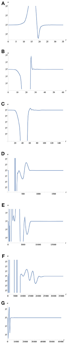
Figure 16. (A) Heat-Solution up to 35 s. (B) Heat-Solution up to 60 s. (C) Heat-Solution up to 160 s. (D) Heat-Solution up to 30 min. (E) Heat-Solution up to 5 h. (F) Heat-Solution up to 11 h. (G) Heat-Solution up to 16 h.
In Figure 16B, there is a sharp increase (but only by a fraction of a degree), then a sharp decrease in temperature between 10 and 20 s, before rising again and approaching the equilibrium temperature. Figures 16C–G continue to outline this increase and decrease in energy and temperature even further, along with the behavior of each profile oscillating to an even greater extent as time approaches the 11 h stage in Figure 16G.
Although this profile appears to finally approach the equilibrium temperature of 37°C at approximately the 13 h stage in Figure 16G, because of the nature of the mathematically convergent sequence that forms it, one may assume that these temperature oscillations will always continue to occur indefinitely due to the sinusoidal term in Equation (218) and other biological influences such as the existing heat-source of the brain.
Calculation of the Brain's Existing Natural Temperature Variation
The calculation of possible naturally existing energies and temperatures within the brain now follows. From Equation (211), we know that at x = 0 when t = 0, then u(x) = u0, such that E0 = ρcpu0. Therefore, since the total energy is obtained from Equation (201), we have:
but only in situations when the initial internal temperature and energy, u0 and E0, are themselves zero.
However, we know that the initial energy is not zero, due to existing brain temperature, so we may rewrite the above energy integral, Equation (201), as:
so:
where if, as stated, E0 = ρcpu0 is a non-zero constant at the point x = 0 when t = 0, we may write Equation (221) as:
By rearranging the above equation, a steady-state solution for the energy is:
where ρcpu0 is initially independent of both time and space, and is neither a function, nor a multiple, of either.
To determine the maximum temperature of the system, we need a time, t, as close to zero as possible at which the maximum value of the curve takes place. The scaled characteristic diffusion time is therefore , where we see that s, this latter quantity being the peak-time approximation at this point. Because there is a rapid convergence of the sine terms toward the equilibrium value of 37°C, in Equation (218), around which it oscillates indefinitely, the leading term for n = 1 of this sequence is normally sufficient to calculate the resulting maximum temperature. We therefore note that, by re-scaling this time-dimension as and substituting L = 0.176 m and γ = 1.38 × 10⁻⁷ m2/s, we find that t* = 6.31 h, which is roughly the time taken for this system to (ideally) settle down to equilibrium again. Putting n = 1 and for the maximum temperature obtained at the “center of the column through the brain,” Equation (218) yields a value of:
which returns the rather unlikely value of 54.33°C. Clearly, this is too large a value for standard variation in a normally heated and resting brain, whose equilibrium temperature is 37°C in the absence of any other external stimuli. Therefore, we now adopt Equation (220) to see if it is possible to profile a more realistic energy and temperature solution.
Substituting Equation (220) into Equation (224), we obtain:
and, since the characteristic diffusion time is , we have:
On integration of Equation (227), we have:
Since Equation (228) has been obtained via the Riemann integral, where the mid-point is for the range 0 ≤ x ≤ L, then, with n = 1, the solution yields a maximum energy of 1.406 × 10⁸ J and a temperature of 37.055°C. This latter figure appears reasonably consistent with observed temperature fluctuations for a normal and un-inflicted human brain in its resting state [19]. The sinusoidal temperature profile of this is illustrated in Figure 17A.
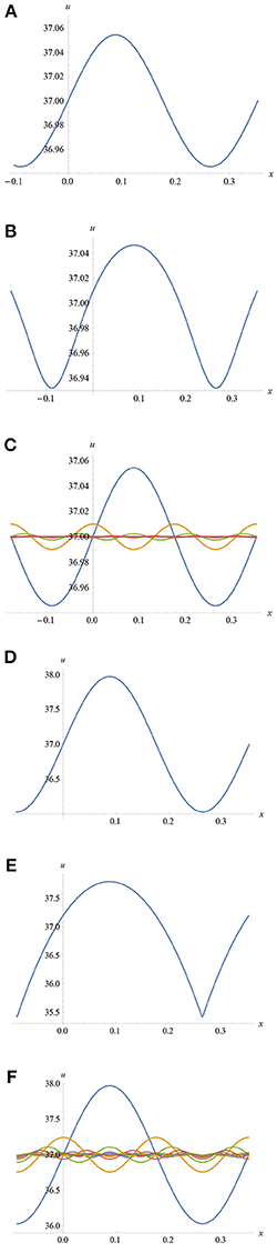
Figure 17. (A) Variation of Temperature Distribution obtained from Equation (228) for n = 1. (B) Temperature Variation as a result of adding the series defined by Equation (228) for n = 1 to 50. (C) Individual Temperature Profiles for n = 1, 2, 3,…, generated by Equation (228). (D) Variation of Temperature Distribution obtained from Equation (229) for n = 1. (E) Temperature Variation as a result of adding the series defined by Equation (229) for n = 1 to 50. (F) Individual Temperature Profiles for n = 1, 2, 3,…, generated by Equation (229).
In Figure 17A, the temperature does not exceed the peak value, but gradually smooths out from the mid-point onwards as it “decays” with time, consistent with energy conservation. Given that the temperature ranges between a minimum of 36.95°C and a maximum of 37.054°C over a normal period of life, it is clear to see that for n = 1, 2, 3, ..., k each of these values must oscillate, as the sinusoidal term suggests, although it is the tendency of the system to approach the steady state equilibrium temperature of 37°C. Figures 17B,C illustrate both the sum of all the individual temperature profiles in Equation (228) for n = 1 to 50, and the individual temperature distributions, respectively.
It is also of importance to mention, here, that if Equation (218) is integrated term by term (but leaving the first term, u0, alone), in the form of [10], where , then we obtain:
Substituting in the same values as before for each of the parameters in Equation (229), with n = 1 and , the first term returns maximum and minimum peak-values of 37.97°C and 36.03°C, respectively, whilst the sum of all the Fourier terms up to n = 50 yields 37.8°C and 35.04°C. The graphs for each case can be seen in Figures 17D–F, below.
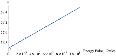
Figure 18. Graph of variation of temperature vs IED-blast energy.
Calculation of Induced Temperature Variation and Energies Within the Brain Due to an IED-Blast
In the event of an IED-blast, energy is transferred to the human brain within the vicinity of the explosion and added to the brain's existing heat energy, u0, this being likely to make more of a difference to its temperature variation.
We now consider an additional cylindrical explosive blast forcing term [18, 20], of , which we may assume, after this energy has entered the brain, decays exponentially in the form of . It has been assumed, here, that the full amount of IED-energy, EP, initially enters the brain, whereby it is more likely that only a fraction of this does so in reality. Much of this depends on the number of military personnel present, along with the presence of other physical obstacles (and the nature of the terrain), greater numbers of which tend to absorb a lower quantity of energy per person or object in such circumstances [18]. This means that any energy transfers and temperature increases are more likely to be less pronounced and intense when factors like these are considered.
Here, the velocity, v, of the blast is normally taken to be a constant, and where m/C is the ratio of the mass, m, of the cylindrical metal casing to the mass, C, of the explosive material. This situation may be quite different for a spherically designed thermo-nuclear device, for example. Thus, we may attempt to solve the modified, forced, Heat-Diffusion equation, to test if this is an appropriate model. The forced equation may therefore be written as:
with u (0, x) = 37, and where is the variable energy density emitted by the IED blast-wave as it impacts the skull. Again, we substitute u(t, x) = ∑ϕn(t) sin nωx, with the energy density , into Equation (230), without assuming that this energy decays according to the same exponential parameters as elsewhere, although it may well do so. We therefore find that and , such that the Heat-Diffusion equation now becomes:
which simplifies to:
where for convenience, and where EP is taken to be constant. To solve this problem, we need to find the Fourier sine series of the term, , on the right-hand-side, so, keeping all variables in terms of the temperature, we have:
We obtain the bn by performing the integral:
such that:
resulting in:
or:
Now, for even n = 2, 4, 6, ….,
and for odd n = 1, 3, 5, ….
Equation (232) can be equated to:
for even n = 2, 4, 6, …, and:
for odd n = 1, 3, 5, ….
Equation (241) can be solved to yield the complementary function:
where cn is a series of constants, each yet to be determined.
Now, the solution to Equation (242) is obtained by using undetermined coefficients, which is perhaps more straightforward here than using the integrating factor method. Thus setting , we find that . Hence, Equation (242) can be written:
where we find:
Substituting this value into , we find one solution:
Henceforth, by adding this solution, ϕn, to Equation (243), we have the general solution:
Since the eigen-function for the solution yields , on substituting this into Equation (247), we have:
The Fourier transform of the various cn is obtained by first computing the Fourier series for the initial condition (att = 0):
yielding:
hence:
or, after substituting Equation (251) back into Equation (249), we obtain:
Equating this last result with Equation (248) at t = 0, dropping the summands and canceling common terms, yields:
which leads to:
This means that Equation (248) can now be re-written:
Before we write down a full thermal solution for u(t, x), it is important to note that there is a unique thermal equilibrium solution, as indicated in the section The Heat Equation Modeling the Brain's Existing Natural Temperature Variation, of u0 > 0:
where:
as time increases indefinitely, t → ∞.
Henceforth, a full temperature solution is:
Once again, substituting , , and , assuming convergence and applying the Riemann sum, this energy-temperature solution (per unit mass in kilograms) can be written as the Fourier Transforms for both the frequency and spatial domains:
respectively.
The energy profiles are simply expressed as:
Since we have already defined: and using data provided by Jacobs [20], and others such as Gerber [21], if we take v = 1,732, 2,500, 3,162 and 4,000 m/s (as based on the referenced literature) and , then the initial IED-blast energies, for a value of , are calculated as:
Integrating Equation (260) with respect to ω on the interval , and substituting the above (and additional) energies into the solution, with an initial scaled peak-value of, yields several linearly increasing maximum, “peak,” temperatures (at x = 0.088 m). Some of these are displayed in Table 1. Figure 18 also shows the apparent linear relationship between these energy pulses and the possible temperatures resulting from the solution to Equation (260).
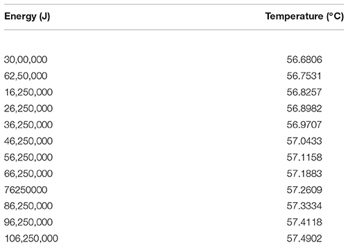
Table 1. Table of temperature values vs IED-blast energies.
Significantly increasing the size of the initial energy pulse within this model results in only fractional linear temperature increases (between 56.68°C and 57.49°C) over just less than a 1°C range. Each of these temperatures corresponds to the range of pulses between 3 × 10⁶ J and 1.0625 × 10⁸ J, although the difference between them and the steady-state value of 37°C is significant at a maximum total temperature increase of 23°C for this given energy range.
Additionally, this also means that the maximum peak energy entering the brain is itself raised from around 1.40452 × 10⁸ J to as much as 2.3 × 10⁸ J for the energy range illustrated in Table 1. No matter how much energy is imparted to the system by a cylindrical blast (which arguably results in a Dirac-delta spike, whose maximum peak continually increases with increasing energy input), the temperature will increase only fractionally beyond what is calculated for the first pulse—although the theory suggests that one may linearly extrapolate larger temperatures corresponding to even larger energy-pulses. However, one should observe that these calculated peak energy values do not necessarily represent energy-densities, as the latter refers to the area under each respective curve and, henceforth, each quantity of energy contained within the brain as a whole for each energy pulse.
Just how large an energy pulse needs to be to violate this pattern of linearity remains to be seen; for example, whether an explosive device is cylindrical or spherical—such as a nuclear explosion in the latter case—will have differing effects on the body and brain. It is possible that some of the energies in Table 1 beyond the 16 MJ blast are more indicative of a thermonuclear energy emission, in which case a different function for the energy-pulse would need to be adopted and substituted into Equation (260). As was alluded to above, and to be explained more fully later, when these Gaussian curves get taller, their widths also decrease proportionately so that the same area under them—representing the energy density contained with the brain post-blast—is also maintained. For such a situation, and others like it, the temperature—or energy density—is a constant [10].
Using the same energy values in Equation (261), again, if we vary the constant k, and set it equal to ω2, such that , we find that the maximum energy values are only hundredths of a degree lower, and change very little overall.
Also, it appears that by considering many Fourier terms in either the integrated Fourier series or Equation (260), the square of the original value of angular-frequency of the initial energy pulse, after entering the brain, makes very little further difference to any temperature increases within the brain due to the increasingly vanishing nature of the exponential term in the second integrand.
Within this model, it appears that the parameters and structure of the human brain, such as the diffusivity constant, γ = 1.38 × 10⁻⁷m2/s, as well as the nature of IED-blast energy emissions and transfer, are implicit in the Heat-Diffusion equation within this context. Many of the other, as-yet, unconsidered parameters of the brain may influence the diffusion of thermal energy and temperature variations, resulting from an IED-blast, which this model predicts. It may be the case that the energy contained within the brain, post-blast, is more effective in its harm in other ways, if not by simply increasing the brain's temperature alone.
During their analysis of the effects of Joule heating on the “Bio-heat transfer model of deep brain stimulation-induced temperature changes,” Elwassif et al. [12], and others [13–15], pointed out that even slight temperature fluctuations significantly affect brain function. They also indicate that temperature increases occurring between 37°C and 37.5°C cause “changes in cell excitability”; between 37.5°C and 38°C, there are “changes in network function/blood-brain barrier (BBB) breakdown”; a “sustained increase” from 38°C to 39°C “can have profound effects on brain function,” with “severe effects on tissue function likely”; and “cell damage/tissue ablation is observed at sustained temperatures over 40°C. The authors further assert that many reasons for such adverse brain functionality are due to changes in voltage, conductivity, resistance and capacitance, thus affecting neuronal and synaptic firing, given that temperatures affect each of these factors very significantly, as is known within the Electronic and Electrical Engineering industries. Such evidence has implications for those subject to IED-blast phenomena, in which brain temperature increases could exceed 1, 2, or even 3°C, which may be discussed in later publications.
Conclusion
Within the body of this second paper, an in-depth, rigorous approach has been adopted to model resulting dynamic pressures following the initial transitory shock-wave. By adopting more complicated boundary conditions, a set of particular-solutions for both Burgers' and the Transport equations have been determined for the respective temporally-evolving pressures, accompanied by respective graphical plots, the latter closely resembling the Friedlander curve [1–4]. These graphical plots illustrate, not only the enormous over-pressures that result but, the under-pressures experimentally observed, sometimes prior to the maximum pressure occurring, sometimes afterwards, depending on the model chosen and the other physical factors affecting laboratory experiments.
In short, the models show that the experimental data can often be modeled using a combination of both exponential and sinusoidal models and, to this effect, the nature of IED shock-wave propagation through the brain is ultimately that of damped sinusoidal motion. Also, using other advanced mathematical techniques, such as the Hopf-Cole Transformation, application of the Dirac-delta function and the Heat-Diffusion equation, equations and expressions have further been determined to model and predict the associated energies within this paper and in any future publications. To this end, the latter part of this paper has also commenced on-going work on these neurological thermal energies and temperatures, along with the relevant numerical energy values and temperature increases within the brain associated with the severity of any shock-wave impact.
In conclusion, there are likely to be brain temperature increases of more than 1°C and higher, with such factors almost inevitably resulting in mental illness, due to neurological trauma, following the resulting traumatic brain injury sustained after an IED-blast impact. The resulting temperature increases from 37°C to at least 41°C, predicted by the mathematical methods within this publication, appear to verify the contents of existing literature. It is hoped that the methods used to obtain the results here are accurate and precise.
Author Contributions
The author confirms being the sole contributor of this work and approved it for publication.
Conflict of Interest Statement
The author declares that the research was conducted in the absence of any commercial or financial relationships that could be construed as a potential conflict of interest.
References
1. Friedlander FG. The Diffraction of Sound Pulses I. Diffraction by a Semi-infinite Plane. London: Royal Society. Communicated by G. I. Taylor (1940). Available online at: http://rspa.royalsocietypublishing.org/
2. Friedlander FG. The Diffraction of Sound Pulses II. Diffraction by an Infinite Wedge. London: Royal Society. Communicated by G. I. Taylor (1940).
3. Friedlander FG. The Diffraction of Sound Pulses III. Note on an Integral Occurring in the Theory of Diffraction by a Semi-infinite Screen. London: Royal Society. Communicated by G. I. Taylor (1941).
4. Friedlander FG. The Diffraction of Sound Pulses IV. On a Paradox in the Theory of Reflexion. London: Royal Society. Communicated by G. I. Taylor (1941). Available online at: http://rspa.royalsocietypublishing.org/
5. Mediavilla VJ, Philippens M, Meijer SR, van den Berg AC, Sibma PC, van Bree JLMJ, et al. Physics of IED blast shock tube simulations for mTBI research. Front Neurol. (2011) 2:58. doi: 10.3389/fneur.2011.00058
6. Moore DF, Jérusalem A, Nyein M, Noels L, Jaffee MS, Radovitzky RA. Computational biology – modeling of primary blast effects on the central nervous system. Neuroimage (2009) 47(Suppl. 2):T10–20. doi: 10.1016/j.neuroimage.2009.02.019
7. Needham CE, Ritzel D, Rule GT, Wiri S, Young L. Blast testing issues and TBI: experimental models that lead to wrong conclusions. Front Neurol. (2015) 6:72. doi: 10.3389/fneur.2015.00072
8. Gupta R, Przekwas A. Mathematical models of blast-induced TBI: current status, challenges, and prospects. Front Neurol. (2013) 4:59. doi: 10.3389/fneur.2013.00059
9. Risling M. Blast induced brain injuries – a grand challenge in TBI research. Front Neurol. (2010) 1:1 doi: 10.3389/fneur.2010.00001
10. Olver PJ. Introduction to Partial Differential Equations. Switzerland: Springer (2014). doi: 10.1007/978-3-319-02099-0
11. Cheskidov A, Constantin P, Friedlander S, Shvydkoy R. Energy conservation and onsager's conjecture for the euler equations. arXiv:0704.0759v1[math.AP] (2007).
12. Elwassif MM, Kong Q, Vazquez M, Bikson M. Bio-heat transfer model of deep brain stimulation-induced temperature changes. J. Neural Eng. (2006) 3:306–15. doi: 10.1088/1741-2560/3/4/008
13. Commichau C, Scarmeas N, Mayer SA. Risk factors for fever in the neurologic intensive care unit. Neurology (2003) 60:837–41.
14. Mrozek S, Vardon F, Geeraerts T. Brain temperature: physiology and pathophysiology after brain injury. Anesthesiol. Res. Pract. (2012) 2012:989487. doi: 10.1155/2012/989487
15. Sacho RH, Vail A, Rainey T, King CC. The effect of spontaneous alterations in brain temperature on outcome: a prospective observational cohort study in patients with severe traumatic brain injury. J Neurotrauma (2010) 27:2157–64. doi: 10.1089/neu.2010.1384
16. Sukstanskii AL. Theoretical Model of Temperature Regulation in the Brain During Changes in Functional Activity. St Louis, MO: Department of Radiology, Washington University School of Medicine (2006).
17. Wang H, Wang B, Normoyle KP, Jackson K, Spitler K, Sharrock MF, et al. Brain temperature and its fundamental properties: a review for clinical neuroscientists. Front Neurol. (2014) 8:307. doi: 10.3389/fnins.2014.00307
18. Bull AMJ, Clasper J, Mahoney PF. Blast Injury Science and Engineering. A Guide for Clinicians and Researchers. Springer (2016). doi: 10.1007/978-3-319-21867-0
19. Childs C, Lecky F, Wieloch T, Machin G, Harris B, Stocchetti N. Report of a consensus meeting on human brain temperature after severe traumatic brain injury: its measurement and management during pyrexia. Front Neurol. (2010) 1:146. doi: 10.3389/fneur.2010.00146
Keywords: traumatic brain injury, PDEs, IED-blast, pressure, under-pressure, energy, temperature, Heat-Diffusion equation
Citation: Mason SW (2018) The Modeling of Shock-Wave Pressures, Energies, and Temperatures Within the Human Brain Due to Improvised Explosive Devices (IEDs) Using the Transport and Burgers' Equations. Front. Appl. Math. Stat. 4:30. doi: 10.3389/fams.2018.00030
Received: 19 March 2017; Accepted: 22 June 2018;
Published: 02 August 2018.
Edited by:
Horacio Sergio Wio, Instituto de Física Interdisciplinar y Sistemas Complejos (IFISC), SpainReviewed by:
Maximo Aguero, Universidad Autónoma del Estado de México, MexicoSisir Roy, National Institute of Advanced Studies, India
Copyright © 2018 Mason. This is an open-access article distributed under the terms of the Creative Commons Attribution License (CC BY). The use, distribution or reproduction in other forums is permitted, provided the original author(s) and the copyright owner(s) are credited and that the original publication in this journal is cited, in accordance with accepted academic practice. No use, distribution or reproduction is permitted which does not comply with these terms.
*Correspondence: Stephen W. Mason, swmason101@gmail.com