Representation of visual scenes by local neuronal populations in layer 2/3 of mouse visual cortex

Introduction

Mouse visual cortex shares fundamental features such as retinotopy, receptive field types, orientation tuning, and ocular dominance plasticity with visual cortices of higher mammalian species (Hubener, 2003). Nonetheless, the fine-scale organization of its cortical microcircuits is clearly dissimilar. Recently, in vivo two-photon calcium imaging enabled new insights into the functional micro-architecture of mouse visual cortex by measuring neuronal response selectivity with single-cell resolution (Ohki and Reid, 2007; Grewe and Helmchen, 2009; Wallace and Kerr, 2010). Receptive fields of layer 2/3 neurons were found to be relatively large with high overlap for neighboring neurons (Smith and Hausser, 2010). In addition, a salt-and-pepper organization of orientation preference exists in layer 2/3 (Ohki et al., 2005; Mrsic-Flogel et al., 2007; Sohya et al., 2007). Thus, these neurons can produce highly selective action potential output in response to drifting gratings, even though synaptic inputs onto their dendrites are more broadly tuned (Jia et al., 2010; Medini, 2011). Such selective responses of cortical neurons suggest that in spite of large receptive fields and high overlap of dendritic and axonal arbors of neighboring neurons (Hellwig, 2000) there may exist a specific micro-organization. Indeed, inter-connected sub-networks of layer 2/3 neurons sharing distinct inputs from layer 4 have been identified in brain slices (Yoshimura et al., 2005). Moreover, a recent study that combined in vivo two-photon calcium imaging with post-hoc paired whole-cell recordings in brain slices reported evidence for functional sub-networks of neurons expressing similar orientation tuning (Ko et al., 2011). To better understand local processing of the visual scenery in intermingled networks of neighboring neurons with diverse tuning properties, further characterization of such functional sub-networks is essential.

Activation of cortical neurons critically depends on the type of visual stimulation and it remains unclear how complex stimuli are encoded in mouse visual cortex. In other species, it has been shown that visual cortex is tuned to compute natural scenes with their specific spatial and temporal statistics (Felsen and Dan, 2005). While dynamic natural scenes evoke sparse responses (Vinje and Gallant, 2000; Yao et al., 2007; Yen et al., 2007; Haider et al., 2010), presentations of static natural images failed to induce sparse coding (Tolhurst et al., 2009). This difference may in part arise because synaptic connections between cortical neurons are not stationary but express diverse dynamic transfer functions, even for different terminal arbors of the same axon (Markram et al., 1998). Thus, to reveal the representation of complex and dynamic visual stimuli in mouse cortex, comprehensive measurements of local population activity are needed.

Here we applied a 3D laser scanning technique for in vivo two-photon calcium imaging of neuronal populations (Göbel et al., 2007) in order to determine the local representation of dynamic visual scenes, including natural movies, in layer 2/3 of mouse visual cortex. We evaluated response selectivity and encoding capacity of individual neurons as well as of variable-sized neuronal sub-populations. In addition, we analyzed the spatial distribution of visual scene representations within the local microcircuit, revealing shared functional properties on the fine-scale of neighboring neurons.

Materials and Methods

Animal Preparation and Fluorescence Labeling

All animal procedures were carried out according to the guidelines of the University of Zurich, and were approved by the Cantonal Veterinary Office. C57BL/six mice (2–3 months old, of either sex) were anesthetized with either 2.7 ml/kg of a solution of one part fentanyl citrate and fluanisone (Hypnorm; Janssen-Cilag, UK) and one part midazolam (Hypnovel; Roche, Switzerland) in two parts of water or by urethane (0.5–1.0 g/kg) and chlorprothixene (0.2 mg/mouse), applied intraperitoneal. With fentanyl, anesthesia was maintained by injecting 0.4 ml Hypnorm, 1.1 ml H₂O, and 0.1 ml Dormicum at 0.05 ml per 10 g body weight per hour. Atropine (0.3 mg/kg) and dexamethasone (2 mg/kg) were administered subcutaneously to reduce secretions and edema.

The primary visual cortex was identified using intrinsic imaging (Schuett et al., 2002). Briefly, we illuminated the cortical surface with 630 nm LED light, presented gratings continuously drifting in all direction for 6 seconds, and collected reflectance images through a 4x objective with a CCD camera (Toshiba TELI CS3960DCL; 12 bit; 3-pixel binning, 427 × 347 binned pixels, 8.6 μm pixel size, 25 Hz frame rate). Intrinsic signal changes were analyzed as fractional reflectance changes relative to the pre-stimulus average. Regions for two-photon imaging were selected within the responsive area identified with intrinsic imaging about 2 mm lateral from the midline, corresponding to the monocular region for the contralateral eye.

A craniotomy was opened, the dura removed, and the exposed cortex superfused with normal rat ringer solution (NRR) (135 mM NaCl, 5.4 mM KCl, 5 mM Hepes, 1.8 mM CaCl₂, 1 mM MgCl₂, pH 7.2, with NaOH). Calcium indicator loading was performed using the “multi cell bolus loading” technique (Stosiek et al., 2003). Briefly, 50 μg of the acetoxymethyl (AM) ester form of the calcium-sensitive fluorescent dye Oregon Green BAPTA-1 (OGB-1; Invitrogen, Basel, Switzerland) were dissolved in 4 μl DMSO plus 20% Pluronic F-127 (BASF, Germany) and diluted with 36 μl standard pipette solution (150 mM NaCl, 2.5 mM KCl, 10 mM Hepes, pH 7.2) yielding a final OGB-1 concentration of about 1 mM. The dye was pressure ejected under visual control through a glass pipette with broken tip inserted into layer 2/3 of visual cortex. Application of sulforhodamine 101 (SR101; Invitrogen) to the exposed neocortical surface resulted in co-labeling of the astrocytic network (Nimmerjahn et al., 2004). Following dye injection the craniotomy was filled with agarose (type III-A, Sigma; 1% in NRR) and covered with an immobilized glass cover slip.

Visual Stimulation

Visual stimuli were presented on a 21 inch CRT monitor 30 cm in front of the contralateral eye. The stimulus set for monocular stimulation consisted of four different 10 seconds movies: two different natural movies, a movie of drifting gratings, and a noise stimulus (Figure 1A). Natural movies were chosen from a published database (van Hateren and Ruderman, 1998) and normalized for mean luminance and contrast. Drifting square wave gratings and noise stimulus had the same temporal (2 Hz) and spatial frequency (0.05 cycles per degree). Gratings drifted in eight different directions for 1.25 seconds to result in a 10 second movie. All stimuli were presented for 10 seconds in pseudo-random order interleaved with blank periods of at least 20 seconds. Typically, 6–12 trials were collected for each visual scene.

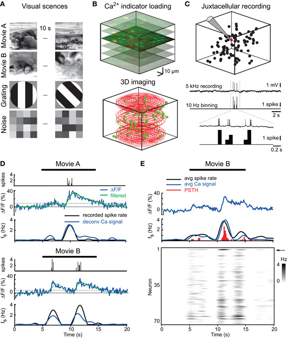
Figure 1. 3D calcium imaging of visual responses in layer 2/3 neuronal populations. (A) Stimulus set of visual scenes used in this study. (B) Top: Reference stack of a layer 2/3 cell population labeled with OGB 1 70–130 μm below pial surface (neurons green; astroglia counterstained with SR101, red). Bottom: 3D spiral scan trajectory used to collect data from layer 2/3 population. Neuron positions are indicated by green spheres. (C) Simultaneous 3D population imaging and single-cell juxtacellular recording. Top: 3D reconstruction of the imaged neurons with recorded neuron in red. Bottom: Juxtacellular recorded spikes binned to same sample rate as imaging data (10 Hz). (D) Example responses to Movie A and B with binned spikes (top) and simultaneously imaged fluorescence transients (middle; raw data in blue; filtered data in green). Dotted line indicates the 95th percentile of baseline. Bottom traces show estimated spike rates obtained by deconvolving calcium signal (blue) superimposed with the filtered actually recorded spike rates (black). (E) Average response to 10 consecutive Movie B presentations in a juxtacellularly recorded neuron and the surrounding population. Top: Mean traces for raw and deconvolved calcium signal, filtered spike rate, and peri-stimulus time histogram (PSTH) for the recorded neuron. Bottom: Intensity graph showing the average population response (recorded cell indicated by arrow).

3D Two-Photon Calcium Imaging

Calcium transients were acquired using a custom-built two-photon microscope equipped with a piezoelectric focusing unit (PIFOC; Physical Instruments, Germany) and a 40x water immersion objective (LUMPlanFl/IR; 0.8 NA; Olympus). 3D laser scanning and data acquisition were performed as described (Göbel et al., 2007) using custom written software (LabView; National Instruments, USA). A spiral scan line (10,000 scan points) was adjusted to cover a scan volume of 100–200 μm side length and 60–150 μm in depth usually starting at 100 μm below the cortical surface (Figure 1B). Fluorescence data were acquired together with the position signal of the scanning mirrors and the piezo focusing unit. On average 84 ± 5% (n = 12 populations) of the manually identified neurons were hit by the 3D scan line at 10 Hz scan rate.

Electrophysiology

For verification of the estimated spike rates we performed simultaneous juxtacellular recordings of neuronal firing patterns during 3D population imaging. A glass pipette was filled with NRR and the red dye Alexa 594 (20 μM; Invitrogen) for visualization. The tip of the pipette was placed near a neuron filled with calcium indicator and a seal was formed to record extracellular spikes. Spikes were recorded at 5 kHz using a patch-clamp amplifier (npi, Reutlingen, Germany) and Spike2 software (CED, Cambridge, UK), threshold detected and binned at the same rate as the imaging sample rate (10 Hz; Figure 1C).

Calcium Signal Analysis

Data were analyzed with LabView and Matlab (Mathworks, USA). Cells were detected manually in the reference stacks and their locations superimposed with the acquired position signal of the 3D laser scan line (Figure 1B). A volume of interest was placed around the cell bodies and the enclosed pixels of the scan line were assigned to the respective cell (Göbel et al., 2007). Relative percentage changes in fluorescence (ΔF/F) were thresholded at 95% confidence level of the baseline. To estimate the underlying spike rate we used a deconvolution method (Yaksi and Friedrich, 2006). Traces were low-pass filtered (0.4 Hz) and deconvolved with an idealized spike-evoked calcium transient (amplitude 5%, decay 1.6 seconds) (Figure 1D). Population responses are shown as intensity graphs, with time running on the horizontal axis and the estimated neuronal spike rate for all neurons depicted in the rows using a gray-scale code (Figure 1E).

To test the reliability of the neuronal responses to the presented visual stimuli we calculated the correlation of each trial to every other trial. This analysis was performed either for individual neurons or for the entire population, in which case all single-neuron responses (rows in the intensity graphs) were concatenated to a single long vector. The correlation of trial i and trial j of either single-neuron or network responses was calculated as the covariance of the two vectors (X_i, X_j), normalized by their respective variability (standard deviation, σ_i and σ_j):

Because visual scenes were presented in random order, we sorted the trials according to which visual scene had been presented and displayed the results in a correlation matrix with the correlation coefficient color-coded.

Decoding Analysis

We analyzed how well visual scenes could be decoded from the temporal response pattern either of individual neurons, the entire local population, or subsets of the population. Response trials were classified as encoding for one of the four visual scenes using a nearest mean classifier (Duin, 1996; Goard and Dan, 2009). We computed the class mean for each of the four visual scenes from the training set leaving out the tested trial. The assignment of a trial to a particular class was based on the nearest class mean using a correlation-based distance metric (d_ik = 1 − r_ik) where r_ik is the correlation of the test trial with the mean of stimulus class k. The obtained list of assigned stimulus identities was compared to the actual order of the stimulus presentation to get the percentage of correctly classified trials for each experiment and stimulus. The same procedure was used for single-cell correlations. Reliable responders were defined as neurons whose responses could be correctly classified in >50% of the trials for at least one visual scene. The type of stimulus preference of each reliable responder (single-stimulus versus multi-stimuli preference) was given by the number of those visual scenes with >50% correctly classified response trials.

To test the dependence of decoding performance on the size of the considered population we repeated the classification algorithm for variable-sized sub-networks of subsets of neurons randomly drawn from the total population of neurons in each experiment. This process was repeated 1000 times for each sub-network size (one to total number of neurons in experiment) to calculate the mean percentage of correctly classified trials for each network size. For each experiment the maximum performance was calculated as the percentage of correctly classified trials of the complete network. The minimum network size for reaching near-optimal decoding was defined as the mean number of cells required to reach 95% of maximum performance.

To test for dependence of decoding performance on number of discriminated stimuli, the same process was also applied to trials with responses to 2, 3, or 4 randomly drawn visual scenes (i.e., all six possible combinations were considered for 2 stimuli sets and four combinations for 3 stimuli). In addition, to correct for the dependence of information content on the number of stimuli tested, we repeated the analysis using mutual information as performance measure. Mutual information (in bits) of a decoded response vector R and stimulus vector S was calculated as

where p(r, s) denotes the joint probability distribution function and p(r) and p(s) the marginal probability distribution functions given the considered stimulus set M (e.g., [1,2,3,4] for discrimination of the 4 stimuli).

Neighborhood Analysis

We analyzed the spatial organization of functional responses within the local neuronal network. Cell positions in 3D coordinates were obtained from the reference stacks and were used to calculate distances between all cells. Inter-cell distances were binned with 20 μm bin size to reduce the occurrences of empty bins. A consistent analysis of local network organization required equal numbers of cells in each network. Therefore, we defined two neighborhood groups of neurons composed of the four nearest neighbors of a center neuron (“nearest neighbors”) or the next neighbors 5–8 (“second-nearest neighbors”). For these two groups of neighbors we evaluated the percentage of “functional clusters,” defined as neighbor groups with at least one member sharing the same stimulus preference as the center neuron. As a control, we calculated the percentage of functional clusters for randomly shuffled cell positions (repeated 1000 times). To calculate the decoding performance of local clusters we grouped each cell with its nearest and second-nearest neighborhoods and obtained the percentage of correctly classified trials using the trial classification method as described above.

Data are presented as mean ± standard error if not otherwise noted. Statistical significance was tested with a Student's t-test and significance level was 5% unless noted otherwise. Selectivity for individual stimuli was tested with one-way ANOVA.

Results

3D Population Imaging of Cortical Responses to Visual Scene Presentation

To examine the representation of visual scenes in mouse visual cortex we measured visually evoked 3D population activity in cortical layer 2/3 using two-photon calcium imaging. The stimulus set consisted of four 10 seconds movies representing different visual scenes (Figure 1A). All scenes were presented in random order to detect stimulus-specific cortical population responses irrespective of reported influences of previous stimulus history (Nikolic et al., 2009). Somatic calcium transients in neuronal populations were measured with the calcium indicator OGB-1 using 3D laser scanning (Göbel et al., 2007) (Figure 1B; see Methods; n = 12 populations from eight mice; 70–150 neurons per population). A deconvolution-based algorithm was used to convert calcium signals into an estimated time course of neuronal spike rate (Yaksi and Friedrich, 2006). We validated this approach with simultaneous juxtacellular recording of neuronal firing patterns during 3D population imaging (Figure 1C). Although single-spike sensitivity was not reached, the spike rates estimated by deconvolving the calcium transients fitted closely the simultaneously recorded spike patterns, filtered at the same frequency as the calcium data (Figure 1D). In addition, the average deconvolved response matched closely the average instantaneous spike rate and the peri-stimulus time histogram (PSTH) across trials (Figure 1E). Finally, the deconvolved calcium transients were highly correlated with the simultaneously recorded neuronal spike rate (0.74 ± 0.1; n = 7 neurons), significantly higher than the correlation of the raw fluorescence traces with the firing rate (0.43 ± 0.06; p < 0.0001). These findings indicate that the measured calcium transients represent the underlying neuronal firing patterns and that the deconvolved calcium transients are reliable estimates of neuronal spike rates. We therefore, used the estimated spike rates in the further analysis.

3D population imaging revealed highly reliable and specific stimulus-evoked activity patterns in neuronal subsets (Figure 2). For each stimulus about half of the neuronal population showed significant responses (Movie A: 55 ± 6%; Movie B: 48 ± 6%; Gratings: 55 ± 7%; Noise: 53 ± 5%; n = 1360 neurons in total). Typically, responsive neurons displayed several epochs of activation during presentation of one or multiple visual scenes, which were consistent across trials. To analyze the response specificity we calculated trial-to-trial correlations for all trial combinations with same or different stimuli, considering the neuronal responses of either the entire recorded population or individual neurons (Figures 3, 4; Methods). For entire populations, trial-to-trial correlations were computed from the respective intensity graphs and composed into a 2D matrix (Figures 3A,B). Correlations were significantly higher for same stimulus trials than for trials with different stimuli (example population in Figure 3C; pooled analysis in Figure 3D; mean correlation 0.18 ± 0.13 for n = 1891 same stimulus trial combinations, and 0.08 ± 0.09 for n = 5795 different stimulus trial combinations; ± SD; p < 0.001; t-test). Similar response specificity was observed for all visual scenes tested (mean correlation 0.21 ± 0.15, 0.14 ± 0.11, 0.21 ± 0.12, 0.16 ± 0.1 for Movie A, Movie B, Grating, and Noise, respectively). Hence, using 3D calcium imaging of layer 2/3 populations we could resolve specific neural network responses to the different presented visual scenes.

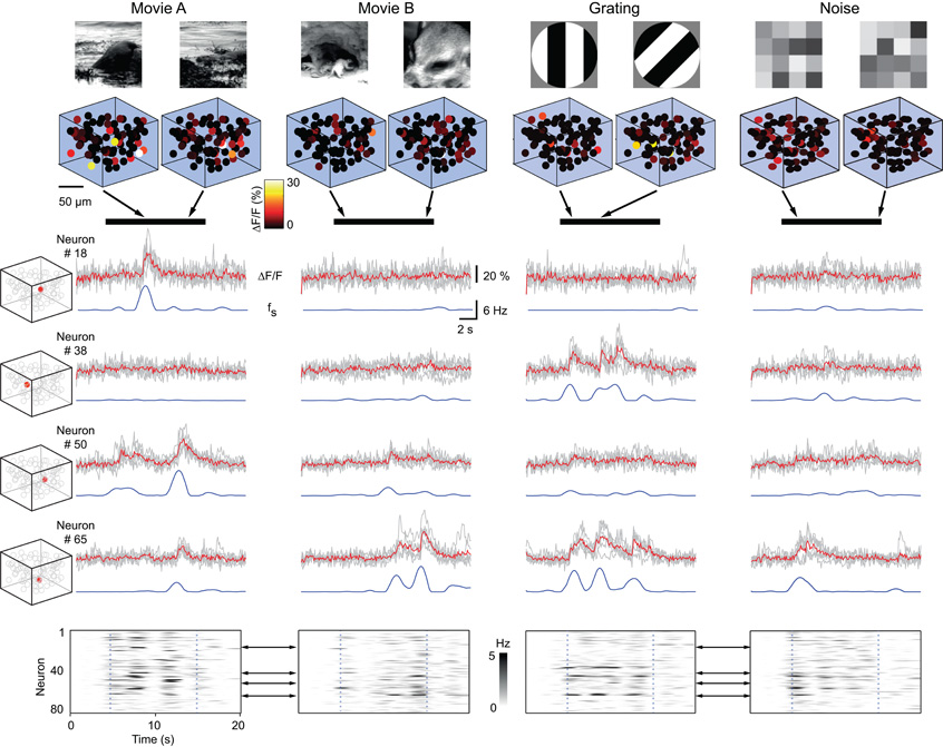
Figure 2. Reliable and specific activation of 3D populations by visual scenes. Upper rows: Example 3D activation pattern for two time points (arrows) during the presentation of Movie A, Movie B, Grating, and Noise stimulus (black bars). Middle rows: Example responses of four neurons (locations indicated by inserted box plots) to repeated stimulation with different visual scenes. Average relative fluorescence changes (ΔF/F) from six trials are shown together with the individual trials (grays). Blue traces are the estimated underlying spike rates (f_s). Bottom row: Intensity graphs showing the average firing rate of the entire population (rows represent individual neurons; time runs on the horizontal axis). Start and end of visual stimulation are indicated by dotted lines. Black arrows indicate example neurons.

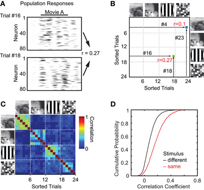
Figure 3. Response specificity of local population. (A) and (B) Method to calculate trial-to-trial correlation matrix. (A) Population trial-to-trial correlations were obtained by correlating all pairs of trials of entire population responses to visual scenes. (B) The correlation matrix was filled with pair-wise correlation coefficients of f_s responses for each pair of trials. The example shows six trials per presented visual scene. Trials are sorted by the presented visual scenes indicated on right and top. (C) Trial correlation matrix for entire network response of the population shown in Figure 2. Dashed white lines separate trials with different visual scenes indicated on the left and top. (D) Cumulative distribution of correlation coefficients from the population analysis for all experiments with trials with same visual stimulus (red) or with different visual stimuli (black). Trial-to-trial correlations were significantly higher for same stimulus trials compared to different stimulus trials.

Correlation analysis of single-cell response trials revealed features distinct from the population responses (Figures 4A,B). While some neurons responded primarily during only one of the visual scenes (e.g., neuron #18 and #38) other neurons showed distinct responses to two or more stimuli (e.g., neuron #65). The diversity of responses from individual cells resulted in broader and overlapping distributions of trial-to-trial correlations for same stimulus trials and different stimulus trials (Figure 4C; mean correlation 0.14 ± 0.39 for n = 82,120 same-stimulus trial combinations and 0.04 ± 0.36 for n = 2,54,220 different stimulus trial combinations in 403 cells; ± SD; p < 0.001, t-test). We conclude that individual layer 2/3 neurons may be recruited only by specific visual scenes, raising the question how well visual scenes can be decoded from temporal response patterns in single-neurons versus multiple neurons within the local population.

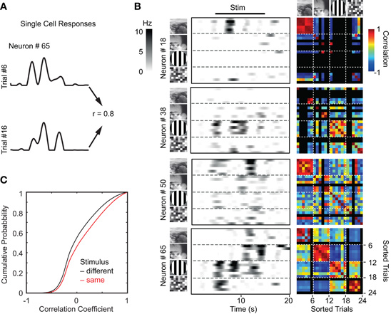
Figure 4. Response specificity of individual neurons. (A) Single-cell trial-to-trial correlations were obtained by correlating trials of individual cell responses to visual scenes. The example shows two trials from the same cell in response to a visual stimulus (Grating). Method to calculate trial correlation matrix is shown in Figure 3. (B) Spike rate intensity graphs and single-neuron trial correlation matrices for the example neurons shown in Figure 2. Black pixels indicate trials without responses to presented visual scenes. Trial order in spike rate intensity graphs and correlation matrices are the same. Dashed white lines separate trials with different visual scenes indicated on the left and top. (C) Cumulative distribution of correlation coefficients from single-cell analysis from all cells in all experiments for trials with same visual stimulus (red) or with different visual stimuli (black). Trial-to-trial correlation coefficients are from single-cell responses. To compare with network responses see Figure 3.

Decoding of Visual Scenes

For decoding visual scenes from the recorded responses we used a nearest mean classifier to predict from individual trials, which visual stimulus had been presented (see Methods). We considered either the entire sampled network (concatenating all single-neuron response vectors) or individual neurons. For each experiment, the response vectors for all trials were assigned to the clusters representing the different visual scenes (Figure 5A). The obtained list of assigned cluster identities was compared to the actual order of the scene presentation, yielding the percentage of correctly classified trials for each experiment and stimulus. Pooled across all experiments, 84 ± 4% of the trials on average were correctly classified with similar success rates for the different visual scenes (Figure 5C; 92 ± 4%, 82 ± 7%, 86 ± 6%, and 75 ± 6% for Movie A, Movie B, Grating, and Noise, respectively; p = 0.26, ANOVA). On the individual cell level we defined “reliable responders” as cells that correctly predicted the stimulus in >50% of the trials for at least one visual scene (Figure 5B). About half of the responding cells were such reliable responders (26 ± 5% of total number of cells) with most of them preferring only one particular visual scene (75 ± 4% of reliable responders; n = 12 populations) and only a minority showing reliable responses to multiple scenes (Figure 5D; according to this definition example neurons #18 and #38 in Figure 4 had single-scene preference for Movie A and the Grating movie, respectively; neuron #50 reliably responded to Movies A and B; and neuron #65 responded to all four visual scenes).

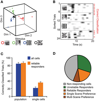
Figure 5. Decoding of visual scenes from 3D population and single-cell responses. (A) Trial classification by nearest mean clustering of population or single-cell responses. Example shows dimension-reduced population response for better visibility (Dim 1–3). Each visual scene was presented six times and corresponding trials were correctly classified. The crosses indicate the average responses (see Methods). (B) Example of single-cell responses to different visual scenes. Correctly classified trials are indicated by red tick marks. Cells with >50% correctly classified trials for any presented visual scene were classified as “reliable responders” to this particular scene. Example cell was classified as reliable responder to all four presented visual scenes. (C) Percentage of correctly classified trials for all population and single-cell responses comprising either all cells or reliably responding neurons only. (D) Pie-chart grouping neurons according to their response properties, pooled over all experiments. Reliable responders are further subdivided into single-scene and multi-scene preferring neurons. Note that the majority of reliable responders show single-scene preference.

Applying the network decoding scheme to the sub-networks of reliable responders resulted in similar decoding performance as the entire population (86 ± 3%; Figure 5C). In contrast, when we applied the decoding scheme to individual neurons, performance was dramatically decreased (Figure 5C). The average single-cell performance pooled for all cells was close to the 25% chance level (21 ± 3%) and pooling over only the reliable responders also resulted in a reduced decoding performance (35 ± 2% correctly classified trials). The likely explanation is that most reliable responder's preferred only one specific visual scene and thus were “blind” to the other scenes. These results show that individual neurons can be highly tuned to specific features of the visual input. However, only by observing the cooperation of several neurons within the population, increasing the likelihood to sample from distinct functional sub-networks, it is possible to decode the cortical representation of the visual scenes.

Dependence on Network Size and Number of Stimuli

To inquire how the decoding performance of the local neuronal population depends on the number of discriminated visual scenes we repeated the decoding analysis, selecting trials to include only 2, 3, or 4 different visual scenes. Moreover, in order to establish the minimum number of cells that have to be considered to reach near-optimal (95%) decoding performance, we examined how the fraction of correctly classified trials depends on the number of cells included in the analysis. Figure 6A illustrates this analysis for one example population that reached 100% performance for >100 neurons. Averaged over all populations, the maximal decoding performance was independent of whether 2, 3, or 4 different visual scenes were considered (Figure 6B; 92 ± 2%, 88 ± 3%, and 85 ± 5%, respectively; n = 12; p = 0.2; ANOVA). Similar decoding performance levels were also reached for the sub-networks of reliable responders (Figure 6B; 93 ± 2%, 89 ± 3%, and 87 ± 3% for 2, 3, or 4 different visual scenes, respectively; p = 0.3) and only 10–20 reliable responders were required to reach 95% decoding level (Figure 6C). On the other hand, drawing cells randomly from the entire population required larger number of cells: at least 52, 64, and 69 simultaneously recorded neurons were required to reach 95% decoding performance for 2, 3, and 4 different visual scenes, respectively (Figure 6C).

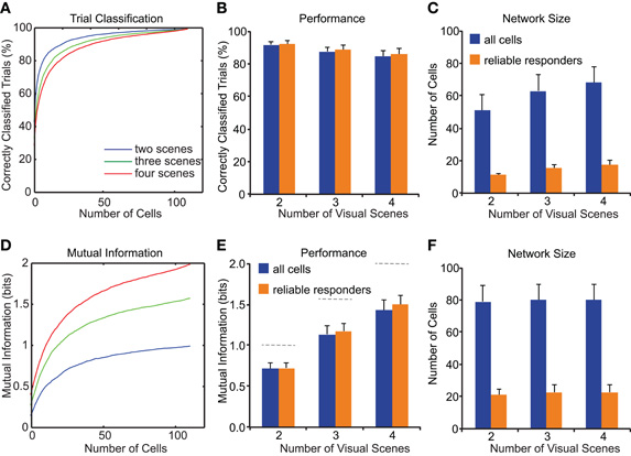
Figure 6. Dependence of decoding performance on network size and number of stimuli. (A–C) Decoding performance is measured as percentage of correctly classified trials as shown in Figure 5 and Methods. (A) The percentage of correctly classified trials increases with growing population size in an example experiment. Different colored lines show discrimination of 2, 3, or 4 different visual scenes. (B) Average decoding performance across all experiments depends on number of discriminated visual scenes but is similar for entire population (blue) and networks of reliable responders alone (orange). (C) Required network size for near-optimal decoding depends on the number of discriminated visual scenes. Note that assembling networks of reliable responders alone reduces the required network size. (D–E) Decoding performance measured as mutual information. (D) Mutual information increases with growing population size in same example experiment as in (A). (E) Average decoding performance as in (B) corrected for mutual information content. Note that maximum mutual information depends on the number of visual scenes to discriminate (1, 1.58, and 2 bits, respectively; dashed lines). (F) Required network size to obtain near-optimal information is independent of number of discriminated visual scenes.

The finding that the smallest required network size depended on the number of different visual scenes to classify might simply be due to the different information content when discriminating different numbers of visual scenes. For example, chance level is 50% for 2 visual scenes whereas it is 25% for 4 different scenes. To take this difference in information content into account we also used mutual information as performance measure, a quantity that measures the reduction in uncertainty about the presented visual scene by knowledge of a single-trial neuronal response. Mutual information increased with growing population size and reached higher levels when a larger number of scenes had to be discriminated (Figures 6D,E; 0.7 ± 0.1 bits, 1.1 ± 0.1 bits, and 1.4 ± 0.1 bits for 2, 3, or 4 different visual scenes, respectively). Similar results were obtained for populations consisting either of the entire imaged population or only of the reliable responders (Figure 6E). Calculating the network size required to reach near-optimal (95%) mutual information in each experiment resulted in similar numbers of cells for different numbers of visual scenes (Figure 6F; 79 ± 10, 81 ± 10, and 80 ± 10 for 2, 3, and 4 visual scenes, respectively; p = 1.0, ANOVA). Selecting only the reliable responders reduced the minimal population size consistently to 21 ± 3, 23 ± 4, 23 ± 4 for 2, 3, and 4 visual scenes, respectively (Figure 6F; p = 0.9). These findings indicate that observing the neuronal representations in about 80 randomly picked layer 2/3 neurons is required to discriminate low numbers of visual scenes with high fidelity, while around 20 neurons suffice if only the sub-network of reliable responders is considered. However, previous knowledge about the identity and location of these neurons is required to selectively collect information from this subset. Therefore, we further elaborated these findings by analyzing the spatial relationship of the reliably responding neurons.

Spatial Organization of Visual Scene Representations

The 3D laser scanning technique not only acquires population responses to dynamic visual stimuli, it further provides 3D spatial information about the location of the sampled neurons. Hence, we analyzed the relationship between spatial location and stimulus preference for all neurons in the imaged populations (Figure 7A). We evaluated the abundance of pairs of neurons in the data sets having same or different stimulus preferences and compared these values to those from the same data sets with shuffled neuron positions. Relative to random, we found a significantly higher probability of neuron pairs with the same stimulus preference being in close proximity (48 ± 25% and 18 ± 8% for distances of 20 and 40 μm, respectively; n = 12; p = 0.01; t-test). For pairs of neurons with different stimulus preferences the abundance was similar to the calculated random probability (Figure 7B).

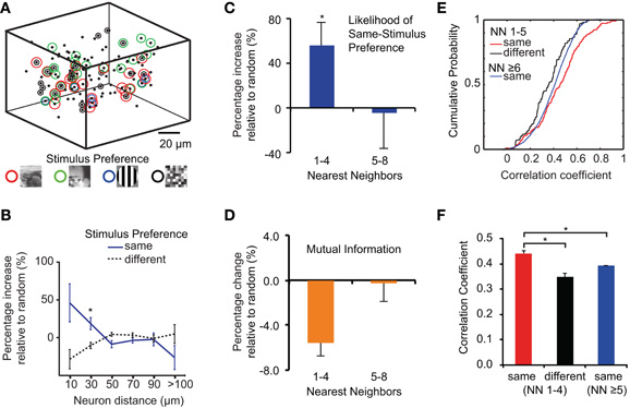
Figure 7. Spatial organization of 3D population responses to different visual scenes. (A) Example of 3D distribution of neuronal stimulus preference. Note that few neurons reliably respond to more than one visual scene. (B) Occurrences of neurons with same or different stimulus preferences at different cell-to-cell distances compared to shuffled data sets. Neurons have significantly more neighbors with the same visual scene preference at distances of up to 40 μm than neighbors with different scene preferences. (C) Occurrences of functional clusters of nearest neighbors with same stimulus preference compared to shuffled data sets. (D) Decoding performance for different clusters of nearest neighbors compared to randomly picked groups of five cells. (E) Cumulative distributions of correlation coefficients between cells with different stimulus preferences and spatial locations. “NN 1-4” indicates correlations with the first four nearest neighbors, “NN ≥5” indicates correlations with neurons further away. (F) Average correlation coefficients between neurons are highest for neurons with preference for the same visual scene and located within local clusters.

Because the number of neurons differed within local volumes defined by a fixed radius, we performed a neighborhood analysis, considering a nearest neighbors group (four closest cells) and a second-nearest neighborhood (neighbors 5–8). The average distance of each cell to its fourth nearest neighbor was 21 ± 6 μm (95th percentile: 32 μm). We examined the fine-scale spatial organization of the population responses by counting for each reliable responder the number of neurons in the neighborhood that displayed the same visual scene preference as this particular neuron and compared the results to the same data set with shuffled cell positions (Figures 7B,C). The nearest neighbors group displayed a 50% higher probability of comprising at least one neuron with the same stimulus preference as the center neuron compared to randomly shuffled networks (Figure 7C; 47 ± 7%; n = 12 experiments; p = 0.01; t-test). No significant increase was found when considering the second-nearest neighbors group (p = 0.8). This finding indicates that there exists a certain redundancy of stimulus coding in clusters of neighboring neurons, which might deteriorate decoding performance. Indeed, calculating the mutual information of each neuron's response together with its four nearest neighbors showed a significant decrease by about 6% compared to randomly picking groups of six cells (Figure 7D; 0.53 ± 0.05 bits and 0.56 ± 0.056 bits for neighboring neurons and for random groups of cells, respectively; p = 0.001; n = 12 experiments; t-test). Again, no significant difference in decoding performance was found for the second-nearest neighbors group (p = 0.98).

Local neighbors with the same stimulus preference could still exhibit quite different temporal response profiles or, alternatively, also show increased temporal correlations. To examine this question, we compared the inter-neuron correlation coefficients for neuron pairs within the nearest neighbors group, showing either same or different stimulus preference. In addition, we analyzed neuron pairs with the same stimulus preference but located either within nearest neighbors group or further away from each other. The local neighbors with same stimulus preference displayed the highest correlation coefficients, with the mean being significantly higher compared to the two other controls (Figures 7E,F; mean correlation 0.44 ± 0.21, 0.35 ± 0.17, 0.4 ± 0.16 for local neighbors with same and different stimulus preference and far neighbors, respectively; ± SD; p < 0.001 for both comparisons with different stimulus and far neighbors controls; t-test). These results indicate that neurons within local clusters are more correlated to each other than to neurons further away even if those share the same stimulus preference. Nearby neurons in layer 2/3 of mouse visual cortex thus tends to share dynamic tuning properties.

Discussion

Using 3D two-photon calcium imaging we characterized neuronal spiking activity of layer 2/3 populations in mouse visual cortex during presentations of a set of dynamic visual scenes. We found stimulus-specific response patterns in neuronal subsets with most responding neurons preferring mainly one visual scene. The presented visual scene could be well decoded from the population activity pattern, requiring only about 20 neurons when the most informative pool of reliable responders was considered. Spatial analysis furthermore suggests that within local neighborhoods there exist functional sub-networks of neurons that share similar response properties. Our findings provide novel insights into how the visual environment is dynamically represented in the local microcircuit of mouse neocortex.

3D Two-Photon Calcium Imaging in Visual Cortex

Several recent studies employed two-photon calcium imaging to investigate the functional microcircuit of visual cortex. Often, drifting gratings were applied as visual stimuli to map orientation tuning using standard frame imaging (Ohki et al., 2005, 2006; Mrsic-Flogel et al., 2007; Sohya et al., 2007; Li et al., 2008; Kara and Boyd, 2009; Ch'ng and Reid, 2010; Kerlin et al., 2010; Runyan et al., 2010) or imaging of small volumes (Andermann et al., 2010; Kerlin et al., 2010). Here, we applied 3D laser spiral scanning (Göbel et al., 2007) to reveal dynamic response patterns simultaneously in rather large volumes. Despite the reduced temporal resolution and signal-to-noise ratio compared to electrophysiological techniques, we confirmed using simultaneous juxtacellular recordings that 3D calcium imaging faithfully resolves visually evoked neuronal firing patterns (Figure 1). 3D imaging is particularly beneficial for studying the dynamic 3D representation of specific stimuli as well as analyzing spatial functional relationships within local populations. Here, it enabled us to reveal complete representations in local neighborhoods whereas microelectrodes sample only from very few neurons within a volume of 100 μm diameter (Henze et al., 2000). In addition, 3D imaging permitted us to identify the functionally relevant subset of reliable responders, which are generally dispersed throughout the volume, and examine their decoding performance.

While most of our current concepts of visual processing have come from experiments using artificial stimulus sets, it is important to use natural stimuli to work out how the brain processes the input it is usually confronted with (Felsen and Dan, 2005; Olshausen and Field 2005). Interestingly, in cats, with their highly columnar organization of visual cortex (Ohki et al., 2006), responses to natural scenes were heterogeneous in presumed nearby neurons (Yen et al., 2007). In addition, feature detection in visual scenes is increased when these features are presented as parts of natural scenes rather than as artificial stimuli (Felsen et al., 2005). Moreover, it has been demonstrated that temporal patterns of population activity serve well to differentiate between natural stimuli, noise, and gratings (Kayser et al., 2003). These results point to a distinct visual-coding strategy that is tuned to the dynamics of natural scenes.

Functional Micro-Organization of Mouse Visual Cortex

We found a subset of the neurons in each population to respond reliably to visual scene stimulation (Figures 4, 5). The majority of these neurons preferred only one particular scene providing further evidence that neurons in mouse visual cortex can be highly selective to visual features (Niell and Stryker, 2008). In addition, neighboring neurons tended to share the same stimulus preference suggesting the existence of functional sub-networks. In another recent two-photon imaging study in mouse visual cortex, receptive field sub-regions were found to highly overlap even for neurons separated by several hundred microns (Smith and Hausser, 2010). Considering an average receptive field diameter of 10–14° for pyramidal neurons in mouse visual cortex (Niell and Stryker, 2008; Gao et al., 2010; Smith and Hausser, 2010) and a cortical magnification factor of 15 μm/° (Schuett et al., 2002), receptive fields of neurons within a cortical volume of 100 μm are also expected to be highly overlapping. It is therefore, unlikely that visual scene preference observed in our study is simply explained by different spatial locations of the receptive fields. More likely, stimulation of visual field areas surrounding the neurons' receptive fields caused modulatory influences (Vinje and Gallant, 2000; Angelucci and Bullier, 2003). This can lead to the observed decorrelation of the population responses and also to an increase in the information capacity (Vinje and Gallant, 2000, 2002).

Despite the seemingly random (“salt-and-pepper”) organization of orientation tuning in rodent visual cortex (Ohki and Reid, 2007) our spatial analysis of the local representation of visual scenes indicates a certain degree of functional clustering on the scale of ∼40 μm or of the nearest five neighboring cells (Figure 7). It has been reported that cortical neurons form mini-columns with similar widths of 20–40 μm across species (Raghanti et al., 2010). Local neighbors within 50 μm also share a higher connectivity (Holmgren et al., 2003) making it likely that the observed clusters represent interconnected sub-networks, with neurons sharing common sensory inputs from layer 4 afferents (Yoshimura et al., 2005). To determine the connectivity scheme of the entire population a serial sectioning electron-microscopy study would be required. While this technique has been applied to reconstruct the connectivity of few identified neurons in mouse visual cortex (Bock et al., 2011), it is still far from reconstructing the full circuitry of a hundred neurons as in our 3D populations. However, a recent study has shown that neighboring neurons with high response correlations to natural scenes are also more likely to be connected to each other (Ko et al., 2011). Indeed, we find members of local clusters with similar stimulus preferences to be more correlated to each other in their responses to visual scenes than neurons with different stimulus preferences or neurons further apart from each other (Figures 7E,F).

These findings are consistent with the idea that the local clusters observed in our study could represent interconnected sub-networks sharing similar sensory inputs and therefore, similar tuning properties. The redundancy of encoded information in such local sub-networks reduces their discriminative power to distinguish different visual scenes. Consequently, decoding of the visual scenery improves by integration over several, spatially segregated sub-networks. Such a microcircuit, where follower networks integrate inputs from several distinct sub-networks, has recently been reported and proposed for sensory feature integration (Kampa et al., 2006). Thus, 3D imaging of network responses to dynamic visual scenes suggests a population code in layer 2/3 of visual cortex, where the visual environment is represented in the spatio-temporal activation patterns of distinct neuronal sub-networks.

Decoding of Visual Scenes

Our results show that cortical neurons can express diverse tuning properties in response to dynamic visual scenes. This is, to our knowledge, the first study investigating the decoding properties of complete and unbiased local populations using dynamic naturalistic visual stimuli. Even though visual scene-evoked activity was distributed and sparse, we found that population responses were specific and reliable so that in more than 80% of the trials activity patterns could be correctly assigned to one of the four presented visual scenes (Figure 5). Such high level of decoding could be achieved with population sizes of about 50–70 neurons from the total pool and 10–20 neurons from the pool of reliably responding neurons depending on whether 2, 3, or 4 different visual scenes were discriminated (Figure 6). Interestingly, correcting for the difference in information obtained from discrimination of different numbers stimuli led to a similar required population size of ∼80 neurons or ∼20 reliable responders for all numbers of visual scenes (Figure 6). This implies that the information provided by each neuron is independent of the number of discriminated stimuli, which can be explained by the fact that most neurons encode only one particular visual scene. It should, however, be noted that this study is not exhaustive in the sample set of different visual scenes or in their duration. Presentations of longer movies would also increase the diversity of presented stimulus features and therefore, the probability of neurons to respond. Nonetheless, similar decoding levels have been reached in primate visual cortex during a face discrimination task using comparable numbers of selected reliably responding neurons (Rolls et al., 1997). Interestingly, our observed minimal population size is also similar to reports of required network sizes for motor movement prediction (Lebedev et al., 2008). These results and the high success rate of single-trial classification further confirm the fidelity of our 3D imaging technique. Consequently, with 3D imaging, we have the capacity to resolve the representation of visual scenes in local microcircuits.

Future Directions

A number of opportunities exist to reveal further details of the functional organization of cortical microcircuits. For example, using a novel high-speed imaging technique, we demonstrated precise reconstruction of the sparse activation of visual cortex neurons during natural movie presentation (Grewe et al., 2010). A further extension of this method to 3D (Cheng et al., 2011; Grewe et al., 2011) should make it possible to reveal 3D activation patterns at higher temporal resolution. Second, discrimination of neuronal subclasses is desirable (Ascoli et al., 2008), and is becoming possible through post-hoc immunostaining methods (Kerlin et al., 2010). Third, genetically encoded calcium indicators have become nearly as sensitive as synthetic indicators (Lutcke et al., 2010), and enable chronic recordings from the same neuronal populations over weeks to months (Mank et al., 2008; Tian et al., 2009), to explore the effect of behavior and attention on the cortical representation of visual scenes (Andermann et al., 2010). Together, two-photon imaging of local representations of dynamic natural scenes in mouse visual cortex is a powerful approach to study the function of visual cortex in a realistic context.

Conflict of Interest Statement

The authors declare that the research was conducted in the absence of any commercial or financial relationships that could be construed as a potential conflict of interest.

Acknowledgments

This work was supported by the Swiss National Science Foundation (Grant Nr. 31-120480 to Björn M. Kampa) and the University of Zurich (Forschungskredit to Björn M. Kampa and Morgane M. Roth), the EU-FP7 program (project 243914, Brain-i-Nets, to Fritjof Helmchen) and the Swiss SystemsX.ch initiative (project 2008/2011-Neurochoice, to Fritjof Helmchen). We would like to thank Johannes Letzkus, Florent Haiss, Henry Lütcke, Dylan Muir, and Nuno da Costa for their comments on earlier versions of this manuscript.

References

Andermann, M. L., Kerlin, A. M., and Reid, R. C. (2010). Chronic cellular imaging of mouse visual cortex during operant behavior and passive viewing. Front. Cell. Neurosci. 4, 3. doi: 10.3389/fncel.2010.00003
Angelucci, A., and Bullier, J. (2003). Reaching beyond the classical receptive field of V1 neurons: horizontal or feedback axons? J. Physiol. Paris 97, 141–154.
Ascoli, G. A., Alonso-Nanclares, L., Anderson, S. A., Barrionuevo, G., Benavides-Piccione, R., Burkhalter, A., Buzsáki, G., Cauli, B., Defelipe, J., Fairén, A., Feldmeyer, D., Fishell, G., Fregnac, Y., Freund, T. F., Gardner, D., Gardner, E. P., Goldberg, J. H., Helmstaedter, M., Hestrin, S., Karube, F., Kisvárday, Z. F., Lambolez, B., Lewis, D. A., Marin, O., Markram, H., Muñoz, A., Packer, A., Petersen, C. C., Rockland, K. S., Rossier, J., Rudy, B., Somogyi, P., Staiger, J. F., Tamas, G., Thomson, A. M., Toledo-Rodriguez, M., Wang, Y., West, D. C., Yuste, R. (2008). Petilla terminology: nomenclature of features of GABAergic interneurons of the cerebral cortex. Nat. Rev. Neurosci. 9, 557–568.
Bock, D. D., Lee, W. C., Kerlin, A. M., Andermann, M. L., Hood, G., Wetzel, A. W., Yurgenson, S., Soucy, E. R., Kim, H. S., and Reid, R. C. (2011). Network anatomy and in vivo physiology of visual cortical neurons. Nature 471, 177–182.
Ch'ng, Y. H., and Reid, R. C. (2010). Cellular imaging of visual cortex reveals the spatial and functional organization of spontaneous activity. Front. Integr. Neurosci. 4, 20. doi: 10.3389/fnint.2010.00020
Cheng, A., Goncalves, J. T., Golshani, P., Arisaka, K., and Portera-Cailliau, C. (2011). Simultaneous two-photon calcium imaging at different depths with spatiotemporal multiplexing. Nat. Methods 8, 139–142.
Felsen, G., Touryan, J., Han, F., and Dan, Y. (2005). Cortical sensitivity to visual features in natural scenes. PLoS Biol. 3, e342. doi: 10.1371/journal.pbio.0030342
Gao, E., DeAngelis, G. C., and Burkhalter, A. (2010). Parallel input channels to mouse primary visual cortex. J. Neurosci. 30, 5912–5926.
Goard, M., and Dan, Y. (2009). Basal forebrain activation enhances cortical coding of natural scenes. Nat. Neurosci. 12, 1444–1449.
Göbel, W., Kampa, B. M., and Helmchen, F. (2007). Imaging cellular network dynamics in three dimensions using fast 3D laser scanning. Nat. Methods 4, 73–79.
Grewe, B. F., and Helmchen, F. (2009). Optical probing of neuronal ensemble activity. Curr. Opin. Neurobiol. 19, 520–529.
Grewe, B. F., Langer, D., Kasper, H., Kampa, B. M., and Helmchen, F. (2010). High-speed in vivo calcium imaging reveals neuronal network activity with near-millisecond precision. Nat. Methods 7, 399–405.
Grewe, B. F., Voigt, F. F., van't Hoff, M., and Helmchen, F. (2011). Fast two-layer two-photon imaging of neuronal cell populations using an electrically tunable lens. Biomed. Opt. Express 2, 2035–2046.
Haider, B., Krause, M. R., Duque, A., Yu, Y., Touryan, J., Mazer, J. A., and McCormick, D. A. (2010). Synaptic and network mechanisms of sparse and reliable visual cortical activity during nonclassical receptive field stimulation. Neuron 65, 107–121.
Hellwig, B. (2000). A quantitative analysis of the local connectivity between pyramidal neurons in layers 2/3 of the rat visual cortex. Biol. Cybern. 82, 111–121.
Henze, D. A., Borhegyi, Z., Csicsvari, J., Mamiya, A., Harris, K. D., and Buzsaki, G. (2000). Intracellular features predicted by extracellular recordings in the hippocampus in vivo. J. Neurophysiol. 84, 390–400.
Holmgren, C., Harkany, T., Svennenfors, B., and Zilberter, Y. (2003). Pyramidal cell communication within local networks in layer 2/3 of rat neocortex. J. Physiol. 551, 139–153.
Jia, H., Rochefort, N. L., Chen, X., and Konnerth, A. (2010). Dendritic organization of sensory input to cortical neurons in vivo. Nature 464, 1307–1312.
Kampa, B. M., Letzkus, J. J., and Stuart, G. J. (2006). Cortical feed-forward networks for binding different streams of sensory information. Nat. Neurosci. 9, 1472–1473.
Kara, P., and Boyd, J. D. (2009). A micro-architecture for binocular disparity and ocular dominance in visual cortex. Nature 458, 627–631.
Kayser, C., Salazar, R. F., and König, P. (2003). Responses to natural scenes in cat V1. J. Neurophysiol. 90, 1910–1920.
Kerlin, A. M., Andermann, M. L., Berezovskii, V. K., and Reid, R. C. (2010). Broadly tuned response properties of diverse inhibitory neuron subtypes in mouse visual cortex. Neuron 67, 858–871.
Ko, H., Hofer, S. B., Pichler, B., Buchanan, K. A., Sjostrom, P. J., and Mrsic-Flogel, T. D. (2011). Functional specificity of local synaptic connections in neocortical networks. Nature 473, 87–91.
Lebedev, M. A., O'Doherty, J. E., and Nicolelis, M. A. (2008). Decoding of temporal intervals from cortical ensemble activity. J. Neurophysiol. 99, 166–186.
Li, Y., Van Hooser, S. D., Mazurek, M., White, L. E., and Fitzpatrick, D. (2008). Experience with moving visual stimuli drives the early development of cortical direction selectivity. Nature 456, 952–956.
Lutcke, H., Murayama, M., Hahn, T., Margolis, D. J., Astori, S., Zum Alten Borgloh, S. M., Gobel, W., Yang, Y., Tang, W., Kugler, S., Sprengel, R., Nagai, T., Miyawaki, A., Larkum, M. E., Helmchen, F., and Hasan, M. T. (2010). Optical recording of neuronal activity with a genetically-encoded calcium indicator in anesthetized and freely moving mice. Front. Neural Circuits 4, 9. doi: 10.3389/fncir.2010.00009
Mank, M., Santos, A. F., Direnberger, S., Mrsic-Flogel, T. D., Hofer, S. B., Stein, V., Hendel, T., Reiff, D. F., Levelt, C., Borst, A., Bonhoeffer, T., Hubener, M., and Griesbeck, O. (2008). A genetically encoded calcium indicator for chronic in vivo two-photon imaging. Nat. Methods 5, 805–811.
Markram, H., Wang, Y., and Tsodyks, M. (1998). Differential signaling via the same axon of neocortical pyramidal neurons. Proc. Natl. Acad. Sci. U.S.A. 95, 5323–5328.
Medini, P. (2011). Cell-type–specific sub- and suprathreshold receptive fields of layer 4 and layer 2/3 pyramids in rat primary visual cortex. Neuroscience 190, 112–126.
Mrsic-Flogel, T. D., Hofer, S. B., Ohki, K., Reid, R. C., Bonhoeffer, T., and Hubener, M. (2007). Homeostatic regulation of eye-specific responses in visual cortex during ocular dominance plasticity. Neuron 54, 961–972.
Niell, C. M., and Stryker, M. P. (2008). Highly selective receptive fields in mouse visual cortex. J. Neurosci. 28, 7520–7536.
Nikolic, D., Hausler, S., Singer, W., and Maass, W. (2009). Distributed fading memory for stimulus properties in the primary visual cortex. PLoS Biol. 7, e1000260. doi: 10.1371/journal.pbio.1000260
Nimmerjahn, A., Kirchhoff, F., Kerr, J. N., and Helmchen, F. (2004). Sulforhodamine 101 as a specific marker of astroglia in the neocortex in vivo. Nat. Methods 1, 31–37.
Ohki, K., and Reid, R. C. (2007). Specificity and randomness in the visual cortex. Curr. Opin. Neurobiol. 17, 401–407.
Ohki, K., Chung, S., Ch'ng, Y. H., Kara, P., and Reid, R. C. (2005). Functional imaging with cellular resolution reveals precise micro-architecture in visual cortex. Nature 433, 597–603.
Ohki, K., Chung, S., Kara, P., Hubener, M., Bonhoeffer, T., and Reid, R. C. (2006). Highly ordered arrangement of single neurons in orientation pinwheels. Nature 442, 925–928.
Olshausen, B. A., and Field, D. J. (2005). How close are we to understanding v1? Neural Comput. 17, 1665–1699.
Raghanti, M. A., Spocter, M. A., Butti, C., Hof, P. R., and Sherwood, C. C. (2010). A comparative perspective on minicolumns and inhibitory GABAergic interneurons in the neocortex. Front. Neuroanat. 4, 3. doi: 10.3389/neuro.05.003.2010
Rolls, E. T., Treves, A., and Tovee, M. J. (1997). The representational capacity of the distributed encoding of information provided by populations of neurons in primate temporal visual cortex. Exp. Brain Res. 114, 149–162.
Runyan, C. A., Schummers, J., Van Wart, A., Kuhlman, S. J., Wilson, N. R., Huang, Z. J., and Sur, M. (2010). Response features of parvalbumin-expressing interneurons suggest precise roles for subtypes of inhibition in visual cortex. Neuron 67, 847–857.
Schuett, S., Bonhoeffer, T., and Hubener, M. (2002). Mapping retinotopic structure in mouse visual cortex with optical imaging. J. Neurosci. 22, 6549–6559.
Smith, S. L., and Hausser, M. (2010). Parallel processing of visual space by neighboring neurons in mouse visual cortex. Nat. Neurosci. 13, 1144–1149.
Sohya, K., Kameyama, K., Yanagawa, Y., Obata, K., and Tsumoto, T. (2007). GABAergic neurons are less selective to stimulus orientation than excitatory neurons in layer II/III of visual cortex, as revealed by in vivo functional Ca2+ imaging in transgenic mice. J. Neurosci. 27, 2145–2149.
Stosiek, C., Garaschuk, O., Holthoff, K., and Konnerth, A. (2003). In vivo two-photon calcium imaging of neuronal networks. Proc. Natl. Acad. Sci. U.S.A. 100, 7319–7324.
Tian, L., Hires, S. A., Mao, T., Huber, D., Chiappe, M. E., Chalasani, S. H., Petreanu, L., Akerboom, J., McKinney, S. A., Schreiter, E. R., Bargmann, C. I., Jayaraman, V., Svoboda, K., and Looger, L. L. (2009). Imaging neural activity in worms, flies and mice with improved GCaMP calcium indicators. Nat. Methods 6, 875–881.
Tolhurst, D. J., Smyth, D., and Thompson, I. D. (2009). The sparseness of neuronal responses in ferret primary visual cortex. J. Neurosci. 29 2355–2370.
van Hateren, J. H., and Ruderman, D. L. (1998). Independent component analysis of natural image sequences yields spatio-temporal filters similar to simple cells in primary visual cortex. Proc. Biol. Sci. 265, 2315–2320.
Vinje, W. E., and Gallant, J. L. (2000). Sparse coding and decorrelation in primary visual cortex during natural vision. Science 287, 1273–1276.
Vinje, W. E., and Gallant, J. L. (2002). Natural stimulation of the nonclassical receptive field increases information transmission efficiency in V1. J. Neurosci. 22, 2904–2915.
Wallace, D. J., and Kerr, J. N. (2010). Chasing the cell assembly. Curr. Opin. Neurobiol. 20, 296–305.
Yaksi, E., and Friedrich, R. W. (2006). Reconstruction of firing rate changes across neuronal populations by temporally deconvolved Ca2+ imaging. Nat. Methods 3, 377–383.
Yao, H., Shi, L., Han, F., Gao, H., and Dan, Y. (2007). Rapid learning in cortical coding of visual scenes. Nat. Neurosci. 10, 772–778.
Yen, S. C., Baker, J., and Gray, C. M. (2007). Heterogeneity in the responses of adjacent neurons to natural stimuli in cat striate cortex. J. Neurophysiol. 97, 1326–1341.
Keywords: neocortex, calcium imaging, two-photon microscopy, natural movies, 3D imaging
Citation: Kampa BM, Roth MM, Göbel W and Helmchen F (2011) Representation of visual scenes by local neuronal populations in layer 2/3 of mouse visual cortex. Front. Neural Circuits 5:18. doi: 10.3389/fncir.2011.00018
Received: 10 August 2011; Accepted: 23 November 2011;
Published online: 12 December 2011.
Edited by:
Michael Brecht, Humboldt University Berlin, GermanyReviewed by:
Peter König, University of Osnabrück, GermanyYang Dan, University of California, Berkeley, USA
Andreas Frick, INSERM, France
Copyright: © 2011 Kampa, Roth and Göbel and Helmchen. This is an open-access article distributed under the terms of the Creative Commons Attribution Non Commercial License, which permits non-commercial use, distribution, and reproduction in other forums, provided the original authors and source are credited.
*Correspondence: Björn M. Kampa, Brain Research Institute, Department of Neurophysiology, University of Zurich, Winterthurerstrasse 190, CH-8057 Zurich, Switzerland. e-mail: kampa@hifo.uzh.ch
†Present address: Karl Storz GmbH & Co. KG, Mittelstrasse 8, D-78532 Tuttlingen, Germany.