Choice history biases subsequent evidence accumulation

Version of Record

Accepted for publication after peer review and revision.

Download
Cite
Share
CommentOpen annotations (there are currently 0 annotations on this page).

Version of Record updated: July 9, 2019 (This version)
Version of Record published: July 2, 2019 (Go to version)
Accepted: June 11, 2019
Received: February 28, 2019

1. Of interest
Somatotopic organization among parallel sensory pathways that promote a grooming sequence in Drosophila

Katharina Eichler, Stefanie Hampel ... Andrew M Seeds

Research Advance Apr 18, 2024
Further reading

Abstract
Introduction
Results
Discussion
Materials and methods
Data availability
References
Article and author information
Metrics

Abstract

Perceptual choices depend not only on the current sensory input but also on the behavioral context, such as the history of one’s own choices. Yet, it remains unknown how such history signals shape the dynamics of later decision formation. In models of decision formation, it is commonly assumed that choice history shifts the starting point of accumulation toward the bound reflecting the previous choice. We here present results that challenge this idea. We fit bounded-accumulation decision models to human perceptual choice data, and estimated bias parameters that depended on observers’ previous choices. Across multiple task protocols and sensory modalities, individual history biases in overt behavior were consistently explained by a history-dependent change in the evidence accumulation, rather than in its starting point. Choice history signals thus seem to bias the interpretation of current sensory input, akin to shifting endogenous attention toward (or away from) the previously selected interpretation.

https://doi.org/10.7554/eLife.46331.001

Introduction

Decisions are not isolated events, but are embedded in a sequence of choices. Choices, or their outcomes (e.g. rewards), exert a large influence on subsequent decisions (Sutton and Barto, 1998; Sugrue et al., 2004). This holds even for low-level perceptual choices (Fernberger, 1920; Rabbitt and Rodgers, 1977; Treisman and Williams, 1984). In most perceptual choice tasks used in the laboratory, the decision should only be based on current sensory input, the momentary ‘evidence’ for the decision. Thus, most work on their computational and neurophysiological mechanisms has largely focused on the transformation of sensory evidence into choice (Shadlen and Kiani, 2013). Yet, perceptual decisions are strongly influenced by experimental history: whether or not previous choices led to positive outcomes (Rabbitt and Rodgers, 1977; Dutilh et al., 2012), the confidence in them (Desender et al., 2018), and the content of the previous choice (i.e. which stimulus category was selected; Akaishi et al., 2014; Fründ et al., 2014; Urai et al., 2017). The latter type of sequential effect, which we call ‘choice history bias’, refers to the selective tendency to repeat (or alternate) previous choices. It is distinct and dissociable from effects of reward, performance feedback or subjective error awareness in previous trials.

Choice history biases are prevalent in human (Fründ et al., 2014; Urai et al., 2017), monkey (Gold et al., 2008) and rodent (Busse et al., 2011; Odoemene et al., 2018) perceptual decision-making. Remarkably, this holds even for environments lacking any correlations between stimuli presented on successive trials – the standard in psychophysical laboratory experiments. Choice history biases vary substantially across individuals (Abrahamyan et al., 2016; Urai et al., 2017). Neural signals reflecting previous choices have been found across the sensorimotor pathways of the cerebral cortex, from sensory to associative and motor regions (Gold et al., 2008; de Lange et al., 2013; Akaishi et al., 2014; Pape and Siegel, 2016; Purcell and Kiani, 2016a; St John-Saaltink et al., 2016; Thura et al., 2017; Hwang et al., 2017; Scott et al., 2017).

By which mechanism are choice history signals incorporated into the formation of a decision? Current models of perceptual decision-making posit the temporal accumulation of sensory evidence, resulting in an internal decision variable that grows with time (Bogacz et al., 2006; Gold and Shadlen, 2007; Ratcliff and McKoon, 2008; Brody and Hanks, 2016). When this decision variable reaches one of two decision bounds, a choice is made and the corresponding motor response is initiated. In this framework, a bias can arise in two ways: (i) by shifting the starting point of accumulation toward one of the bounds or (ii) by selectively changing the rate at which evidence for one versus the other choice alternative is accumulated. Figure 1 illustrates these two biasing mechanisms for a simple and widely used form of accumulation-to-bound model: the drift diffusion model (DDM). Similar principles apply to more complex accumulation-to-bound models. The starting point shift can be thought of as adding an offset to the perceptual interpretation of the current sensory evidence. By contrast, the evidence accumulation bias corresponds to biasing that perceptual interpretation toward one of the two stimulus categories.

Figure 1

Download asset Open asset

Two biasing mechanisms within the DDM.

The DDM postulates that noisy sensory evidence is accumulated over time, until the resulting decision variable y reaches one of two bounds (dashed black lines at y = 0 and y = a) for the two choice options. Repeating this process over many trials yields RT distributions for both choices (plotted above and below the bounds). Gray line: example trajectory of the decision variable from a single trial. Black lines: mean drift and resulting RT distributions under unbiased conditions. (a) Choice history-dependent shift in starting point. Green lines: mean drift and RT distributions under biased starting point. Gray-shaded area indicates those RTs for which starting point leads to choice bias. (b) Choice history-dependent shift in drift bias. Blue lines: mean drift and RT distributions under biased drift. Gray shaded area indicates those RTs for which drift bias leads to choice bias. (c) Both mechanisms differentially affect the shape of RT distributions. Conditional bias functions (White and Poldrack, 2014), showing the fraction of biased choices as a function of RT, demonstrate the differential effect of starting point and drift bias shift.

https://doi.org/10.7554/eLife.46331.002

It is currently unknown which of those two principal mechanisms accounts for the choice history biases observed in overt behavior. Previous theoretical accounts have postulated a shift in the starting point of the decision variables toward the bound of the previous choice (Yu and Cohen, 2008; Zhang et al., 2014; Glaze et al., 2015). This is based on the assumption that the representation of the decision variable decays slowly, leaving a trace of the observer’s choice in the next trial (Cho et al., 2002; Gao et al., 2009; Gao et al., 2009; Bonaiuto et al., 2016). However, choice history biases might also originate from a slower (i.e. tens of seconds) across-trial accumulation of internal decision variables – analogous to the accumulation of external outcomes in value-based decisions (Sutton and Barto, 1998; Sugrue et al., 2004). Previous experimental work on perceptual choice history biases either did not analyze the within-trial decision dynamics (Busse et al., 2011; de Lange et al., 2013; Akaishi et al., 2014; Fründ et al., 2014; Urai et al., 2017; Braun et al., 2018), or only tested for starting point biases, not accumulation biases (Cho et al., 2002; Gold et al., 2008; Yu and Cohen, 2008; Gao et al., 2009; Wilder et al., 2009; Bode et al., 2012; Jones et al., 2013; Zhang et al., 2014).

Here, we untangle how history-dependent changes in evidence accumulation and starting point contribute to history biases in overt choice behavior. Across a range of perceptual choice tasks, we found that individual differences in choice repetition are explained by history-dependent biases in accumulation, not starting point. Thus, the interaction between choice history and decision formation seems to be more complex than previously thought: choices may bias later evidence accumulation processes towards (or away from) the previous chosen perceptual interpretation of the sensory input.

Results

We fit different bounded-accumulation models to human behavioral data:choices and response times (RT). The DDM estimates model parameters from joint choices and RT distributions, and provides good fits to behavioral data from a large array of two-choice task (Ratcliff and McKoon, 2008). We estimated the following parameters: non-decision time (the time needed for sensory encoding and response execution), starting point of the decision variable, separation of the decision bounds, mean drift rate, and a stimulus-independent constant added to the mean drift. We refer to the latter parameter (termed ‘drift criterion’ by Ratcliff and McKoon, 2008) as ‘drift bias’.

Within the DDM, choice behavior can be selectively biased toward repetition or alternation by two mechanisms: shifting the starting point, or biasing the drift toward (or away from) the bound for the previous choice (Figure 1). These biasing mechanisms are hard to differentiate based on the proportion of choices alone, but they are readily distinguishable by the relationship between choice bias and RT (Figure 1c). Specifically, the conditional bias function (White and Poldrack, 2014) shows the fraction of choice repetitions as a function of their RT (binned in quantiles). A shift in starting point is most influential early in the decision process: it affects the leading edge of the RT distribution and shifts its mode. It predicts that the majority of history-dependent choice biases occur on trials with fast RTs (Figure 1c, green). A drift bias is instead accumulated along with the evidence and therefore grows as a function of elapsed time. Thus, drift bias strongly affects the trailing edge of the RT distribution with only a minor effect on the mode, altering choice fractions across the whole range of RTs (Figure 1c, blue). History-dependent changes in bound separation or mean drift rate may also occur, but they can only change overall RT and accuracy: those changes are by themselves not sufficient to bias the accumulation process toward one or the other bound, and thus toward choice repetition or alternation (see Figure 4—figure supplement 1).

We fit different variants of the DDM (Figure 3—figure supplement 1) to data from six experiments. These covered a range of task protocols and sensory modalities commonly used in studies of perceptual decision-making (Figure 2a): two alternative forced-choice, two interval forced-choice, and yes-no (simple forced choice) tasks; RT and so-called fixed duration tasks; visual motion direction and coherence discrimination, visual contrast and auditory detection; and experiments with and without single-trial performance feedback. As found in previous work (Fründ et al., 2014; Abrahamyan et al., 2016; Urai et al., 2017), observers exhibited a wide range of idiosyncratic choice history biases across all experiments (Figure 2b,c). To ensure that the DDM is an appropriate (simplified) modeling framework for these data, we first fit a basic version of the DDM that contained the above-described parameters, without allowing bias parameters to vary with choice history. We then fit the DDM while also allowing starting point, drift bias, or both to vary as a function of the observer’s choice on the previous trial.

Figure 2

Download asset Open asset

Behavioral tasks and individual differences.

(a) Schematics of perceptual decision-making tasks used in each dataset. See also Materials and methods section Datasets: behavioral tasks and participants. (b) Distributions of individual choice history biases for each dataset. Gray bars show individual observers, with colored markers indicating the group mean. (c) Each individual’s tendency to repeat their choices after correct vs. error trials. The position of each observer in this space reflects their choice- and outcome-dependent behavioral strategy.

https://doi.org/10.7554/eLife.46331.003

The DDM fits matched several aspects of the behavioral data (Figure 3—figure supplement 1). First, RT distributions matched the model predictions reasonably well (shown separately for each combination of stimuli and choices in Figure 3—figure supplement 1, darker colors indicate predicted RTs obtained through model simulations). Second, for the fits obtained with a hierarchical Bayesian fitting procedure (see Figure 3—figure supplement 1 and Materials and methods), used for Figures 3–5, the $\hat{R}$ for group-level parameters ranged between 0.9997 and 1.0406 across datasets, indicating good convergence of the sampling procedure (Wiecki et al., 2013). Third, individual drift rate estimates correlated with individual perceptual sensitivity (d’, Figure 3—figure supplement 1a) and monotonically increased with stronger sensory evidence (Figure 3—figure supplement 1a). In fixed duration tasks, the decision-maker does not need to set a bound for terminating the decision (Bogacz et al., 2006), so the bounded diffusion process described by the DDM might seem inappropriate. Yet, the success of the DDM in fitting these data was consistent with previous work (e.g. Ratcliff, 2006; Bode et al., 2012; Jahfari et al., 2012) and might have reflected the fact that observers set implicit decision bounds also when they do not control the stimulus duration (Kiani et al., 2008; but see Tsetsos et al., 2015).

History-dependent accumulation bias, not starting point bias, explains individual differences in choice repetition behavior

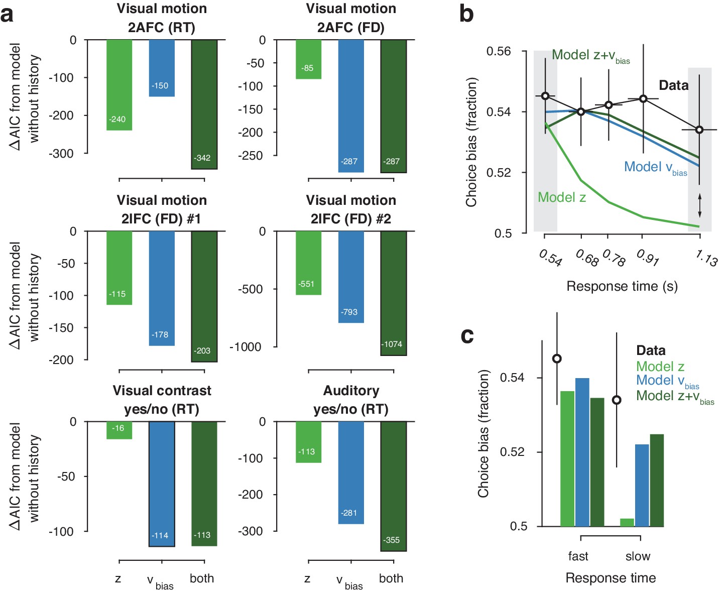
Models with history-dependent biases better explained the data than the baseline model without such history dependence (Figure 3a), corroborating the observation that observers’ behavior showed considerable dependence on previous choices (Figure 2f). The model with both history-dependent starting point and drift bias provided the best fit to five out of six datasets (Figure 3a), based on the Akaike Information Criterion (AIC; Akaike, 1974 - note that we obtained the same results when instead using the hierarchical Deviance Information Criterion).

Figure 3 with 2 supplements see all

Download asset Open asset

Model comparison and simulations.

(a) For each dataset, we compared the AIC between models where drift bias, starting point bias or both were allowed to vary as a function of previous choice. The AIC for a model without history dependence was used as a baseline for each dataset. Lower AIC values indicate a model that is better able to explain the data, taking into account the model complexity; a ΔAIC of 10 is generally taken as a threshold for considering one model a sufficiently better fit. (b) Conditional bias functions (Figure 1c; White and Poldrack, 2014). For the history-dependent starting point, drift bias and hybrid models, as well as the observed data, we divided all trials into five quantiles of the RT distribution. Within each quantile, the fraction of choices in the direction of an individual’s history bias (repetition or alternation) indicates the degree of choice history bias. Error bars indicate mean ± s.e.m. across datasets. (c) Choice bias on slow response trials can be captured only by models that include history-dependent drift bias. Black error bars indicate mean ± s.e.m. across datasets, bars indicate the predicted fraction of choices in the first and last RT quantiles.

https://doi.org/10.7554/eLife.46331.004

The above model comparison pointed to the importance of including a history-dependency into the model. We further examined the ability of each model to explain specific diagnostic features in the data (Palminteri et al., 2017) that distinguished starting point from drift bias. A history-dependent shift in the starting point leads to biased choices primarily when responses are fast (early RT quantiles), whereas a history-dependent shift in drift leads to biased choices across all trials, including those with slow responses (Figure 1). We simulated choices and RTs from the three different model variants and computed so-called ‘conditional bias functions’ (White and Poldrack, 2014): the fraction of choices in line with each observer’s choice repetition tendency (i.e. repetition probability), in each quantile of their RT distribution. For observers whose choice repetition probability was >0.5, this was the fraction of repetitions; for the other observers, this was the fraction of alternations. Consistent with a shift in drift bias, observers exhibited history-dependent choice biases across the entire range of RTs (Figure 3b). In particular, the biased choices on slow RTs could only be captured by models that included a history-dependent shift in drift bias (Figure 3c, blue and dark green bars).

We used the parameter estimates obtained from the full model (with both history-dependent starting point and drift bias) to investigate how history-dependent variations in starting point and drift bias related to each individual’s tendency to repeat their previous choices. We call each bias parameter’s dependence on the previous choice its ‘history shift’. For instance, in the left vs. right motion discrimination task, the history shift in starting point was computed as the difference between the starting point estimate for previous ‘left’ and previous ‘right’ choices, irrespective of the category of the current stimulus. The history shift in drift bias, but not the history shift in starting point, was robustly correlated to the individual probability of choice repetition (Figure 4a, significant correlations indicated with solid regression lines). In five out of six datasets, the correlation with the history shift in drift bias was significantly stronger than the correlation with the history shift in starting point (Figure 4b, Δ $ρ$ values).

Figure 4 with 5 supplements see all

Download asset Open asset

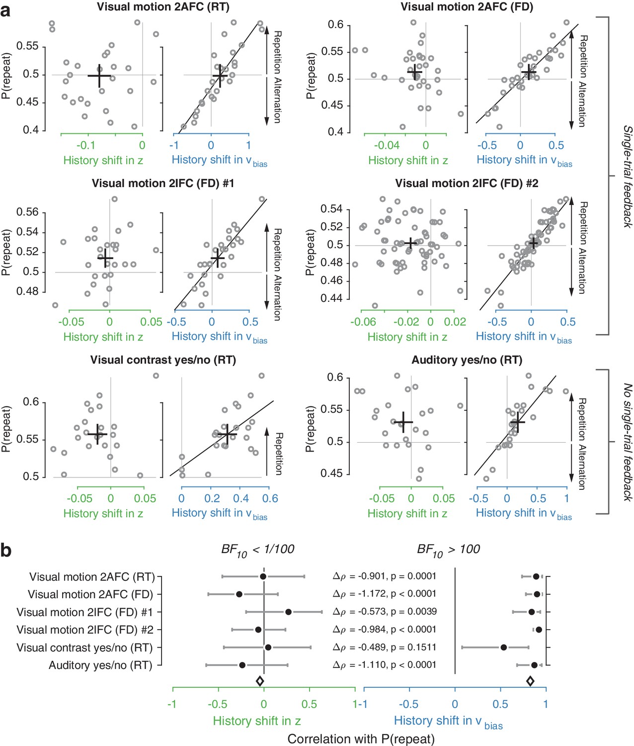
Individual choice history biases are explained by history-dependent changes in drift bias, not starting point.

(a) Relationship between individual choice repetition probabilities, P(repeat), and history shift in starting point (left column, green) and drift bias (right column, blue). Parameter estimates were obtained from a model in which both bias terms were allowed to vary with previous choice. Horizontal and vertical lines, unbiased references. Thick black crosses, group mean ± s.e.m. in both directions. Black lines: best fit of an orthogonal regression (only plotted for correlations significant at p<0.05). (b) Summary of the correlations (Spearman’s ρ) between individual choice repetition probability and the history shifts in starting point (green; left) and drift bias (blue; right). Error bars indicate the 95% confidence interval of the correlation coefficient. Δρ quantifies the degree to which the two DDM parameters are differentially able to predict individual choice repetition (p-values from Steiger’s test). The black diamond indicates the mean correlation coefficient across datasets. The Bayes factor (BF₁₀) quantifies the relative evidence for the alternative over the null hypothesis, with values < 1 indicating evidence for the null hypothesis of no correlation, and >1 indicating evidence for a correlation.

https://doi.org/10.7554/eLife.46331.007

We quantified the total evidence by computing a Bayes factor for each correlation (Wetzels and Wagenmakers, 2012), and multiplying these across datasets (Scheibehenne et al., 2016). This further confirmed that individual choice history biases were not captured by history shifts in starting point, but consistently captured by history shifts in drift (Figure 4b). Specifically, the Bayes factor for the history shift in starting point approached zero, indicating strong evidence for the null hypothesis of no correlation. The Bayes factor for the history shift in drift indicated strong evidence for a correlation (Kass and Raftery, 1995).

Correlations between estimated history shifts in starting point and drift bias were generally negative (mean $ρ$ : −0.2884, range −0.4130 to −0.0757), but reached statistical significance (p<0.05) in only one dataset. The combined Bayes Factor (BF₁₀) was 0.0473, indicating strong evidence for H₀. We thus remain agnostic about the relationship between the history shifts of both parameters.

The same qualitative pattern of results was obtained with an alternative fitting procedure (non-hierarchical G² optimization, Figure 4—figure supplement 2a), as well as a model that allowed for additional across-trial variability in non-decision time (Figure 4—figure supplement 2b). Letting non-decision time vary with each level of sensory evidence strength (in the two datasets including multiple such levels) did not change the pattern of model comparison and correlation results (Figure 4—figure supplement 2c). These findings are thus robust to specifics of the model and fitting method. The Visual motion 2IFC #2 also included pharmacological interventions in two sub-groups of participants (see Materials and methods); we found the same effects for both drug groups as well as the placebo group (Figure 4—figure supplement 3). A significant positive correlation between history shift in drift bias and P(repeat) was present for two sub-groups of participants, defined as ‘repeaters’ and ‘alternators’ (based on P(repeat) being larger or smaller than 0.5, respectively; Figure 4—figure supplement 4).

The lack of a correlation between history-dependent starting point shifts and individual choice repetition is surprising in light of previous accounts (Yu and Cohen, 2008; Gao et al., 2009). History shifts in starting point were mostly negative (a tendency toward choice alternation) across participants, regardless of their individual tendency toward choice repetition or alternation (Figure 4—figure supplement 5, significant in two out of six datasets). This small but consistent effect likely explains why our formal model comparison favored a model with both history-dependent drift and starting point over one with only drift bias (see also Discussion). Critically, only the history-dependent shift in drift bias accounted for individual differences in choice repetition (Figure 4).

History-dependent accumulation bias explains individual choice repetition behavior irrespective of previous choice outcome

In four out of six tasks, participants received explicit outcome feedback (correct, error) after each choice. It is possible that participants experienced positive feedback as rewarding and (erroneously) assumed that a rewarded choice is more likely to be rewarded on the next trial. Manipulations of reward (probability or magnitude) have been found to change starting point (Voss et al., 2008; Leite and Ratcliff, 2011; Mulder et al., 2012), but might also bias drift (Liston and Stone, 2008; Afacan-Seref et al., 2018; Fan et al., 2018). Given that there were far more correct (i.e. rewarded) choices than errors, the history-dependent drift bias could reflect the expectation of reward for the choice that was correct on the previous trial.

Two findings refute this idea. First, the same result holds in the two datasets without single-trial outcome feedback (Figure 4a, bottom row), implying that external feedback is not necessary for history shifts in drift bias. Second, we found similar results when separately estimating the model parameters (history shift in starting point and drift bias) and model-free measures (choice repetition probability) after both correct and error trials (Figure 5a). Across datasets, individual repetition probability was best explained by history shifts in drift bias, not starting point, after both correct (Figure 5b) and error (Figure 5c) trials. Thus, even erroneous choices bias evidence accumulation on the next trial, in the same direction as correct choices. Indeed, most participants were predominantly biased by their previous choice (95 ‘stay’, 30 ‘switch’), while a third was biased by a combination of the previous choice and its correctness (26 ‘win-stay lose-switch’, 42 ‘win-switch lose-stay’; Figure 2c).

Figure 5

Download asset Open asset

History shift in drift bias explains individual choice behavior after both error and correct decisions.

As in Figure 4, but separately following correct (black) and error (red) trials. Post-correct trials were randomly subsampled to match the trial numbers of post-error trials. (a) Relationship between repetition probability and history shifts in starting point and drift bias, separately computed for trials following correct (black circles) and error (red squares) responses. (b) Summary of correlations (as in Figure 4c) for trials following a correct response. Error bars indicate the 95% confidence interval of the correlation coefficient. (c) Summary of correlations (as in Figure 4c) for trials following an error response. (d) Difference in correlation coefficient between post-correct and post-error trials, per dataset and parameter. Δρ quantifies the degree to which the two DDM parameters are differentially able to predict individual choice repetition (p-values from Steiger’s test). The black diamond indicates the mean correlation coefficient across datasets. The Bayes factor (BF₁₀) quantifies the relative evidence for the alternative over the null hypothesis, with values < 1 indicating evidence for the null hypothesis of no correlation, and >1 indicating evidence for a correlation.

https://doi.org/10.7554/eLife.46331.013

Correlations tended to be smaller for previous erroneous choices. However, directly comparing the correlation coefficients between post-correct and post-error trials (after subsampling the former to ensure equal trial numbers per participant) did not allow us to refute nor confirm a difference (Figure 5d). In sum, history-dependent drift biases did not require external feedback about choice outcome and were predominantly induced by the previous choice. These choice history-dependent biases in evidence accumulation were accompanied by effects on drift rate and boundary separation (Figure 4—figure supplement 1), in line with previous work on post-error slowing (Dutilh et al., 2012; Goldfarb et al., 2012; Purcell and Kiani, 2016a).

Accumulation bias correlates with several past choices

Does the history shift in evidence accumulation depend on events from one past trial only? Recent work has exposed long-lasting choice history biases that span several trials and tens of seconds (Urai et al., 2017; Braun et al., 2018; Hermoso-Mendizabal et al., 2018). We thus estimated the influence of past events on the evidence accumulation process in a more comprehensive fashion. We fit a family of models in which correct and incorrect choices from up to six previous trials were used as predictors, and estimated their contribution to current starting point and drift bias.

Inclusion of further lags improved the model’s ability to account for the data, up to a lag of 2–4 after which model fits (ΔAIC) began to deteriorate (Figure 6—figure supplement 1). In 4/6 datasets, the best-fitting model contained only history-dependent changes in drift, not starting point, over a scale of the previous 2–4 trials. In the other two datasets, the best-fitting model was a hybrid where both drift and starting point varied as a function of choice history, up to two to trials into the past (Figure 6—figure supplement 1). We computed ‘history kernels’ across the different lags, separately for starting point and drift bias. These are analogous to the kernels obtained from a history-dependent regression analysis of the psychometric function that ignores decision time (Fründ et al., 2014), and which have been widely used in the recent literature on choice history biases (Fründ et al., 2014; Urai et al., 2017; Braun et al., 2018). To interpret these group-level kernels in light of substantial individual variability, we expressed each regression weight with respect to individual repetition probability at lag 1 (i.e. switching the sign for alternators).

Previous choices shifted drift bias in line with individual history bias across several trials, whereas starting point did not consistently shift in the direction of history bias. The hybrid models showed that the effect of choice history on drift bias decayed over approximately three past trials (Figure 6a), with a slower decay than for starting point (Figure 6a). The regression weights for past trials (from lag two through each dataset’s best-fitting lag) for drift bias – but not starting point - significantly correlated with the probability of repeating past choices at these same lags (Figure 6b). This was true after both correct and error trials (Figure 6b), similarly to the effects at lag 1 (Figure 5b–c).

Figure 6 with 1 supplement see all

Download asset Open asset

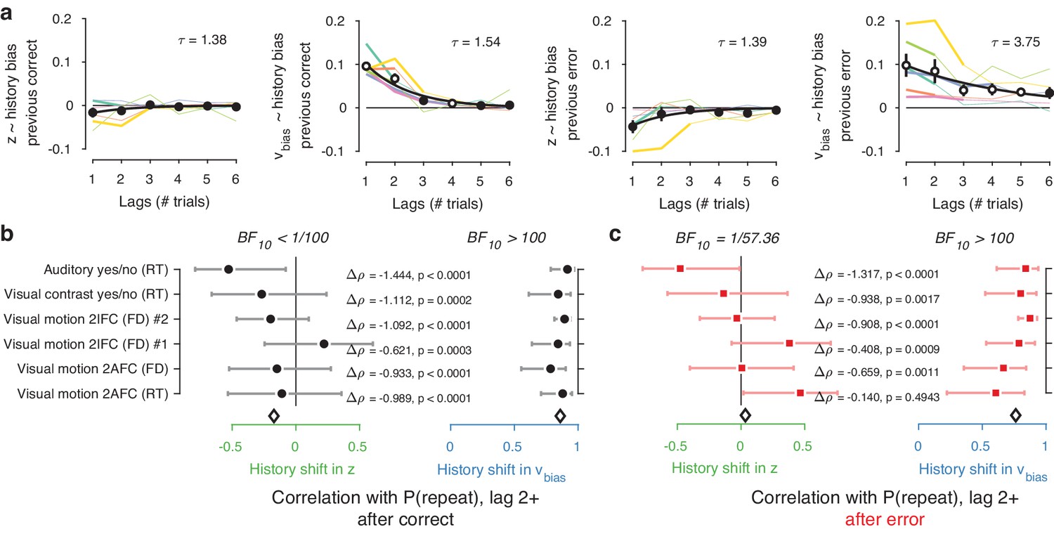
Choice history affects drift bias over multiple trials.

(a) History kernels, indicating different parameters’ tendency to go in the direction of each individual’s history bias (i.e. sign-flipping the parameter estimates for observers with P(repeat)<0.5). For each dataset, regression weights from the best-fitting model (lowest AIC, Figure 6—figure supplement 1) are shown in thicker lines; thin lines show the weights from the largest model we fit. Black errorbars show the mean ± s.e.m. across models, with white markers indicating timepoints at which the weights are significantly different from zero across datasets (p<0.05, FDR corrected). Black lines show an exponential fit $V (t) = A e^{- t / τ}$ to the average. (b) Correlations between individual P(repeat) and regression weights, as in Figure 5b–c. Regression weights for the history shift in starting point and drift bias were averaged from lag two until each dataset’s best-fitting lag. P(repeat) was corrected for expected repetition at longer lags given individual repetition, and averaged from lag two to each dataset’s best-fitting lag. Δρ quantifies the degree to which the two DDM parameters are differentially able to predict individual choice repetition (p-values from Steiger’s test). The black diamond indicates the mean correlation coefficient across datasets. The Bayes factor (BF₁₀) quantifies the relative evidence for the alternative over the null hypothesis, with values < 1 indicating evidence for the null hypothesis of no correlation, and >1 indicating evidence for a correlation.

https://doi.org/10.7554/eLife.46331.014

In sum, the biasing effect of choice history on evidence accumulation is long-lasting (longer than the effects on starting point), dependent on preceding choices several trials into the past, but independent of their correctness. This analysis corroborates the previous findings from our simpler models focusing on only the preceding trial, and further dissociate the effects of choice history on starting point and evidence accumulation.

History-dependent accumulation bias explains individual choice repetition behavior irrespective of specifics of bounded-accumulation models

We next set out to test the generality of our conclusions and gain deeper mechanistic insight into the nature of the dynamic (i.e. time-increasing) bias. We used a variety of bounded-accumulation models with more complex dynamics than the standard DDM. We focused on the preceding trial only, which our previous analyses had identified as exerting the same effect on history bias as the longer lags (Figure 6). These models included variants of the DDM (i.e. a perfect accumulator) with more complex dynamics of the bias or the decision bounds, as well as variants of a leaky accumulator (Busemeyer and Townsend, 1993; Usher and McClelland, 2001; Brunton et al., 2013). We focused on the Visual motion 2AFC (FD) dataset because it entailed small random dot stimuli (diameter 5° of visual angle), leading to large within- and across-trial fluctuations in the sensory evidence which we estimated through motion energy filtering (Adelson and Bergen, 1985; Urai and Wimmer, 2016; Figure 7—figure supplement 1). These fluctuating motion energy estimates were used as time-varying sensory input to the models, providing key additional constraints over and above nominal sensory evidence levels, choices and RT distributions (Brunton et al., 2013).

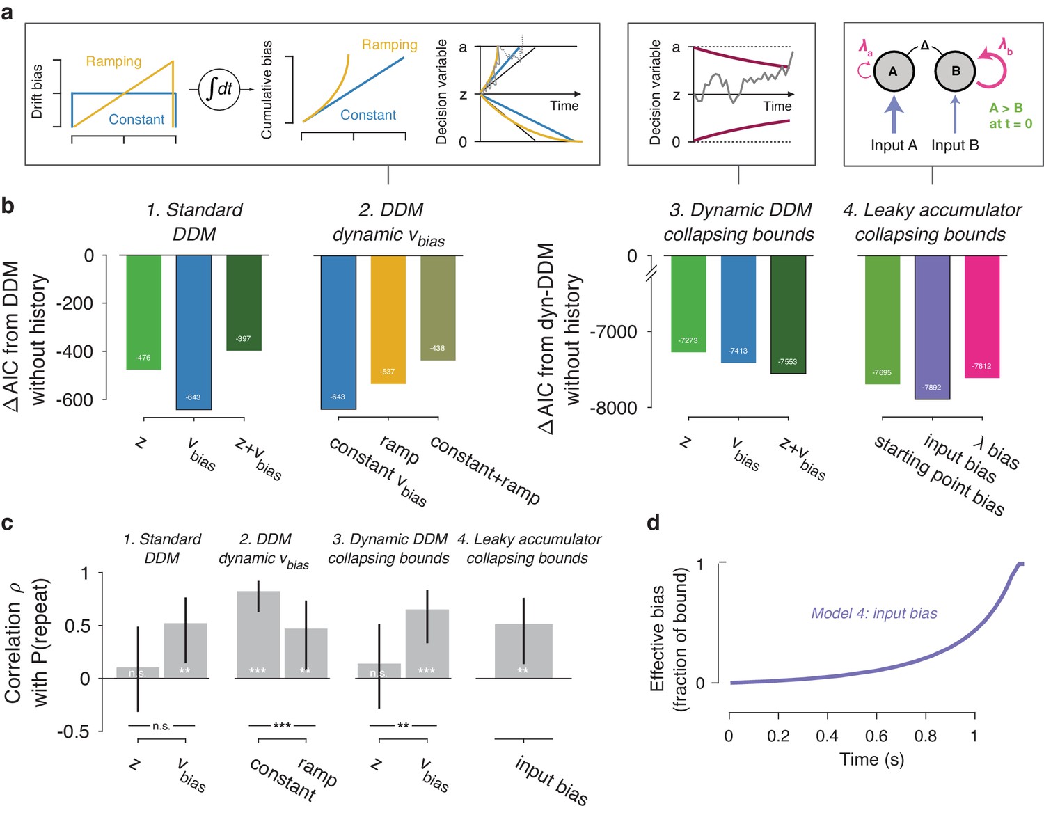
We first re-fit the standard DDM where the two biasing parameters were allowed to vary with previous choice (see Figure 1), now using single-trial motion energy estimates and a non-hierarchical fitting procedure (see Materials and methods). This made these fits directly comparable to both the hierarchical fits in Figures 3–4, and the more complex models described below. As expected (Figure 3a), the data were better explained by a history-dependent bias in the drift, rather than the starting point (Figure 7b1). In these non-hierarchical fits, the hybrid DDM (i.e. both bias terms free to vary as a function of previous choice) lost against the drift bias-only model (indicated by its higher AIC). Yet thi hybrid model allowed for a direct comparison of the correlations between these (jointly fit) bias parameters and individual choice repetition probability. As in our previous analysis (Figure 4), individual choice repetition probability was more strongly predicted by drift than starting point bias (Figure 6c1).

Figure 7 with 3 supplements see all

Download asset Open asset

Extended dynamic models of biased evidence accumulation.

(a) Model schematics. In the third panel from the left, the stimulus-dependent mean drift is shown in black, overlaid by the biased mean drift in color (as in Figure 1a,b). (b) AIC values for each history-dependent model, as compared to a standard (left) or dynamic (right) DDM without history. The winning model (lowest AIC value) within each model class is shown with a black outline. (c) Correlation (Spearman’s ρ) of parameter estimates with individual repetition behavior, as in Figure 4b. Error bars, 95% confidence interval. ***p<0.0001, **p<0.01, n.s. p>0.05. (d) Within-trial time courses of effective bias (cumulative bias as a fraction of the decision bound) for the winning leaky accumulator model. Effective bias time courses are indistinguishable between both dynamical regimes (λ < 0 and λ > 0) and are averaged here.

https://doi.org/10.7554/eLife.46331.016

A previous study of reward effects on speeded decisions reported that reward asymmetries induced supra-linear bias dynamics (Afacan-Seref et al., 2018). Temporal integration of a constant drift bias produces a linearly growing effective bias in the decision variable (Figure 1b), whereas integration of a ramping drift bias produces a supra-linear growth of effective bias (Figure 7a, yellow). In our data, a standard DDM with constant drift bias provided a better fit than DDMs with either a ramping drift bias, or a combination of constant and ramping drift bias (Figure 7b2). Furthermore, in the latter (hybrid) model, the constant drift bias best predicted individual choice repetition behavior (Figure 7c2), in line with the constant accumulation bias inferred from the standard DDM fits. For the fits shown in Figure 7b2/c2, we used the same fitting protocol as for the standard DDM, in which the time-varying sensory evidence fluctuations during stimulus presentation were replaced by their average over time to compute a single-trial drift rate (called ‘default protocol’, Materials and methods section Extended bounded accumulation models: General assumptions and procedures). The same qualitative pattern of results also held for another fitting protocol (‘dynamic protocol’, see Materials and methods), in which the time-varying sensory evidence was fed into the integrator (ΔAIC relative to no-history model: −1103, –985, −995, for constant drift bias, ramping drift bias, and hybrid, respectively; correlation with P(repeat): ρ(30)= 0.5458, p=0.0012; ρ(30)= 0.3600, p=0.0429 for constant and ramping drift bias, respectively). We next used this dynamic protocol for a set of more complex dynamical models.

It has been proposed that decision bounds might collapse over time, implementing an ‘urgency signal’ (Figure 6a, middle; Churchland et al., 2008; Cisek et al., 2009). Indeed, adding collapsing bounds substantially improved our model fits (Figure 7b3). This indicates the presence of a strong urgency signal in this task, which had a relatively short stimulus presentation (750 ms) and a tight response deadline (1.25 s after stimulus offset). Critically, a history-dependent drift bias best fit the data (Figure 7b3) and captured individual choice repetition behavior (Figure 7c3) also in the DDM with collapsing bounds. In other words, while there is evidence for collapsing bounds in this dataset, our conclusion about the impact of history bias on decision formation does not depend on its inclusion in the model.

In the brain, a neural representation of the momentary sensory evidence feeds into a set of accumulators. These consist of circuits of excitatory and inhibitory populations of cortical neurons, which give rise to persistent activity and competitive winner-take-all dynamics (Usher and McClelland, 2001; Wang, 2002). Under certain parameter regimes, these circuit dynamics can be reduced to lower-dimensional models (Bogacz et al., 2006; Wong, 2006). In such models, the effective accumulation time constant 1/λ (with λ being the effective leak) results from the balance of leak within each accumulator (due to self-excitation and passive decay) and mutual inhibition between two accumulators encoding different choices (Usher and McClelland, 2001). Evidence accumulation can then be biased through an internal representation of the sensory input, or through the way this sensory representation is accumulated (Figure 7a, right). We here used a reduced competing accumulator model, where the decision variable was computed as the difference of two leaky accumulators (Busemeyer and Townsend, 1993; Zhang and Bogacz, 2010; see also Brunton et al., 2013) to compare these two accumulation biases and a biased accumulator starting point.

We fit a family of bounded, leaky accumulator models, in which the starting point of the accumulators, their input, or their effective leak λ could be biased as a function of previous choice (Figure 7a, right). Note that a bias of the accumulator starting point would also translate into an accumulation bias, due to the model dynamics (see Materials and methods section Extended bounded accumulation models: General assumptions and procedures). Even so, comparing this regime with other two biasing mechanism was informative. Also note that we here use the term ‘leaky accumulator model’ to denote that the model dynamics consisted of a free effective leak parameter λ, without implying that λ < 0 (corresponding to activation decay). Our fits allowed λ to take either negative (‘forgetful’ regime) or positive (‘unstable’ regime) values (Figure 7—figure supplement 1d; see also Brunton et al., 2013). Critically, in order to test for choice history-dependent accumulation bias, we allowed λ of each accumulator to vary as a function of the previous choice, before computing the difference between the two accumulator activations. Choice-history dependent biases in accumulator starting point or accumulator input were directly applied to the accumulator difference (akin to starting point and drift bias within the DDM). Due to the simplicity of its dynamics, the DDM cannot distinguish between input and leak bias. Indeed, when simulating behavior of leaky accumulator models with either of these two accumulation biases and fitting it with the DDM, both input and λ bias loaded onto DDM drift bias (Figure 7—figure supplement 2). Critically, the leaky accumulator with biased accumulator input best explained the data, among all the models considered (Figure 7b4). Furthermore, the individually estimated input bias predicted individual choice repetition (Figure 7c4). This suggests that choice history might specifically bias the internal representation of sensory evidence feeding into the evidence accumulation process.

Dynamics of effective bias signal approximates rational combination of prior information with current evidence

Taken together, fits and simulations of more complex models provided additional insight into the mechanism underlying choice history bias. They also corroborated the conclusion that choice history biases are mediated by a biased accumulation of evidence, rather than a biased starting point. As a final step, we estimated the time course of the effective bias, computed as the fraction of cumulative bias signal and bound height (Hanks et al., 2011). We simulated this signal based on the group average parameters for the best-fitting leaky accumulator model (Figure 7d). In this leaky accumulator (with collapsing bound), the effective bias accelerated (Figure 7d).

The reader may notice that these (supra-linear) effective bias dynamics are similar to those predicted by the DDM with a ramping drift bias (Figure 7a, left). Thus, the observation that the latter model lost by a wide margin against the two models with more complex dynamics (Figure 7b, see also Materials and methods) is likely due to features of the data other than the (relatively small) selective history bias. Specifically, the RT distributions were strongly shaped by the urgency signal incorporated by the bound collapse. In the overall best-fitting model (leaky accumulator with collapsing bounds and input bias, Figure 7b5), this effective bias depends on the combined effect of two non-linear signals: (i) the cumulative bias resulting from the accumulation of biased input and (ii) the hyperbolically collapsing bound. In the current fits, the effective bias was dominated by the strong bound collapse, but in different circumstances (with weaker urgency signal and for λ < 0), a biased input leaky accumulator can produce a decelerating effective bias. Combination of a biased input with some starting point and or leak bias can further change the dynamics. The key observation is that, regardless of the modeling framework used, we identified an effective bias signal that grew steadily throughout decision formation, in line with the main conclusion drawn from the basic fits of the standard DDM.

Our results are in line with the idea the impact of choice history bias on decision formation grows as a function of elapsed time. This observation might be surprising, as prior information (here: about the previous choice) does not change over time. Yet, previous work has identified a principled rationale for such a time-dependent combination of prior and evidence. When evidence reliability changes from trial to trial, prior information (bias) should be weighted more strongly when sensory evidence is unreliable (Hanks et al., 2011; Moran, 2015). This can be achieved by increasing the weight of the prior throughout the trial, using elapsed time as a proxy for evidence reliability. This prediction was confirmed experimentally for explicit manipulations of prior probability of the choice options (Hanks et al., 2011). Indeed, within the framework of the DDM, this way of combining prior information with current evidence maximizes reward rate (Moran, 2015; see also Drugowitsch and Pouget, 2018). Only when evidence reliability is constant across trials should prior information be incorporated as a static bias (i.e. starting point). Evidence reliability likely varied from trial to trial across all our experiments (Moran, 2015), due to variations in the external input (i.e. mean drift rate in the DDM), originating from stochastically generated stimuli, or internal factors (i.e. drift rate variability in the DDM), such as the inherent variability of sensory cortical responses (Arieli et al., 1996; Faisal et al., 2008). In particular, the dataset from Figure 7 entailed strong trial-to-trial variations in the external input (Figure 7—figure supplement 1). Thus, the dynamics of the effective bias signal uncovered in Figure 7d suggest that participants combined prior information with current evidence in a rational fashion.

Discussion

Quantitative treatments of perceptual decision-making commonly attribute trial-to-trial variability of overt choices to noisy decision computations (Shadlen et al., 1996; Renart and Machens, 2014; Wyart and Koechlin, 2016). Those accounts typically assume that systematic decision biases remain constant over time. Instead, the choice history biases studied here vary continuously over the course of the experiment, as a function of the previous choices (and choice outcome information). Our current results indicate that choice history explains trial-to-trial variability specifically in evidence accumulation, in a number of widely used perceptual choice tasks. Ignoring such trial-to-trial variations will lead to an overestimation of the noise in the evidence accumulation process and resulting behavior.

History biases in perceptual choice have long been known in perceptual psychophysics (Fernberger, 1920) and neuroscience (Gold et al., 2008). However, the underlying dynamic mechanisms have remained elusive. We here show that individual differences in overt choice repetition behavior are explained by the degree to which choices bias the evidence accumulation, not the starting point, of subsequent decisions. This accumulation bias is associated with choices made several trials into the past, and it grows steadily as the current decision unfolds. This insight calls for a revision of current models of choice history biases (Yu and Cohen, 2008; Zhang et al., 2014).

It is instructive to relate our results to previous studies manipulating the probability of the occurrence of a particular category (i.e. independently of the sequence of categories) or the asymmetry between rewards for both choices. Most of these studies explained the resulting behavioral biases in terms of starting point shifts (Leite and Ratcliff, 2011; Mulder et al., 2012; White and Poldrack, 2014; Rorie et al., 2010; Gao et al., 2011; but only for decisions without time pressure, see Afacan-Seref et al., 2018). Yet, one study with variations of evidence strength found an effect of asymmetric target probability on accumulation bias (Hanks et al., 2011) similar to the one we here identified for choice history. In all this previous work, biases were under experimental control: probability or reward manipulations were signaled via explicit task instructions or single-trial cues (in humans) or block structure (in animals). By contrast, the choice history biases we studied here emerge spontaneously and in an idiosyncratic fashion (Figure 2e), necessitating our focus on individual differences.

Our modeling addressed the question of how prior information is combined with new evidence during decision formation (see in particular the section Dynamics of effective bias signal approximates rational combination of prior information with current evidence). But why did participants use choice history as a prior for their decisions? In all our experiments, the sensory evidence was uncorrelated across trials – as is the case in the majority of perceptual choice tasks used in the literature. Thus, any history bias can only reduce performance below the level that could be achieved, given the observer’s sensitivity. It may seem irrational that people use history biases in such settings. However, real-world sensory evidence is typically stable (i.e. auto-correlated) across various timescales (Yu and Cohen, 2008). Thus, people might (erroneously) apply an internal model of this environmental stability to randomized laboratory experiments (Yu and Cohen, 2008), which will push them toward choice repetition or alternation (Glaze et al., 2015). Indeed, people flexibly adjust their choice history biases to environments with different levels of stability (Glaze et al., 2015; Kim et al., 2017; Braun et al., 2018), revealing the importance of such internal models on perceptual decision-making. In sum, with our conclusions from the time course of the effective bias signal, these considerations suggest that participants may have applied a rational strategy, but based on erroneous assumptions about the structure of the environment.

While we found that choice history-dependent variations of accumulation bias were generally more predictive of individual choice repetition behavior, the DDM starting point was consistently shifted away from the previous response for a majority of participants (i.e. negative values along x-axis of Figure 4a). This shift was statistically significant in three out or six datasets (Figure 4—figure supplement 5a), and might explain the advantage of the dual parameter model over the pure drift-bias model in our model comparisons (Figure 3a). The starting point shift may be due to at least two scenarios, which are not mutually exclusive. First, it might reflect a stereotypical response alternation tendency originating from neural dynamics in motor cortex – for example, a post-movement ‘rebound’ of beta-band oscillations (Pfurtscheller et al., 1996). Indeed, previous work found that beta rebound is related to response alternation in a perceptual choice task, which precluded (in contrast to our tasks) motor planning during evidence accumulation (Pape and Siegel, 2016). This stereotypical response alternation tendency (via starting point) may have conspired with the more flexible history bias of evidence accumulation (via drift bias) to shape choice behavior. Because starting point shifts will predominantly contribute to fast decisions, this scenario is consistent with the average choice alternation tendency we observed for RTs < 600 ms (Figure 4—figure supplement 5c). Because the response alternation tendency in motor cortex is likely to be induced only by the immediately preceding response, this scenario is also consistent with the shorter timescales we estimated for the starting point effects (1.39 trials) than the drift rate effects (2.38 trials; Figure 6a, exponential fits). Second, the starting point shift may also reflect decision dynamics more complex than described by the standard DDM: non-linear drift biases (Figure 7—figure supplement 2, third column) or biases in the leak of decision accumulators (Figure 7—figure supplement 3, third column). Both give rise to opposite effects on drift bias and starting point bias when fit with the standard DDM, thus yielding negative correlations between DDM starting point and drift bias estimates. Such negative correlations were present in our data, but weak and not statistically significant (Spearman’s rho −0.4130 to −0.0757, combined BF₁₀= 0.0473). It is possible that both of the scenarios discussed here conspired to yield the starting point effects observed in model comparisons and individual parameter estimates. Future work is needed to illuminate this issue, for example through manipulating decision speed and/or the delays between subsequent motor responses, and modeling choice-related neural dynamics in motor cortex.

We propose that choice history biases evidence accumulation, but there are alternative scenarios. First, it is possible that participants’ choices were due to computations altogether different from those incorporated in the bounded accumulation models assessed here. All our models imply simple neural accumulators with persistent activity. At least on a subset of trials, participants may make fast guesses (Noorbaloochi et al., 2015), or engage in automatic decision processing (Servant et al., 2014; Ulrich et al., 2015) or post-accumulation biases (Erlich et al., 2015). The decision computation may also entail noise-driven attractor dynamics (Wang, 2002; Braun and Mattia, 2010) possibly with sudden ‘jumps’ between neural activity states (Latimer et al., 2015), instead of linear accumulation to a threshold level. Even if the accumulation dynamics postulated in our models cannot be reduced to the dynamics of single neurons, the history-dependent accumulation bias we inferred here would constitute a valid description of the collective computational properties of the neural system producing choice behavior. Second, within bounded accumulation models, any directed change in the decision variable can be mimicked by some selective (i.e. asymmetric) change in one of the decision bounds. For example, combining the DDM with a linearly collapsing bound for the favored choice and a linearly expanding bound for the other choice has the same effect on choice fractions and RT distributions as a drift bias. We are not aware of any empirical evidence for such asymmetric changes in decision bounds. Decision-related cortical ramping activity seems to always reach a fixed level just before motor response, irrespective of prior probabilities (Hanks et al., 2011) or speed-accuracy trade-offs (Hanks et al., 2014; Murphy et al., 2016). Instead, the build-up of this activity is biased by prior information (Hanks et al., 2011).

A plausible mechanism underlying the choice history-dependent shift in accumulation bias is a bias of the neural representations of the sensory evidence towards (or away from) a previously selected category (Nienborg and Cumming, 2009; St John-Saaltink et al., 2016; Urai and Wimmer, 2016). This is precisely the ‘input bias’ scenario entailed in our best fitting model (Figure 7). The primate brain is equipped with powerful machinery to bias sensory representations in a top-down fashion (Desimone and Duncan, 1995; Reynolds and Heeger, 2009). In the laboratory, these top-down mechanisms have been probed by explicitly instructing subjects to shift their attention to a particular sensory feature or location. Such instructions induce biased activity states in regions of prefrontal and parietal association cortex, which are propagated down the cortical hierarchy to sensory cortex via selective feedback projections, where they boost the corresponding feature representations and suppress others (Desimone and Duncan, 1995). The same prefrontal and parietal regions accumulate sensory evidence and seem to carry choice history signals. It is tempting to speculate that choice history signals in these regions cause the same top-down modulation of sensory cortex as during explicit manipulations of attention. In other words, agents’ choices might be one factor directing their top-down attention under natural conditions, in a way analogous to explicit attention cues in laboratory tasks. An alternative, but related possibility is that the direction of selective attention fluctuates spontaneously during the course of a perceptual choice experiment, preferentially sampling features supporting one choice for a streak of trials, and then switching to sampling support for the other category. The corresponding top-down modulations would bias evidence accumulation and choice in a serially correlated fashion. These ideas are not mutually exclusive and can be tested by means of multi-area neurophysiological recordings combined with local perturbations.

A growing body of evidence points to the interplay of multiple timescales for neural computation in the cortex. One line of behavioral work has revealed effective (within-trial) evidence accumulation over timescales ranging from a few hundred milliseconds (Kiani et al., 2008; Tsetsos et al., 2015) to several seconds (Tsetsos et al., 2012; Wyart et al., 2012; Cheadle et al., 2014). Another line of work, including the current study, revealed the slow accumulation of internal decision variables or external outcome information across trials (tens of seconds) to build up time-varying biases, or priors (Sugrue et al., 2004; Abrahamyan et al., 2016; Purcell and Kiani, 2016b; Braun et al., 2018). Relatedly, neurophysiological work on ongoing activity has inferred multiple hierarchically organized timescales in different cortical regions (Honey et al., 2012; Murray et al., 2014; Chaudhuri et al., 2015; Runyan et al., 2017; Scott et al., 2017). The history-dependent evidence accumulation biases that we have uncovered here might index the interplay between these different effective timescales, with long-timescale accumulators at higher stages biasing short-timescale accumulators at intermediate stages of the cortical hierarchy.

Share this article

Cite this article

Two biasing mechanisms within the DDM.

Behavioral tasks and individual differences.

Model comparison and simulations.

Individual choice history biases are explained by history-dependent changes in drift bias, not starting point.

History shift in drift bias explains individual choice behavior after both error and correct decisions.

Choice history affects drift bias over multiple trials.

Extended dynamic models of biased evidence accumulation.

Author details

Anne E Urai

Present address

Contribution

For correspondence

Competing interests

Jan Willem de Gee

Present address

Contribution

Competing interests

Konstantinos Tsetsos

Contribution

Contributed equally with

Competing interests

Tobias H Donner

Contribution

Contributed equally with

For correspondence

Competing interests

Downloads (link to download the article as PDF)

Open citations (links to open the citations from this article in various online reference manager services)

Cite this article (links to download the citations from this article in formats compatible with various reference manager tools)

Categories and tags

Research organism

Further reading