

Abstract
The distribution of in vivo average firing rates within local cortical networks has been reported to be highly skewed and long tailed. The distribution of average single-cell inputs, conversely, is expected to be Gaussian by the central limit theorem. This raises the issue of how a skewed distribution of firing rates might result from a symmetric distribution of inputs. We argue that skewed rate distributions are a signature of the nonlinearity of the in vivo f–I curve. During in vivo conditions, ongoing synaptic activity produces significant fluctuations in the membrane potential of neurons, resulting in an expansive nonlinearity of the f–I curve for low and moderate inputs. Here, we investigate the effects of single-cell and network parameters on the shape of the f–I curve and, by extension, on the distribution of firing rates in randomly connected networks.
Introduction
Since the first in vivo electrophysiological investigations of cortical spiking activity, two general, co-occurring features have been reported ubiquitously. Single-cell spike trains are far from being regular, as those one would obtain in vitro by injecting constant currents; rather, they resemble those that would be generated by a Poisson-like process (Softky and Koch 1993; Compte et al., 2003). In addition, time-averaged firing rates of cells recorded in the same area span a wide interval, ranging from <1 Hz up to several tens of hertz (Griffith and Horn, 1966; Koch and Fuster, 1989). The distribution of average firing rates, in various cortical areas and during spontaneous and stimulus-evoked activity, is typically non-Gaussian and significantly long tailed (Shafi et al., 2007; Hromádka et al., 2008; O'Connor et al., 2010).
Theoretical studies of networks of randomly connected spiking neurons have shown that highly irregular spiking activity occurs when a network operates in the fluctuation-driven regimen, i.e., when mean inputs are subthreshold and spiking occurs as a result of fluctuations (van Vreeswijk and Sompolinsky, 1996, 1998; Amit and Brunel, 1997a). These studies have also shown that networks operating in this regimen typically exhibit right-skewed, long-tailed distributions of average firing rates. More recent work showed that similar rate distributions also arise in networks with more structured synaptic connectivity (Amit and Mongillo, 2003; van Vreeswijk and Sompolinsky, 2005; Roudi and Latham, 2007). In short, years of modeling work suggest that a broad, skewed distribution of firing rates is a generic, and robust, feature of spiking networks operating in the fluctuation-driven regimen. A detailed investigation of the factors controlling the shape of the rate distribution is, however, still lacking. We provide here such a study.
We start by characterizing the features of the single-cell f–I curve that control the skewness of the resulting rate distribution. Then, by using networks of leaky integrate-and-fire (LIF) neurons, we study the dependence of those features on single-cell and network parameters. Finally, we perform numerical simulations of networks of Hodgkin–Huxley-type conductance-based neurons to probe the robustness of the proposed mechanism. In all cases, we compare with a lognormal distribution of firing rates, as reported recently by Hromádka et al. (2008).
Materials and Methods
Evaluating the firing rate distribution.
We consider a large population of N neurons (i = 1, …, N) for which the rate νi of neuron i is determined by the transfer function, or f–I curve, νi = ϕ(μi), where the time-averaged input, μi, is drawn from a distribution f(μ). The firing rate distribution, P(ν) of the population is given by
 where δ(x) is the Dirac delta function. This integral can be evaluated explicitly by performing the change of variables w = ϕ(z), and so dw = ϕ′(ϕ−1(w))dz. Finally, this gives

 where the functions ϕ−1 and ϕ′ are the inverse and first derivative of the single-cell f–I curve, ϕ, respectively.
In particular, if the input distribution is Gaussian with mean μ̄ and SD Δ, this can be written as
 From this equation, it is clear that only a linear f–I curve yields a Gaussian firing rate distribution. Writing ϕ(μ) = Aμ + B, leads to
 which is a Gaussian distribution with mean Aμ̄ + B and SD AΔ.
If the transfer function is exponential, ϕ(μ) = ν0eγμ, ϕ−1(ν) = γ−1 log(ν/ν0) and ϕ′(ϕ−1(ν)) = γν. Therefore, we can rewrite Equation 4 as
 which is a lognormal distribution where log(v0) + γ μ̄ and γ2Δ2 are the mean and variance of the logarithm of ν.
The distribution of firing rates can also be easily derived in the case of a power-law transfer function ϕ(μ) = ν0(μ/μ0)ζ, where μ > 0. For such a transfer function, we have ϕ−1(ν) = μ0(ν/ν0)1/ζ and ϕ′(ϕ−1(ν)) = ζν 01/ζ ν1 − 1/ζ/μ0, so that

 where Σ = ζν01/ζ Δ/μ0 and H(ν), δ(ν), and erf(x) are the Heaviside, Dirac delta functions, and error functions, respectively. The delta function takes into account those neurons that have zero firing rate.
In the large ζ limit, using limz→0(xz − 1)/z = ln(x), we can write the rate distribution as
 where M =
Randomly connected network of integrate-and-fire neurons.
We consider a randomly connected network of NE excitatory and NI inhibitory integrate-and-fire neurons. The membrane voltage of the ith neuron of population α = {E, I} obeys the differential equation
 where the parameters τa and Eα are the membrane time constant and resting potential of cells in population α, respectively. Equation 10 is solved together with the reset condition
 where θa is the neuronal threshold, and Vrα is the reset potential. The time t+ indicates that the neuron is reset just after reaching threshold.
The synaptic input, Isyn,iα(t) = Irec,iα(t) + Iext,iα(t), has both a recurrent and an external component. The recurrent connectivity is generated by allowing for a connection from neuron j in population β to a neuron i in population α with a probability p. Thus, we assume an identical connection probability for all four connectivities: E → E, E → I, I → E, I → I. External inputs are modeled as independent Poisson processes. The resulting inputs can be expressed as

 where cijαβ (i = 1, …, Nα, j = 1, …, Nβ) is the connectivity matrix, cijαβ = 1 with probability p, cijαβ = 0 otherwise. Jαβ is the strength of existing synaptic connections, tjk is the kth spike time of neuron j, Dijαβ is the synaptic delay of the connection from neuron j to neuron i, Jα,ext is the strength of the external synaptic connections to neurons of population α, and Ci,extα is the number of external connections of neuron i. External inputs are independently chosen for each neuron, i.e., there is no shared external input between neurons. In Equation 12, the kth action potential of neuron j in population β at time tjk causes a jump of magnitude Jαβ in the membrane voltage of neuron i at a time tjk + Dijαβ if the two neurons are connected (cijαβ = 1). The sum in Equation 12 is therefore over presynaptic neurons and over all action potentials of each presynaptic neuron, respectively. The external input to cell i in population α consists of Ci,extα excitatory presynaptic cells, the activity of which is assumed Poisson with a rate νa,ext. Note that the number of external inputs may vary from cell to cell, hence, the subscript i in Ci,extα. Equations 10–13 are solved together with the reset condition.
Distribution of firing rates in asynchronous states in randomly connected networks of integrate-and-fire neurons.
We analyzed Equations 10 and 11 to determine the distribution of firing rates across neurons and compare it with that found during spontaneous cortical activity in vivo. As such, we choose to study the network in the asynchronous regimen in which single-cell firing is highly irregular. Here we briefly outline this analysis. For a more detailed description, see Amit and Brunel (1997a).
In the asynchronous regimen, the model cells fire approximately as Poisson processes. The input to each cell is therefore a sum over a large number of inputs with approximately Poisson statistics, which, for small values of the connection probability p, are nearly independent. If, furthermore, the individual postsynaptic currents are sufficiently small in amplitude compared with the rheobase, the input current can be cast as a mean input plus a fluctuation term that is delta correlated in time (white noise) and is approximately Gaussian distributed. Because we are interested in spontaneous and therefore stationary activity, we consider only the equilibrium state of the network. The input current is then
 where μ̄α is the mean input averaged in time and over all neurons in population α. The time-averaged mean input for an individual neuron deviates from the population mean because of the quenched randomness in the connectivity. The SD of this quenched variability is given by Da, and zi is an approximately Gaussian distributed random variable with mean zero and unit variance, i.e., zi ϵ N(0,1). The third term in Equation 14 represents temporal fluctuations, which are approximated as Gaussian white noise with amplitude σa, and thus ξi(t) is a Gaussian distributed random variable with zero mean and unit variance and is delta correlated in time. The population mean, population variance, and temporal variance are given by


 where Cα = pNα, Cext is the average number of external connections per cell, and v̄α is the mean firing rate in population α. The quenched variance in mean firing rates, synaptic efficacies, and the number of external inputs to population α are given by Dva2, ΔJα2, and ΔC2, respectively. The equation for the quenched variability in inputs (Eq. 16) has four contributions: variability in the number of recurrent inputs per cell, variability in the presynaptic firing rates, variability in synaptic efficacies, and variability in the number of external inputs per cell, respectively.
Inserting Equation 14 into Equation 10 leads to a Langevin equation. The evolution of the distribution of membrane potentials is therefore given by a Fokker–Planck equation. The mean firing rates vα(z) (α ϵ {E, I}) are determined self-consistently through appropriate boundary conditions of the Fokker–Planck equation, yielding

 The mean and variance of the resulting firing rate distribution are

 Equations 15–21 must be solved self-consistently to obtain the mean and variance of the firing rate distribution for a given set of parameter values. Once this has been done, the distribution of mean firing rates in population α is then
 Note that the distribution of firing rates in a network of randomly connected LIF neurons with conductance-based synapses can be calculated in an analogous way (data not shown). The main difference compared with the case of current-based synapses is that the quenched variability in conductances leads to a distribution of time constants.
Firing rate distribution in the short membrane time constant limit.
Here we show that the firing rate distribution in a population of LIF neurons approaches a lognormal in the limit that the membrane time constants go to 0, i.e., τ → 0. The f–I curve of the neurons is
 From inspection of Equation 23, it is clear that firing rates will go to infinity as τ → 0 if other parameters are held fixed. Firing rates can be kept finite by allowing for
 Now we consider the limit τ → 0 in Equation 24. To obtain finite firing rates in the network, we must have
 where ν0 is a finite number. This equation sets the proper scaling of X as a function of τ. Furthermore, to obtain a firing rate distribution with finite variance as X → ∞, the width of the input distribution must go to 0 as 1/X, i.e.,
 i.e., an exponential function. This results in a lognormal firing rate distribution, as shown in above (see Evaluating the firing rate distribution). This also shows that a lognormal distribution in firing rates with a given mean and variance can be obtained with arbitrarily narrow input distributions as long as the membrane time constant is short enough.
Effect of synaptic heterogeneities on the distribution of rates.
The calculation of the distribution of rates can be generalized to a network in which synaptic efficacies are drawn randomly and independently according to an arbitrary distribution. The only difference with the equations described in the previous section is that, in Equations 16 and 17, one has to replace J2 by their average over the corresponding distributions. Hence, both Δ (the variance of distribution of mean inputs) and σ (the variance in the temporal fluctuations received by each neuron) increase linearly with the variance in synaptic weights.
What is the resulting effect on the distribution of synaptic weight? This can be analyzed in the short membrane time constant limit. In that limit, we have ν(z) = ν0 exp(az), where
 From Equation 27, we see that increasing the variance of the distribution of synaptic weights (somewhat counterintuitively) decreases the width of the firing rate distribution. This is attributable to the fact that the effect of the increase in σ (which for fixed Δ leads to a narrowing of the rate distribution) wins over the effect of the increase in Δ (which for fixed σ leads to a broadening of the rate distribution).
The network of conductance-based neurons.
We also simulated a large network of conductance-based neurons. It consists of NE = 40,000 excitatory and NI = 10,000 inhibitory neurons. Neurons are randomly connected, a neuron receiving on average 1600 excitatory and 400 inhibitory synapses. Single neurons were described by a modified Wang–Buzsáki model (Wang and Buzsáki, 1996) with one somatic compartment in which sodium and potassium currents shape the action potentials. The membrane potential of a neuron i in population α = {E, I}, Viα, obeys the equation
 where C is the capacitance of the neuron, IL,iα = gL(Viα − VL) is the leak current, Iext,iα is the external current, and Irec,iα denotes the recurrent current received by the neuron (see below). We will leave off the subscript i and superscript α in the description of the intrinsic currents for ease of reading. The voltage-dependent sodium and potassium currents are INa = gNam∞3h(V − VNa) and IK = gK n4 (V − VK), respectively. The activation of the sodium current is assumed instantaneous, m∞(V) = αm(V)/(αm(V) + βm(V)). The kinetics of the gating variable h and n are given by Hodgkin and Huxley (1952) as
 with x = h, n, and αx(V) and βx(V) are nonlinear functions of the voltage. The gating functions of the potassium and the sodium currents are (Wang and Buzsáki, 1996)


 The other parameters of the model are gNa = 100 mS/cm2, VNa = 55 mV, gK = 40 mV, VK = −90 mV, gL = 0.05 mS/cm2, VL = −65 mV, and C = 1 μF/cm2.
The current in neuron i of population α attributable to the activation of recurrent synapses is
 where tβjk is the time of the kth spike neuron β, j. The quantity cijαβ (i = 1, …, Nα, j = 1, …, Nβ) is drawn from the distribution
 This distribution is such that, with a probability 1 − p, there is no connection from neuron (j, β) to neuron (i, α). If there is a connection, cijαβ is drawn from a lognormal distribution with average 1 and a variance eσg2 − 1. In the latter case, gαβcijαβ is the maximum conductance change of the synapses. For all simulations, τ = 3 ms, EE = 0 mV, EI = −80 mV, ḡEE = 3.125 × 10⁻³, ḡIE = 5.9 × 10⁻², gEI = 0.1125, and gII = 9.75 × 10⁻² mS/cm2. The external current Iext,iα is constant in time and Gaussian distributed with means 5.6 (α = E) and 5.06 (α = I) mA/cm2 and SDs 1.68 (α = E) and 1.52 (α = I) mA/cm2.
Results
Neuronal output, as measured for example by a time-averaged firing rate, is a nonlinear function of the synaptic input. For noisy input, this f–I curve or transfer function, is well described, in the physiological range, by an expansive nonlinearity, both in vitro (Rauch et al., 2003) and in vivo (Anderson et al., 2000; Finn et al., 2007). Such an expansive nonlinearity is also found in many spiking neuron models in the presence of noise, from LIF neurons (Amit and Tsodyks, 1991; Amit and Brunel, 1997b) to conductance-based neurons (Fourcaud-Trocmé et al., 2003).
Figure 1 illustrates how the shape of the single-cell transfer function affects the distribution of firing rates in a network. We consider a Gaussian distribution of inputs, because such a distribution naturally arises in a randomly connected network. Figure 1A shows the case of a linear transfer function. Here a Gaussian distribution of inputs I generates a Gaussian distribution of outputs ν. Specifically, all portions of the input distribution are compressed or stretched by exactly the same amount regardless of their value. This is illustrated by the two strips delineated by the dashed red lines, which are compressed or stretched by the slope of the transfer function if it is smaller or greater than 1, respectively. Figure 1B shows the case of an expansive nonlinearity. Here the amount of compression or stretching of a portion of the input distribution does depend on where that portion is. This is illustrated by the two strips delineated by the dashed red lines. The left strip of the input distribution is clearly compressed compared with the right strip. The net effect is to skew the distribution.

Transfer functions with expansive nonlinearities lead to right-skewed rate distributions. A, Given a Gaussian distribution in inputs across neurons, a linear transfer function ϕ, where ν = ϕ(I), will result in a Gaussian population firing rate distribution. B, If ϕ exhibits an expansive nonlinearity, then the Gaussian input distribution will be skewed such that the peak is pushed toward low firing rates and a long tail is formed at high firing rates. The function ϕ here is exponential, which results in a lognormal firing rate distribution.
It has been shown that, for a broad range of inputs and realistic levels of noise, the expansive nonlinearity of the f–I curve of several model neurons can be well described by a power law, ν = ν0[μ/μ0]+α, where [x]+ is the half-rectifying function. [x]+ = 0 for x < 0, [x]+ = x for x ≥ 0 (Anderson et al., 2000; Hansel and van Vreeswijk, 2002; Miller and Troyer, 2002). Such a power-law function has been shown to provide a good fit to the transfer function of V1 neurons in vivo (Finn et al., 2007). For a population of neurons with such a power-law transfer function, the firing rate distribution is given by Equation 8. Figure 2 shows the distribution of the logarithm of the firing rate for power-law transfer functions with different exponents α. The Gaussian input distribution was adjusted such that the mean and variance of the logarithm of the firing rate distribution were independent of α. As one can see, as α is increased, the firing rate distribution looks closer to a lognormal, as explained in Material and Methods.
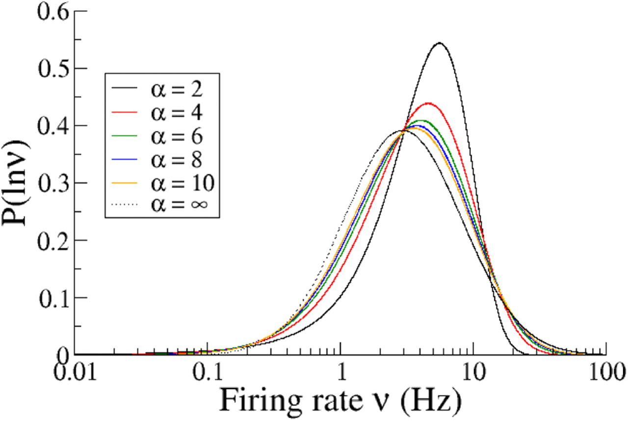
Distribution of the logarithm of the firing rate for power-law transfer functions with different powers. The mean μ̄ and variance Δ2 of the Gaussian input distribution were adjusted to fix the mean at 5 Hz and the variance of the logarithm of the rate at 1.04. As α is increased, the distribution of the logarithm of the rate approaches a Gaussian distribution, indicating that rate distribution more closely approaches a lognormal distribution (indicated for comparison with a dotted line).
Firing rate distribution for a population of integrate-and-fire neurons with Gaussian distributed inputs
We now consider a population of non-interacting identical LIF neurons in which the voltage, Vi, of neuron i satisfies
 with a threshold voltage θ and reset potential Vr. In Equation 38, τm is the membrane time constant, μi is the time averaged input, σ is the amplitude of temporal fluctuations about the mean, and ηi(t) is a Gaussian white-noise term. This type of input would result from the arrival of a large number of uncorrelated synaptic inputs with fast kinetics compared with τm [using the diffusion approximation (Tuckwell, 1988; Amit and Tsodyks 1991)]. In particular, we will study the mean firing rate of neurons described by Equation 38 in the so-called fluctuation-driven regimen, where μi < θ and σ is sufficiently large to drive spiking. This is the case when the neuron is bombarded by sufficiently strong excitatory and inhibitory inputs, which nearly cancel in the mean. Such a dynamical regimen is robustly observed in recurrent networks of excitatory and inhibitory neurons (van Vreeswijk and Sompolinsky, 1996; Renart et al., 2010). We also assume that the time-averaged input μi, which is distributed across the population, is given by μi = μ̄ + Δzi, where μ̄ is the mean input averaged over all neurons, Δ is the SD of the quenched variability in inputs, and the random variables zi are independently drawn from a Gaussian distribution with mean 0 and variance 1. This type of variability arises in networks in which connections between neurons are made with a fixed probability p. Specifically, the mean input attributable to recurrent connections from a population of N neurons would be proportional to pN, whereas the variance in the number of connections, proportional to p(p − 1) N, leads to nearly Gaussian quenched variability in the input currents (for details, see Materials and Methods). In summary, although Equation 38 describes the dynamics of a population of uncoupled neurons, the statistics of the input currents are chosen to reflect what one would observe in a recurrently coupled network. In this way, we can focus solely on the role of the single-cell f–I curve in shaping the firing rate distribution, given a distribution of input currents. In the following section, we consider a fully recurrent network self-consistently.
The mean firing rate νi of neuron i, whose membrane potential dynamics are described by Equation 38, is then given by νi = ϕ(μi, σ), where ϕ satisfies (Siegert, 1951; Amit and Tsodyks, 1991)
 with x+ = (θ − μ)/σ and x− = (Vr − μ)/σ. This function exhibits three qualitatively different regimens. (1) When the inputs are far below threshold (x+ ≫ 1), the firing rate scales as exp(−x+2) with an algebraic prefactor (see Materials and Methods). Therefore, as the input is reduced, the reduction in firing rates is faster than exponential. This is the low firing rate limit of the f–I curve. (2) When the input currents are in some range close to threshold (x+ = ν(1)), the f–I curve can be well described by a power law (Hansel and van Vreeswijk, 2002). (3) Finally, for suprathreshold input currents (x+, x− ≪ 0), the f–I curve becomes linear, before saturating if an absolute refractory period is added to the model.
For typical parameters of the LIF neurons, imposing a mean firing rate at physiological values (e.g., 5 Hz) yields mean inputs that are in the subthreshold range but not very far from threshold. It follows from these observations that the distribution of firing rates in a population of LIF neurons at physiological levels of activity is in general close to the one obtained with a power-law f–I curve.
We now investigate how varying the noise intensity and membrane time constant of the LIF neuron affects its f–I curve and, consequently, the distribution of firing rates.
Varying the noise intensity σ
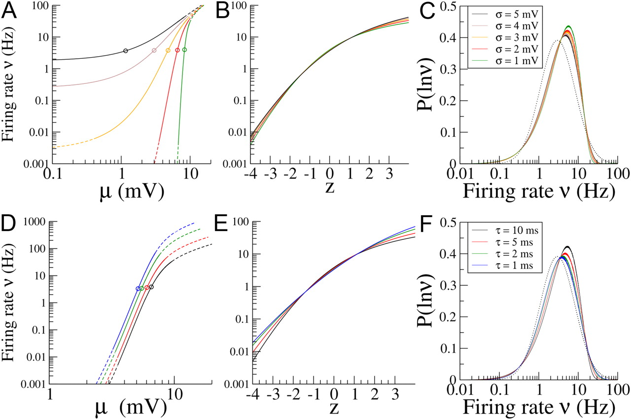
Figure 3A shows the firing rate ν as a function of the input μ on a log–log scale for different values of the noise intensity, σ. On such a log–log plot, a power-law function would show up as a straight line with a slope equal to the exponent of the power law. All of the curves in Figure 3A are concave-up for very low rates (small inputs), whereas for high rates, they all converge to a straight line with slope 1. Between these two limiting behaviors, there is an inflection point around which the curves are approximately linear with a slope >1. Therefore, in this range, the relationship between ν and μ can be well approximated by a power law with an exponent >1. As the noise intensity decreases, the slope of this line increases and the range of firing rates for which the power-law approximation is valid broadens.

Transfer function and firing rate distribution for a population of integrate-and-fire neurons. A, Log–log plot of the firing rate, ν, versus the input, μ, for different values of the noise intensity σ (indicated in C) and with τ = 10 ms. The firing rate approaches a constant value as μ → 0. It increases with σ. On a log–log plot, there is a region for intermediate firing rates in which the f–I curve is approximately a straight line. This corresponds to a power-law f–I relationship with an exponent that increases for decreasing σ. The mean of the input distribution is indicated by an open circle, and the solid portion of each line spans 4 SDs of the input distribution. B, Firing rate as a function of the normalized input z = (μ − μ̄)/Δ on a semi-log plot in which a straight line indicates an exponential dependency. C, Distribution of ln(ν) for different values of σ. The mean and variance of the input was adjusted so that, for all values of σ, the mean firing rate was 5 Hz, and the variance of the logarithm of the firing rates was 1.04. The dotted curve is a lognormal distribution with the same mean and variance. D–F, Same as for A–C but for a fixed value of σ = 2 mV with τ = 10, 5, 2, 1 ms.
To determine the shape of the resulting firing rate distribution for a given f–I curve, we must choose the parameters of the input distribution, μ̄ and Δ. Here, we choose these parameters so that the mean firing rate is 5 Hz, and the variance of the log of the firing rate is 1.04. These values are chosen because they correspond approximately to the experimental data of Hromádka et al. (2008). Clearly, as σ is varied, μ̄ and Δ have to be adjusted to keep the mean and SD of the distribution of log rates constant. In Figure 3A, the range of the f–I curve probed by the distribution of inputs (the region between μ̄ − 4Δ and μ̄ + 4Δ) is indicated by the solid line. It shows that, as σ decreases, the mean of the input distribution has to move closer to threshold, whereas the SD has to decrease, to maintain the first two moments of the distribution of log rates constant. In Figure 3B, we show ν as a function of z = (μ − μ̄)/Δ on a log–linear scale for which an exponential curve would appear as a straight line, for the same values of σ as in Figure 3A. It shows that, for all σ, the logarithm of ν has a sublinear dependence on z. This is attributable to the fact that the f–I curve decays faster than an exponential at low rates, whereas it becomes linear at high rates. The dependence of the curve on σ is rather weak: decreasing σ increases the curvature.
Finally, Figure 3C shows the distribution of the logarithm of the firing rates for a population of integrate-and-fire neurons, for the same values of σ. It shows that, in all cases, the distribution is qualitatively similar to a lognormal but with the differences already described above: an excess of neurons at low rates, together with a dearth of neurons at high rates. It also shows that, although a decrease in σ leads to an increase of the exponent α of the power-law fit close to the inflection point, decreasing σ actually leads to a distribution that becomes less close to a lognormal. This is attributable to the fact that the inflection point decreases with decreasing σ. Therefore, the range of the f–I curve probed by the inputs progressively leaves the region that is well fit by the power law in that limit. If one varies the membrane time constant together with σ, in such a way as to constrain the inflection point to stay close to the mean rate, then the opposite effect is seen: the distribution of rates gets close to a lognormal in the small σ limit (data not shown).
Varying the membrane time constant
For the integrate-and-fire neuron, changes in the membrane time constant are equivalent to a rescaling of the firing rate (see Eq. 19). This is exactly the case only if the refractory period is 0 and is otherwise approximately true for firing rates well below the inverse of the refractory period. This means that, for a given input, decreasing the membrane time constant will lead to an increased firing rate. If we instead choose to fix again the range of firing rates, decreasing the membrane time constant will lead to a decrease in the inputs. This effect is illustrated in Figure 3D. Effectively, this means that the input distribution is shifting toward the low rate tail of the f–I curve as τ decreases. Figure 3E shows log(ν) as a function of z for different values of τ. The curves clearly straighten for decreasing τ. In fact, it can be shown analytically that, in the limit τ → 0, ν becomes an exponential as a function of z, ν(z) = ν0eaz, where ν0 and a are non-zero constants (for details, see Materials and Methods).
Finally, Figure 3F shows firing rate distributions for the same four values of the membrane time constant. The lognormal distribution with this mean and variance is indicated by the dotted line. The distributions clearly become closer to lognormal for decreasing τ, as expected from Figure 3E and the analytical calculation in Materials and Methods.
Varying the mean firing rate
In the previous two sections, we explored the effect of varying the noise intensity and membrane time constant on the shape of firing rate distributions, while keeping the mean of the distribution fixed. Figure 4 shows how the shape of the distribution changes if the mean rate is allowed to vary from 1 to 20 Hz, while holding the variance of the logarithm of the rates fixed. The distribution clearly deviates more strongly from lognormal as the mean rate increases. The reason for this is that neurons firing at higher rates sample the f–I curve outside of the fluctuation-driven regimen. In the suprathreshold regimen, the f–I curve approaches a straight line and the high-rate tail of the distribution therefore shrinks compared with a lognormal.

The distribution of firing rates for a network of uncoupled LIF neurons (Eq. 38) for different values of the population-averaged mean firing rate. Here the mean firing rate averaged over the population increases, while the variance of the log of the rates is held fixed at 1.04. Parameters: τm = 2 ms; μ̄ = 4.73, 5.89, 6.37 mV; Δ2 = 0.187, 0.28, 0.36, 0.5 mV2; σ = 2 mV, lead to v̄ = 1, 5, 10, 20 Hz, respectively.
Firing rate distributions for networks of recurrently connected integrate-and-fire neurons
We now consider a network of randomly connected excitatory and inhibitory integrate-and-fire neurons. For simplicity, we first consider the case in which the single-cell properties, e.g., membrane time constant, of excitatory and inhibitory cells are the same. We also focus on parameter regimens such that the mean synaptic inputs are well below threshold but fluctuations in the membrane potential are large and thus drive spiking activity. As a result, the firing of single cells is irregular.
Figure 5 shows basic features of the activity of a network of NE = 10,000 excitatory and NI = 2500 inhibitory neurons, which are randomly connected with a connection probability p = 0.1. Random connectivity means that the distribution of the number of excitatory and inhibitory synaptic inputs across the network is approximately Gaussian, as shown in the inset of Figure 5A. Consequently, the distribution of time-averaged synaptic inputs is also close to Gaussian, as shown in Figure 5A. Figure 5B shows a raster plot of 30 cells chosen at random; it is clear that the firing is irregular and that firing rates are broadly distributed. The voltage trace of neuron number 1 is shown in the bottom of Figure 5B and clearly exhibits strong temporal fluctuations.

Firing rate distributions in randomly connected networks of LIF neurons in an asynchronous irregular state. A, The distribution of mean inputs across neurons in the LIF network. The solid line was generated numerically from a run of 10 s, and the dashed line is a Gaussian function, the mean and variance of which are given by Equations 15 and 16, respectively. The inset shows the distributions of excitatory (exc) and inhibitory (inh) connections (with means 1000 and 250 subtracted off, respectively), which are also close to Gaussian. B, The top panel shows a raster diagram of the activity of 30 randomly chosen neurons from the simulation. The bottom panel is the membrane voltage of one neuron. Both the spiking and subthreshold activities are irregular. C, The numerically determined firing rate distributions from a simulation lasting 10 s. The mean of the distribution is indicated by the white arrow, and the median is indicated by the black arrow. D, The distribution of the logarithm of the firing rate. Results from the simulation are shown as filled symbols in which the error bars show the SD over 10 runs of 10 s each. The solid line is the best-fit lognormal distribution. Note that there is an excess of neurons firing at low rates and a dearth of neurons firing at high rates in the simulation compared with the lognormal fit. Parameter values: τE = τI = 20 ms; NE = 10,000; NI = 2500; p = 0.1, θ = 20 mV; Vr = 10 mV; JEE = JIE = JextE = JextI = 0.2 mV; JII = J EI = −1.2 mV; CextE = CextI = 1000; νextE = νextI = 5.5 Hz.
Given that the network is operating in the fluctuation-driven regimen in which single-cell transfer functions exhibit an expansive nonlinearity, we expect from the analysis described above that the firing rate distributions will not be Gaussian but rather with a peak near 0 and a long tail. This is indeed the case, as shown in Figure 5C by the histogram of firing rates in the network for a simulation of 10 s. The mean and median of the distribution are given by the white and black arrows, respectively, and are ∼6.4 and 5 Hz, respectively. Figure 5D shows the distribution of the logarithm of the firing rate for all cells in the network. Here the filled squares indicate the mean of 10 simulations, each with a different realization of the network connectivity and each 10 s long, whereas the solid line is the best-fit lognormal distribution. Error bars indicate the SD.
Network of excitatory and inhibitory neurons with different properties
In the analysis we have considered thus far, excitatory and inhibitory neurons have been identical. In fact, one physiological characteristic of inhibitory interneurons is their elevated firing rate compared with that of excitatory neurons (Wilson et al., 1994; Haider et al., 2006, 2010). When recording the activity of large ensembles of cells, some fraction of them may be inhibitory, and the resulting firing rate distribution will therefore be a mix of two different distributions: one for excitatory neurons and one for inhibitory neurons. We explore the consequence of this fact by allowing the external input to the inhibitory cells to differ from that of the excitatory cells. Specifically, we increase the external input to the population of inhibitory cells compared with that of the excitatory population. This leads the inhibitory cells to fire at higher rates. We then calculate the firing rate distribution for the full recurrent network analytically. Details of the analytical treatment of the network dynamics are discussed in Materials and Methods.
Figure 6 shows the effect of increasing the inhibitory rates on the combined output distribution. Four cases are shown in which the mean firing rate of both populations combined is held fixed at 5 Hz (see legend of Figure 6 for mean firing rates of each population). Allowing for inhibitory neurons to fire at higher rates than the excitatory neurons clearly broadens the tail at high rates. However, once the two firing rate distributions for excitatory and inhibitory cells are sufficiently separated, the resulting firing rate distribution for the full network becomes bimodal. The onset of this effect can be seen in the black curve. This suggests that the similarity of the distribution to a lognormal will be best for intermediate cases.

Distribution of firing rates for a network of two populations in which excitatory and inhibitory neurons fire at different mean rates. Shown are three firing rate distributions calculated analytically from Equation 22. The blue one shows the case of identical firing rates in both populations of neurons. The red, black, and orange curves show how the distribution changes as the inhibitory cells fire at increasingly higher rates. The clearest effect is the broadening of the tail at high rates. In all cases, the mean and SD of the log rates have been fixed. The dotted curve is a lognormal distribution with the same mean and SD. Parameters: νextE = 23, 30.35, 32.9, 47.05 Hz; νextI = 23, 32.55, 35.95, 50.68 Hz; ΔC2 = 2000, 620, 50, 0; JEE = JIE = JextE = JextI = 0.0713, 0.0713, 0.0713, 0.048 mV; JII = JEI = −6JEE mV for the blue, red, black, and orange curves, respectively. The remaining parameters are the same: τE = τI = 5 ms; CextE = CextI = 1000.
Comparison of network of LIF neurons with in vivo data
We have shown that the distribution of firing rates in networks of LIF neurons is significantly right skewed in the fluctuation-driven regimen. Furthermore, although the distribution is close to lognormal over a wide range of values of single-cell properties and mean firing rates, there are consistent deviations: there are fewer high-rate neurons and more low-rate neurons than predicted by a lognormal fit. Here we see how well a network of LIF neurons can fit firing rate distributions from in vivo recordings and whether the predicted deviations can be observed. Figure 7A shows the firing rate distribution obtained from a simulation of the integrate-and-fire network with two populations of neurons and an elevated firing rate of inhibitory neurons compared with the excitatory neurons (νE = 3.5 Hz, νI = 11 Hz) (black symbols). The solid line is the analytical curve predicted from Equation 22. The firing rate distribution from simulation is close to the one obtained experimentally during spontaneous activity in the auditory cortex of unanesthetized rats (Hromádka et al., 2008) (red symbols). Figure 7B shows the fit of a network of LIF neurons (solid line; Eq. 22) to the activity of 92 neurons from barrel cortex of awake, head-restrained mice (O'Connor et al., 2010) (symbols). The firing rate of each cell is an average over several epochs of an object localization task. The distributions found from taking rates during any one of the epochs individually is qualitatively similar. The best-fit lognormal is shown for comparison as a dashed line.

Comparison of results from LIF network and experimental data. Distributions of the logarithm of the firing rate. A, Black, From 10 simulations, each with a different realization of network connectivity, of 10 s duration each; error bars indicate 2 SDs. Red, From spontaneously active neurons in auditory cortex; error bars indicate 95% confidence intervals. Solid line, Analytically determined distribution from Equation 22. Parameters for the simulations: τE = 5 ms; τI = 2.5 ms; NE = 8000; NI = 2000; p = 0.125; θ = 10 mV; Vr = 0 mV; JEE = JextE = 0.188935 mV; JIE = JextI = 1.75 JEE mV; JEI = −3.5 JEE mV; JII = −3.5J IE mV; CextE = CextI = 1000; ΔC2 = 2000; νextE = 10.29 Hz; νextI = 9.99 Hz. There is a uniform distribution in synaptic delays from 0.1 to 3.1 ms. B, Black circles, From barrel cortex of awake mice. Solid line, Analytically determined distribution from a network of uncoupled LIF neurons (Eq. 22) with μ = 4.85 mV, σ = 2.2 mV and Δ =
 mV. Dashed line, Best fit to a lognormal distribution.
In Figure 7B, we see that the O'Connor et al. data exhibit the deviations from the lognormal that are predicted by the theory: an excess of neurons at low rates compared with a lognormal, as well as a dearth of high-rate neurons. In fact, the figure shows that the distribution of an LIF network with appropriately chosen parameters fits the data much better than a lognormal.
Firing rate distributions in large networks of conductance-based neurons
We have shown how the distribution of firing rates in a randomly connected network of LIF neurons is generically right skewed and can in some cases be well approximated by a lognormal distribution. We have chosen to focus on LIF neurons because they are one of the few spiking neuron models to allow for analytical treatment, and their f–I curves have been shown to fit reasonably well f–I curves of cortical neurons in the presence of noise (Rauch et al., 2003). Nonetheless, to show that our results are general, we conducted simulations of networks of randomly connected conductance-based neurons, the dynamics of which follow a Hodgkin–Huxley formalism. The interactions between the neurons were also conductance based (in contrast with the LIF network considered above in which they were current based).
We first consider the case with no heterogeneities in the synaptic conductances, i.e., σg = 0 in Equation 37. Figure 8, A and B, shows traces of the membrane voltage from three excitatory neurons (A) and three inhibitory neurons (B) in the network. Membrane voltage fluctuations are large while the mean voltage is subthreshold. This leads to highly irregular spiking. This irregularity is quantified in Figure 8C in which the distribution of the coefficient of variation (CV) of the interspike interval distribution is shown for excitatory and inhibitory neurons. The two histograms are sharply peaked at approximately CV ≈ 1.1. Similar to what we found in the LIF model analyzed above, the distribution of the firing rates of the neurons in this conductance-based network is right skewed. The average (over E and I populations) firing rate is 4.9 Hz, whereas the median firing rate is more than a factor of 2 lower, with a value of 2.2 Hz. Figure 8D displays this distribution on a semi-log plot. Fitting the data to a Gaussian (solid line) indicates that they can be well approximated by a lognormal, although small deviations are observed at very low firing rates (an excess of neurons <0.2 Hz) and at high firing rates (a lack of neurons >60 Hz).

Firing rate distributions in a network of conductance-based neurons in the fluctuation-driven regimen. Parameters are given in Material and Methods. A, Sample traces from three excitatory neurons. B, Sample traces from three inhibitory neurons. C, The distributions of CVs of excitatory neurons (black line) and inhibitory neurons (red line). D, The firing rate distributions, for several values of σg, indicated on the figure. Symbols are from simulations, and lines are best-fit lognormals. Parameters are given in Material and Methods. In A–C, σg = 0.
Recent experimental findings, obtained from paired intracellular recording in cortical slices, indicate that the distribution of synaptic strength in cortex is skewed and close to a lognormal distribution (Song et al., 2005). Therefore, we also considered networks in which the maximum synaptic conductances are lognormally distributed (see Material and Methods) with a mean of the log conductance such that the average conductance remains constant as the SD of the log conductance, σg, is varied. The network operates in the fluctuation driven regimen, with neurons firing highly irregularly, for all the values of σg we examined (up to σg = 0.8). In all these cases, the firing rate distributions are right skewed as for σg = 0. Although for given values of the external inputs the mean and median changes with σg, the log-rate distribution is well fitted with a Gaussian. The results are shown in Figure 8D. Somewhat counterintuitively, we found that the width of the firing rate distribution decreases when σg increases. This effect can be understood by analyzing the impact of synaptic heterogeneities on the distribution of rates in the simpler network of LIF neurons (see Materials and Methods).
Discussion
We have studied firing rate distributions in sparsely, randomly connected networks operating in the fluctuation-driven regimen, i.e., when spiking occurs because of positive fluctuations in the synaptic noisy input. In this regimen, the in vivo f–I curve exhibits an expansive nonlinearity in the physiological range of firing rates as a result of this noise. This nonlinearity transforms the relatively narrow, Gaussian distribution of time-averaged inputs to the neurons (which is attributable to the variability in the number and in the efficacies of synaptic contacts) into outputs with a right-skewed, long-tailed distribution. This mechanism is very robust, as we have shown by using both analytical methods and numerical simulations: broad distributions of firing rates are found in rate models with power-law transduction functions, in networks of current-based integrate-and-fire neurons, as well as in networks of conductance-based Hodgkin–Huxley-type neurons. In no case do the relevant parameters require fine-tuning. We stress that the proposed account for the origin of spatial inhomogeneity in the patterns of network activity also naturally explains the temporal irregularity in spiking that is observed during the same recordings.
Some authors observe large infrequent synchronized barrages of synaptic inputs (“bumps”) in rodent auditory cortex in vivo (DeWeese and Zador, 2006). This is consistent with a “shot-noise” model of synaptic inputs with very large amplitudes. It can be shown that f–I curves of LIF neurons in the presence of such inputs also exhibit an expansive nonlinearity (Richardson and Swarbrick, 2010). Therefore, we expect our results to apply qualitatively also in this situation.
One counterintuitive result of our analysis is that increasing the width of the distribution of synaptic weights decreases the width of the firing rate distribution. An analytical investigation of the low τ limit in the network of LIF neurons allows us to understand the origin of this phenomenon: although a broader distribution of synaptic weights leads to an increase in the width of the input distribution, it also changes the shape of the f–I curve through the variance of the temporal fluctuations received by neurons. The f–I curve becomes less steep and, as a result, the distribution of rates becomes narrower.
Our analysis indicates that, for homogeneous neuronal populations, a lognormal distribution of firing rates is, in general, not to be expected. The rate distribution becomes lognormal in the limit in which the exponent of the power-law diverges and in the limit in which the membrane time constant goes to 0. Clearly, both of these limits are physiologically implausible. Moderately large exponents (α = 3–5) and short time constants (τ = 5–10 ms), both well within reported physiological ranges, lead however to firing rate distributions that are very close to lognormal. Moreover, as we have illustrated in a simple case (e.g., excitatory and inhibitory populations with different activity levels), heterogeneities in neuronal properties can lead to firing rate distributions that are closer to lognormal than those seen in the case of the homogeneous populations. Besides differences in firing rate for excitatory and inhibitory cells, other heterogeneities (not considered in the present study) are well documented: average activity levels and rate distributions change depending on the cortical layer (Sakata and Harris, 2009; O'Connor et al., 2010) and on the cell types (de Kock and Sakmann, 2009). Moreover, some cells exhibit so low a firing rate that they could easily go unnoticed, unless explicitly looked for. A case in point is the study by O'Connor et al. (2010), in which ∼10% of the neuronal sample is made up of “silent neurons,” i.e., with an upper bound firing rate <0.0083 Hz. Indeed, in our fit to the data from the study by O'Connor et al. (2010), we do not include the silent cells, which would here add a delta function component at zero rate.
Our conclusions are in stark contrast to the conclusions of a recent theoretical study (Koulakov et al., 2009). In that study, the authors analyzed a network rate model with linear f–I curves. In such a network, a Gaussian distribution of inputs leads to a Gaussian distribution of rates. At the same time, unless strong correlations among afferent inputs are present, the distribution of inputs in a large network will be Gaussian because of the central limit theorem. Therefore, because of the linearity of their model, the authors assume the presence of strong correlations in synaptic input such that the distribution of inputs is lognormal. This then leads to a lognormal distribution of firing rates. We note here that lognormal input distributions lead to lognormal rate distributions only in the case of a linear f–I curve. Although our study does not rule out the presence of input correlations, it shows that the well documented nonlinearity of the f–I curve in in vivo conditions is mostly sufficient to account for lognormal-like firing rate distributions.
Although we have been able to account for the firing rate distribution in the fluctuation-driven regimen in rather general terms, one important simplification we have made is to assume random connectivity in the standard sense: connections between neurons are made with a fixed probability. In fact, there is growing experimental evidence that the connectivity in cortical networks deviates from a standard randomly connected network, i.e., one in which connections are made independently with a fixed probability (Song et al., 2005; Yoshimura et al., 2005; Wang et al., 2006). In particular, it may be that some degree of input correlation is present in cortical networks and the input distribution therefore deviates from Gaussian. However, the results presented here should not be qualitatively affected by weak-to-moderate correlations in the synaptic inputs to neurons.
Footnotes
-
A.R. was supported by the Gatsby Foundation, the Kavli Foundation, and the Sloan-Swartz Foundation. A.R. was also a recipient of a fellowship from IDIBAPS Post-Doctoral Programme that was cofunded by the European Community under the BIOTRACK project (Contract PCOFUND-GA-2008-229673) and was additionally funded by the Spanish Ministry of Science and Innovation (Grant BFU2009-09537) and the European Regional Development Fund. The research of D.H., G.M., and C.v.V. was supported in part by Agence Nationale de la Recherche under Grant 09-SYSC-002. D.H. and C.v.V. were also supported in part by National Science Foundation Grant PHY05-51164 and thank the Kavli Institute of Theoretical Physics at University of California Santa Barbara and the program “Emerging Techniques in Neuroscience” for their warm hospitality while writing this manuscript. We thank Daniel O'Connor and Karel Svoboda for the use of their data.
-
The authors declare no competing financial interests.
- Correspondence should be addressed to Alex Roxin, Insitut d'Investigacions Biomèdiques August Pi i Sunyer, Carrer del Rosselló 149, Barcelona 08036, Spain. aroxin{at}clinic.ub.es


