

Abstract
Although the neural processing of chromatic and spatial features is intertwined, it is unknown how consistent this spatio-chromatic coding is across different brains. In this fMRI study we predicted the color a person was seeing using a classifier that has never been trained on chromatic responses from that same brain, solely by taking into account: (1) chromatic responses in other individuals’ brains and (2) commonalities between spatial coding in brains used for training and the test brain. Fitting shared response models to fMRI responses elicited by spatially defined and achromatic retinotopic mapping stimuli, we transformed subject-specific color responses to a common functional space. In this space we successfully decoded color across observers based on activity patterns in V1-V3, hV4 and LO1. Examining classification weights, we found that systematic large-scale retinotopic biases for the different colors may explain at least partially the observed agreement of neural color coding between brains.
Introduction
It is an age-old question whetherthe subjective experience one person has of a given color matches that of another person. While it is difficult to answer this directly, it is possible to answer a related question: are there similarities in neural representations of colors that are shared across brains? In the present study we used a method called shared response modeling to address this question. By projecting each participant’s neural representations into a shared neural space that was independent of color, and defined purely by achromatic spatial information, we implicitly also addressed the question to which extent color and spatial information are coupled across brains.
In humans, color vision has traditionally been thought to be mediated by functionally segregated neural mechanisms already at earliest stages of visual processing (De Valois and Jacobs, 1968; Zeki, 1973; Derrington et al., 1984; Schiller et al., 1990; Field and Chichilnisky, 2007), consistent with the “opponent process-theory of color vision”.
Specifically, early electrophysiological work suggested that color signals were processed independently from spatial signals in the LGN and visual cortex-with spatial information being encoded in the cytochrome-oxidase (CO) poor regions and color being encoded along the CO rich “blob” and “thin stripe” regions in areas V1 and V2, respectively (Livingstone and Hubel, 1984, 1988; Ts’o and Gilbert, 1988; Schiller et al., 1990; Lu and Roe, 2008; Denison et al., 2014; Nasr et al., 2016), and in localized clusters called “globs” in V4 (Conway et al., 2007; Conway and Tsao, 2009). Relatedly, functional dissociations between visual areas for chromatic and spatial processing had been reported at a larger spatial scale: lesions in the medial fusiform gyrus can lead to color blindness while sparing object and motion vision, and correspondingly, neural color responses were found in area V4 and its satellites (Zeki, 1978, 1980b, a; Lueck et al., 1989; Zeki et al., 1991; Beauchamp et al., 1999; Bartels and Zeki, 2000).
However, it has also been argued thatthe computations underlying color constancy necessitate the integration of chromatic and spatial signals (Land and McCann, 1971; Land, 1986; Rüttiger et al., 1999; Brainard, 2009; Moutoussis, 2015). In accord with this, numerous studies found evidence for joint neural coding of chromatic and spatial information (Leventhal et al., 1995; Kiper et al., 1997; Johnson et al., 2001, 2008; Friedman et al., 2003; Sincich and Horton, 2005; Garg et al., 2019). A relevant mechanism in this respect may consist in the adaptation of neural responses in both primary (Wachtler et al., 2003) and extrastriate visual areas (Kusunoki et al., 2006) of the monkey brain in response to chromatic modulations of spatial context. In the human brain, color surface represen-tations that are robust against illumination changes serve a similar purpose for color constancy computations as well (Bannert and Bartels, 2017). Several behavioral phenomena demonstrate the interdependence between spatial and chromatic processing (reviewed by Moutoussis, 2015): color experience thus depends on the interpretation of an ambiguous 3D figure as either convex or concave (Bloj et al., 1999; Kingdom, 2003), on the orientation of an afterimage-inducing grating (McCollough, 1965; Vul and MacLeod, 2006). Border (Ware and Cowan, 1982; Pinna et al., 2001; Monnier and Shevell, 2003) and filling-in effects (Krauskopf, 1963; Hsieh and Tse, 2006, 2009) like-wise exemplify well-known spatiochromatic interactions.
Accordingly, human neuroimaging found that orientation adaptation effects in the fMRI signal were chromatically specific in a way that mirrors perception (Engel and Furmanski, 2001; Engel, 2005). Pattern classification analyses of BOLD responses similarly showed that the fine-grained spatial orientation responses were specific to chromatic contrast (Sumner et al., 2008). Using the same approach, it is possible to decode from fMRI responses which of two possible pairings of color and motion direction was presented to an observer (Seymour et al., 2009, 2010). This form of conjunctive encoding of the two visual features may in fact be one of the brain’s mechanisms to solve the binding problem (Di Lollo, 2012). Interestingly, conjunctive spatio-chromatic coding is found primarily in the deep and superficial feedback layers of monkey V2 (Shipp et al., 2009), consistent with the putative role of attention for feature binding (Treisman, 1988).
Our research aim was to examine to what extent spatial and chromatic stimulus features were simultaneously encoded in brain activity. Specifically, we were interested to learn how consistent such co-representation would be across different brains.
Here, we addressed these questions by aligning subject-specific fMRI response spaces to each other using shared response modeling. In contrast to previous similar cross-subject alignment approaches (Haxby et al., 2011; Guntupalli et al., 2016), we used brain responses evoked by the spatially changing position of slowly moving achromatic checkerboard stimuli used for retinotopic mapping. Individual brain activity was hence sampled in response to a highly restricted subset of stimulus inputs comprised of purely spatial variability in the absence of chromatic stimulation. This allowed us to ensure that the stimulus properties that were used for estimation of shared neural responses were based solely on spatial information. If conjunctive neural representations of space and color are indeed shared across observers, it should be possible to predict from an observer’s pattern of brain activity what color the person was seeing using a classification model that was trained solely on other observers’ brain responses to color, i.e. to classify color across the brains of different participants. Our findings showed this to betrue, and further suggest that the observed between-subject decoding is mediated by common spatio-chromatic representations that are at least in part embodied by large-scale retinotopic biases shared between brains.
Results
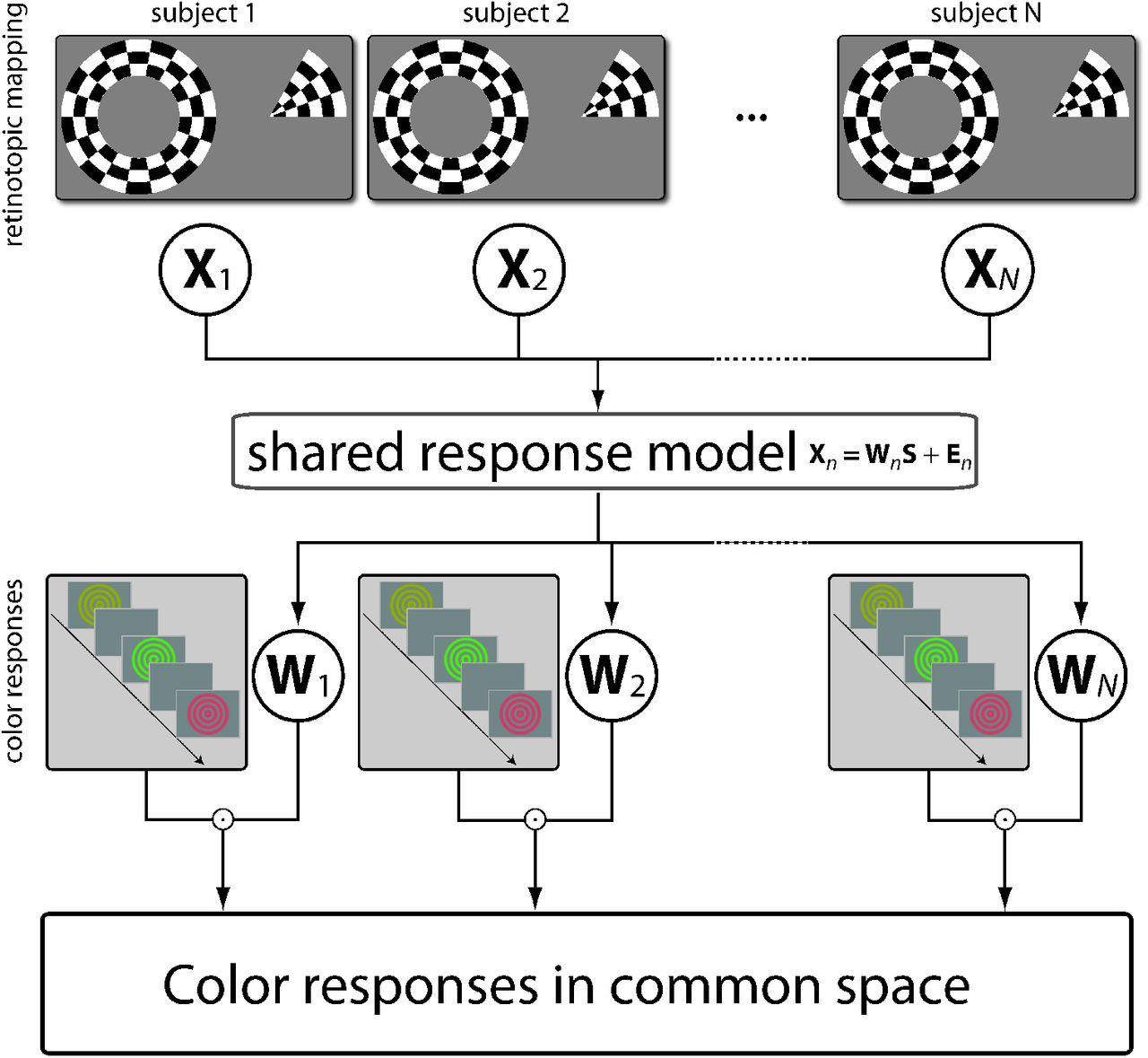
The goal of the experiment was to examine whether representations of chromatic signals were shared across human brains and whether this occurs in a spatial neural code. Specifically, our hypothesis was that chromatic signals may share aspects of spatial, achromatic representations that are conserved across different individuals. For this reason, we used brain responses to achromatic, spatial stimuli to construct a neural space that was shared between observers Figure 1. We then tested whether this neural space generalized to decode color responses in specific, individual brains from color responses in other observers’ brains – in other words – to predict color across brains.

Retinotopic mapping data (top) were recorded while participants watched a rotating wedge or an expanding/contracting ring stimulus. Datasets from every participant’s ROI were resampled to the same temporal resolution and entered into a shared response model (Chen et al., 2015; Anderson et al., 2016). SRM estimates a transformation matrix Wn for every participant mapping voxel response spaces from individual ROIs into a 50-dimensional common space (see Materials and Methods). Note that only retinotopic mapping data were used to estimate transformation matrices. Color responses (bottom) were measured with fMRI from participants performing a luminance change detection task on red, green, and yellow ring stimuli presented at two luminance levels. Stimuli were shown for 8.5 s with ITI = 1.5 s (see Materials and Methods). Using the Wn matrices, these fMRI color responses in every ROI and participant, which were recorded independently from the retinotopic mapping data, were mapped from individual response spaces into the common space.
Within-subject classification of color and luminance (WSC)
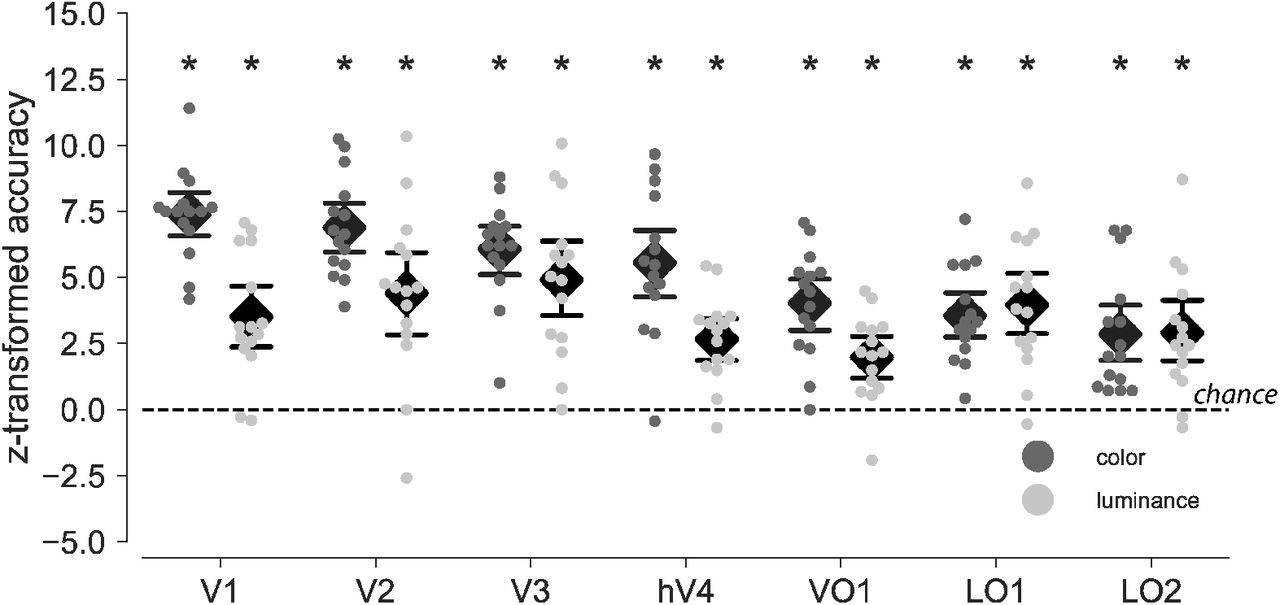
Decoding color across different brains requires that color can be decoded within one and the same individual brain. For this reason we first performed pattern classification analyses on fMRI activity from ROIs at the level of individual subjects. The same logic applied to luminance decoding. Figure 2 shows classification accuracies z-transformed (n = 216) individually and then averaged across participants (n = 15). Color as well as luminance could be decoded significantly better than chance in all ROIs under investigation (permutation tests, each p < .01, FWE-corrected for seven ROIs). For color (chance level: 33 %), the following classification accuracies applied for each ROI, averaged across participants. V1: 57 % (z = 7.38, 95 % CI [6.51, 8.25]), V2: 55.4 % (z = 6.89, 95 % CI [5.94, 7.84]), V3: 52.84 % (z = 6.08, 95 % CI [5.13, 7.03]), hV4: 51.2 % (z = 5.56, 95 % CI [4.21, 6.91]), VO1: 46.3 % (z = 4.03, 95 % CI [3.01, 5.05]), LO1: 44.8 % (z = 3.56, 95 % CI [2.66, 4.46]), LO2: 42.5 % (z = 2.86, 95 % CI [1.72,4]). For luminance (chance level: 50 %), classification accuracies were as follows. V1: 61.9 % (z = 3.51,95 % CI [2.32, 4.7]), V2: 65 % (z = 4.41,95 % CI [2.81, 6.01]), V3: 66.7 % (z = 4.92, 95 % CI [3.45, 6.38]), hV4: 59.1 % (z = 2.67, 95 % CI [1.84, 3.5]), VO1: 56.7 % (z = 1.98, 95 % CI [1.16, 2.8]), LO1: 63.5% (z = 3.96, 95% CI [2.71,5.22]), LO2: 59.9 % (z = 2.9, 95 % CI [1.69, 4.11]). Individual response patterns in every ROI thus were reliable enough across fMRI runs to linearly predict color and luminance condition.

For every ROI and participant, cross-validated (leave-one-run-out) classification accuracies were obtained for the prediction of color (dark dots) and luminance (light dots). Accuracies are tranformed to z-values using the normal approximation to the binomial distribution (n = 216) so that both classifications share the same y-axis and accuracies expected by chance is 0 in both cases. Black diamonds indicate mean accuracy averaged across participiants and error bars represent the parametric 95 % CI. Asterisks mark accuracies with p values below .01 (permutation tests, 2000 iterations, FWE corrected across 7 ROIs). As shown, classification accuracies were significantly larger than chance for both color and luminance classification.
Between-subject classification of color and luminance (BSC)
Next, we quantified how consistent chromatic neural processing was across individual brains within a neural space that was shared across subjects and defined by responses elicited by a solely achromatic and spatially defined retinotopic mapping stimulus. Individual color responses were mapped from independent measurements to that shared response space, and the classifiers were trained to predict the color (or luminance) of the stimulus a person was seeing. In contrast to WSC, fitted classification models were cross-validated across participants instead of runs. As can be seen in Figure 3, accuracies for luminance and color classification across different brains significantly exceeded chance in areas V1-V3. Additionally, color could be decoded across participants significantly better than chance in areas hV4 and LO1 (permutation tests, p < .01, FWE-corrected for seven ROIs). For each ROI, significant BSC accuracies for color were as follows. V1: 41.3 % (z = 9.62, 95 % CI [7.2, 11.96]), V2: 37.5 % (z = 5.03, 95 % CI [2.64, 7.41]), V3: 40.9 % (z = 9.09, 95 % CI [6.73,11.57]), hV4: 37.7 % (z = 5.33, 95 % CI [2.93, 7.78]), LO1: 38.9 % (z = 6.71, 95 % CI [4.32, 9.06]). For luminance, significant classification accuracies were as follows. V1: 57.1 % (z = 8.12, 95 % CI [5.67, 10.8]), V2: 55.4 % (z = 6.15, 95 % CI [3.73, 8.65]), V3: 53.8 % (z = 4.36, 95 % CI [1.9, 6.86]). This suggests that measurements of how purely spatially defined stimulation activates the brains of different individuals is sufficient to predict colors and luminance from brain activity in any one of them using a classifier trained on data from the remaining participants.

Individual responses were transformed to the common space. Transformation matrices were estimated using the shared response model fit to an independent sets of retinotopic mapping data. Classification accuracies are cross-validated by leaving out the participant during classifier training whose data were used for testing (leave-one-subject-out). The normal approximation to the binomial distribution was used to convert accuracies to z-values (n = 3240). Note that prediction accuracies are represented as bars rather than individual dots (see Figure 2) because the prediction accuracies for individual participants are no longer independent. Error bars denote the 2.5th and the 97.5th percentile of the permuted null distributions. Asterisks denote accuracies significantly exceeding chance at p < .01 (permutation tests, 2000 iterations, FWE corrected across 7 ROIs). Both color and luminance could be predicted across subjects from areas V1-V3. Additionally, color could be predicted from hV4 and LO1.
Retinotopic analysis of classification weights
Since we observed significant BSC across brains after estimating shared responses from the retinotopic mapping experiments, we were interested in a closer examination of any large-scale retinotopic biases mediating these effects. In short, we wanted to learn how the classification rules (i.e., weights), which were learned by LDA during BSC classification and which would allow significant decoding about the color that was presented, were related to retinotopic locations within a given ROI. To that end, a linear classifier was fit to all participants’ data after projection into the shared common space. We mapped back classification weights into individual participants’voxel spaces and combined them with retinotopic coordinates. We then used nearest neighbor classifiers to predict from retinotopic coordinates in each voxel which class it preferred while cross-validating across participants. We thus obtained a visual field map of class preference for every ROI (see Materials and Methods and Figure 4 for details).

(A) For every RO I, an LDA classifier was trained on the common space responses from all participants. The weights were transformed back into individual response spaces such that every voxel was assigned with one weight per class. A nearest neighbor classifier was trained for every voxel to predict based on its Cartesian retinotopic coordinates which class had the highest weight. Every voxel in every ROI and participant thus obtained a predicted class label that was cross-validated across participants. These class predictions were used to quantify the relative preference for a given class as a function of retinotopic location. For each class separately, the retinotopic coordinates of all voxels preferring that class were entered into kernel density estimation to approximate this function. A second function was approximated using all voxels combined, which was subtracted from each of the class-specific functions to normalize them. (B) Results for green, red, and yel low classes (from left to right) in area V1. Colored areas represent visual field locations with a relative overrepresentation of voxels preferring that class while gray areas denote regions with a relative underrepresentation. 0° marks the right horizontal visual meridian.
Predicting color preference from retinotopic coordinates was significantly better than chance (33 %) in all ROIs except LO2, with the following accuracies. V1: 35.8 % (95 % CI [35.1, 36.5]), V2: 37.7 % (95 % CI [37, 38.4]), V3: 37.9 % (95 % CI [37.1, 38.7]), hV3: 37.7 % (95 % CI [36.7, 38.8]), VO1: 36.7 % (95 % CI [35.5, 38]), LO1: 35.9 % (95 % CI [34.6, 37.2]) (all p < .01), LO2: 34.2 % (95 % CI [33.1, 35.4]) (p < .05, permutation tests with 1000 iterations, Holm-Šidák corrected for seven ROIs). Figure 5 shows the class preference maps for color classification. Descriptively, the results showed a systematic relationship between visual field location and color preference. In V3 for instance voxels representing parafoveal locations showed a preference for yellow. At intermediate eccentricities along the horizontal meridian the analysis revealed a preference for green. More peripherally, our analysis showed a preference for red in the upper and lower visual fields.

Same conventions as in Figure 4(B). On the left, p values indicate that nearest neighbor classification of class preference was significantly above chance in all regions tested (Holm-Šidák corrected for seven ROIs). Classes showed distinctive topographies that differed particularly along visual meridians.
Interestingly, the maps show some variability across ROIs. For example, whereas in V3 the yellow stimulus was preferred at parafoveal locations, this was not the case in V1, where preference for yellow was more pronounced at more peripheral locations.
In the case of luminance classification, predicting stimulus preference from retinotopic coordinates was also significantly larger than chance (50 %) in many ROIs, with the following accuracies. V1: 54.2 % (95 % CI [53.5, 55]), V2: 54.8 % (95 % CI [53.9, 55.5]), V3: 54.4 % (95 % CI [53.6, 55.2]), hV4: 52.7 % (95 % CI [51.5, 54]), LO1: 51.7 % (95 % CI [50.4, 53.1]) (p < .05, all Holm-Šidák corrected for seven ROIs). Classification accuracies did not, however, significantly exceed chance in VO1 (50.1 %, 95 % CI [48.7, 51.4], p = .4605, uncorrected) and LO2 (49.8 %, 95 % CI [48.5, 51], p = .6763, un-corrected, permutation tests with 103 iterations.). Descriptively, preference maps again differed across brain regions (Figure 6): While in V1 and V2 the preference for stimulation at high luminance increased with increasing eccentricity for instance, this preference first dropped at intermediate eccentricities relative to central visual field representations before it increased again in the visual periphery.
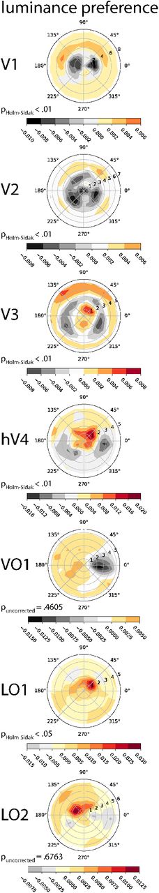
Same conventions as in Figure 4(B). except that since classification was binary, hot areas mark regions in the visual field where high luminance was preferred and gray areas mark regions where low luminance was preferred. On the left, p values indicate that nearest neighbor classification of class preference was significantly above chance in all regions tested except VO1 and LO2 (Holm-Šidák corrected for seven ROIs). In early areas V1-V3 for instance, luminance preference changed as a function of eccentricity. Note that although VO1 showed a difference between left and right visual field descriptively, preference classification in this area (and in LO2 likewise) was not significant.
In sum, these results indicate a systematic relationship between a voxel’s retinotopic spatial preference and its response pattern to color and luminance that could at least partially mediate between-subject classification.
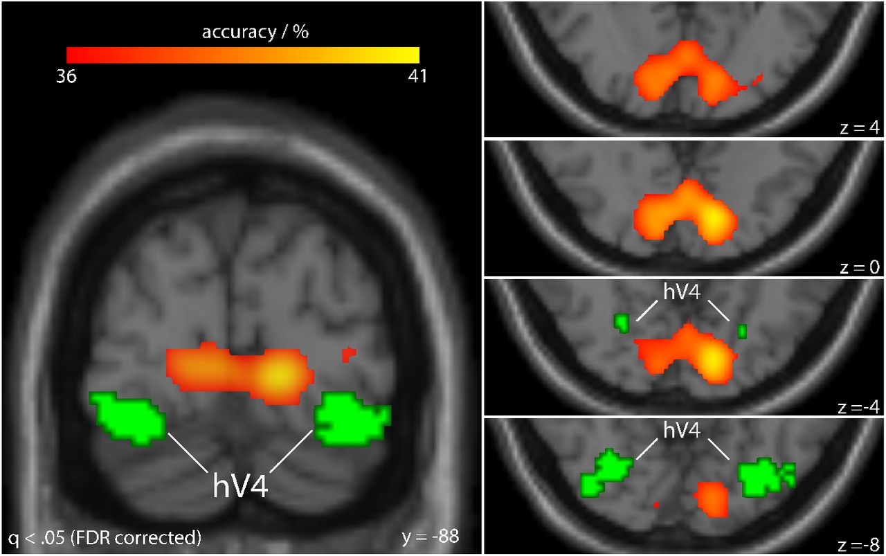
Whole-brain searchlight analysis of shared responses
The ROI results showed that color could be classified significantly better than chance across different brains if classification was performed in a shared response space estimated from responses to only achromatic and spatial stimulation. Yet although the data for these BSC analyses came from different brains, they were recorded in ROIs that corresponded to the same retinotopic field maps. Despite the interindividual variability in the locations of visual areas, they tend to overlap anatomically in standard MNI space.
We therefore tested how well common shared responses could already be estimated from only anatomically aligned activity patterns for subsequent BSC. Individual datasets were warped to MNI space separately and SRM was fit to only local patterns of retinotopic mapping responses in a searchlight analysis to estimate common space representations for every brain location. After transforming individual color responses to this common space, BSC could be carried out on those local patterns. This approach had the additional advantage that BSC could be applied to the whole brain.
Applying a false discovery rate of q < .05, we found that classification accuracies in a region within the early visual cortex was significantly larger than chance (one-tailed binomial test based on 3240 Bernoulli trials). Figure 7 shows the location of this region relative to the hV4 group ROI. This ROI comprised all the voxels that were identified as being part of individual hV4 ROIs in at least 25 % of the participants. As can be seen, the voxels where classification was significantly better than chance were located near the calcarine sulcus but did not overlap with the hV4 group ROI.
SRMs were fit to patterns within local spheres (3 voxel radius) of brain responses to the retinotopic mapping stimulus. After transforming every participant’s dataset into the common space, classifiers were used to predict the color of the viewed image using only the information in the local activity pattern (BSC). Cross-validation was performed by leaving out data from a different participant for testing on every iteration. Classification accuracies are shown in warm colors on a standard MNI template for brain regions that survived the whole-brain significance threshold of a binomial test (q < .05, FDR corrected). Green marks all voxels falling within area hV4 in at least 25 % of the participants. The regions where BSC of color yielded accuracies significantly above chance, namely near the calcarine sulcus, were distinctly different from the location of hV4. This indicates that anatomical alignment was not sufficient beyond earliest visual areas for BSC (e.g. in hV4).
In sum, the searchlight analysis suggests that while anatomical alignment of voxels was sufficiently high for BSC of color in early visual cortex this alignment was too coarse in more anterior regions.
Discussion
Here we tested whether chromatic processing is sufficiently similar between human brains to allow decoding of color across different observers. In particular, we examined this question in a neural space based on purely spatial and achromatic stimulation. We hence exploited dependencies between spatial processing with chromatic processing, for which there is growing evidence Johnson et al., 2001, 2008; Friedman et al., 2003; Engel, 2005; Seymour et al., 2009; Garg et al., 2019). Here we followed up on this research by testing if integrated spatiochromatic processing is sufficiently similar between human brains to allow decoding of color across different observers based on their shared responses to only spatial and achromatic stimulation.
We found that, after taking into account how different brains respond to the same, purely spatially defined retinotopic mapping stimulus, there was a strong agreement across participants between the fMRI activity patterns elicited by stimuli of different luminance and color. Otherwise it would not be possible to linearly classify what color a person was seeing based on their brain activity using only the shared responses to the retinotopic mapping stimulus, i.e. without training the classifier on actual color responses from that particular brain. This is consistent with previous reports of integrated spatiochromatic processing. Yet crucially, it follows from this observation that the relationship between the specific way that the brain represents spatial and chromatic visual features is to some degree preserved across individuals.
Upon further exploration of the nature of this relationship we discovered systematic retinotopic response biases to color as well as luminance. Specifically, we observed that visual field coordinates in a voxel predicted for which color or luminance level that voxel was most predictive. Mapping voxel preferences across the visual field revealed response biases that correlated with eccentricity in a continuous (e.g. V1 in Figure 5) or inverted-U shaped manner (e.g. V3 in Figure 6). Some retinotopic biases aligned with the vertical (e.g. V2 in Figure 5) or horizontal meridian (e.g. VO1 in Figure 5).
Response biases had been reported initially for stimulus orientation (Freeman et al., 2011, 2013; Sasaki et al., 2006) and motion direction (Beckett et al., 2012) as well as ocular dominance (Larsson et al., 2017). As for color, it has been suggested that chromatic response biases in V1 result from neural adaptation to the statistics of natural daylight chromaticities (Lafer-Sousa etal., 2012). In mice, differences in the behavioral significance of stimuli in the upper visual field (above the horizon) versus the lower visual field (below the horizon) may similarly explain differential opsin distributions (Baden et al., 2013; Rhim et al., 2017), which in turn have been related to differences in chromatic discriminatory ability between upper and lower visual fields (Denman et al., 2018).
Focusing, in contrast, on the human color vision, the following paragraphs will discuss studies reporting retinal, behavioral, and cortical chromatic biases in relation to the present findings.
Retinal spatio-chromatic biases
With respect to color, the retinotopic response biases may be related to the distribution of cones in the retina. The fact that cone density decreases with eccentricity (Curcio et al., 1990), that S cones are not found in the fovea (Roorda and Williams, 1999), or that a fourth (melanopsin) photopigment may contribute to peripheral color vision (Horiguchi et al., 2012) could thus be related to differences between preferences at high versus low eccentricities, as we have found for yellow stimuli in V1 for instance. However, the distributions of Land M cones (in contrast to S cones) show large variability across individuals (Brainard, 2015) so that commonalities at the receptor level likely cannot fully explain the observed effects.
Cortical spatio-chromatic biases
With regard to postreceptoral processing, V1 shows a decreasing responsiveness to modulations in the red/green direction in color space, which was not found for the blue/yellow direction (Vanni et al., 2006; Mullen et al., 2007). Although there was no blue in our stimulus set, this is in agreement with our observation of a more pronounced preference for yellow stimuli relative to red and green at high eccentricities in V1 (Figure 5). Interestingly, fMRI activity in one of the studies was strongest close to the horizontal meridian (Vanni et al., 2006), which may be related to the approximate symmetry of the retinotopic pattern of stimulus preference around the vertical axis present in our findings. Note, however, that these previous experiments studied only overall BOLD signal strength in area V1 whereas we used pattern classification analysis in V1 and extrastriate visual areas.
Both in V1 and beyond, examining fMRI contrast sensitivities for gratings (albeit achromatic ones) flashed at various temporal stimulation, an interaction was found between eccentricity and flicker frequency with hV4 responses in contrast to earlier regions correlatingwith behavioral measurements (Himmelberg and Wade, 2019). A comparison between chromatic and achromatic gratings found significant differences between spatial frequency sensitivities of areas V1-V4 at eccentricities of 8-10° but not below 2° of visual angle between the S-cone isolating on the one hand and L-M as well as achromatic gratings on the other (Welbourne et al., 2018).
Behavioral spatio-chromatic biases
Behaviorally, the contrast sensitivities for the chromatic red-green cone mechanism peaks at the fovea and is stronger than for achromatic and blue-yellow mechanisms, yet it also shows the strongest decrease as a function of eccentricity such that it falls below the blue-yellow and achromatic sensitivities at large eccentricities (Mullen, 1991; Mullen and Kingdom, 2002; Hansen et al., 2009).
Spatio-chromatic biases across polar angles
With respect to the dependence upon polar angle, performance effects for the perception of various visual features like contrast, spatial frequency or orientation especially along the horizontal and vertical meridians are well known (Karim and Kojima, 2010; Jóhannesson et al., 2018). Compared to eccentricity dependence, the findings are mixed with some reporting an advantage of the lower visual field for color discrimination relative to the upper visual hemifield (Levine and McAnany, 2005) while others found no differences in any of the hemifield comparisons (Danilova and Mollon, 2009). At the retinal level, cone densities change depending on polar angle in that they are higher along the horizontal than the vertical meridians (Curcio et al., 1990; Song et al., 2011). Simulation has shown, however, that cone density differences as a function of polar angle are too small to account for differences in visual performance at least as far as orientation discrimination is concerned and that postreceptoral, possibly cortical, contributions are therefore likely (Kupers et al., 2019). To what extent these findings generalize to differences in cone ratios and chromatic processing remains an open question.
Regarding cortical effects, human fMRI was able to link the advantage of the lower visual field in an orientation discrimination task to stronger and more extensive activation at the corresponding retinal locations in V1/V2 (Liu et al., 2006). Population receptive field (pRF) model fits between visual field maps representing the upper versus lower hemifield exhibited significant differences in size and orientation parameters (Silson et al., 2018) as well as a systematic dependence of pRF size and cortical magnification upon polar angle (Silva et al., 2018). Finally, at the anatomical level, it has been shown that there is a cortical overrepresentation of the horizontal meridian in area V1 in humans (Benson et al., 2012).
Flexibility in spatio-chromatic biases
Recently, it has been demonstrated thatthe coarse-scale response biases found for orientation are not fixed but can be changed by multiplying a grating stimulus with a modulator whose intensity changes cyclically as a function of either polar angle or eccentricity (Roth et al., 2018). These modulators determined whether the orientation bias was radial or tangential – a phenomenon termed “stimulus vignetting”. It is unclear if similar effects exist for the color preference of a voxel or even what type of modulator would be an appropriate candidate to test for a comparable mechanism in color perception.
However, it is indeed known that cortical responsiveness to color and luminance is flexible and changes as a function of chromatic context (MacEvoy and Paradiso, 2001; Wachtler et al., 2003; Kusunoki et al., 2006; Bannert and Bartels, 2017), presumably supporting perceptual constancy. This flexibility also depends on task properties. Color responses in the ventral pathway for instance cluster in a way that reflects behavior in a concurrent color-naming task (Brouwer and Heeger, 2013). Relatedly, color representations can be changed using neurofeedback such that associations between specific orientations and color are learned (Amano et al., 2016).
On the other hand there is evidence that some neural color representations are preserved across tasks. Accordingly, patterns of brain activity do show some agreement between viewing veridically colored stimuli and stimuli with strong associations to the same colors like cherries or kiwis (Bannert and Bartels, 2013; Vandenbroucke et al., 2016; Teichmann et al., 2019). Similar correspondences have been found between color viewing and imagery (Bannert and Bartels, 2018) as well as working memory (Serences et al., 2009). In sum, given the evidence for both flexibility and stability of color representations, itwould be interestingto probe the plasticity of the observed large-scale response biases.
Materials and Methods
Participants
We analyzed fMRI data from N = 15(2 male) participants aged between 22 and 35 years (mean: 25.5) who took part in a previously published fMRI study about color vision (Bannert and Bartels, 2018). We only selected participants from that study for which the cortical retinotopic representations of the visual field were measured along both the polar and the eccentricity axis of the visual field (see below). All participants had normal or corrected-to-normal visual acuity and were tested for normal color vision using Ishihara color plates (Ishihara, 2011). Each participant gave written informed consent before the first study session. The experiment was approved by the local ethics committee of the Tübingen University Hospital.
Experimental setup
All stimuli were shown to the volunteers while they were lying in the scanner using a projector (NEC PE401H) that was gamma-calibrated with a Photo Research PR-670 spectroradiometer runningthe Psychtoolbox-3 display calibration script. Experimental stimuli were presented at a resolution of 800×600 pixels and a refresh rate of 60 Hz. The display on the projection screen had a size of 21.8° by 16.2° of visual angle. Stimulus presentation was controlled using Psychtoolbox-3 (Kleiner et al., 2007) and MATLAB running on Windows XP.
Stimuli
Brain responses obtained from a retinotopic mapping session (described below) and a color vision experiment were used for the present analysis. Stimuli of both sessions have been described in detail before (Bannert and Bartels, 2018), and are again briefly describe below. In the color vision experiment, we showed stimuli with each belonging to one of three different color categories: red (mean chromaticiticies x = 0.39, y = 0.35), green (mean chromaticities x = 0.34, y = 0.41), yellow (mean chromaticities x = 0.41, y= 0.43). Each color category was shown at a high or low luminance, resulting in a total of six trial types. Each stimulus consisted of concentric rings presented against a mid-level gray background (154 cd/m2). Stimulus intensities were psychophysically matched (see below) for the high and low luminance conditions, respectively, yielding mean luminance values (SD in brackets) of 241.7 (19.8) cd/irP and 199.8 (9.0) cd/irP for red, 242.4 (11.4) cd/irP and 190.0(8.8) cd/m2 for green, 230,4 (11.6) cd/irP and 179.6 (9.8) cd/irP for yellow. Transparency of the stimulus color was sinusoidally modulated as a function of radial distance from the center (thereby conferring the appearance of multiple concentric rings). The radius of the largest ring was 8.61° of visual angle and the cycle size of the modulation was 2.16° of visual angle with its phase changing continuously at a speed of 2.47°/s in an outward direction. To ensure that the three colors appeared isoluminant, we used the minimum flicker method (Kaiser, 1991) inside the scanner prior to data acquisition: a color rectangle of size 3.28° by 2.46° degress of visual angle in vertical and horizontal directions from a given color category was shown foveally to the participant while continuously replacing it every second frame with an achromatic reference stimulus of a given luminance. By adjusting the luminance of the color patch by button press in steps of 11 – 12 cd/m2, the participant chose the stimulus intensity that minimized the amount of perceived flicker. Since the three color conditions were presented in either low or high luminance (151.3 cd/m2 or 184.9 cd/m2), each participant individually performed adjustments with reference stimuli at two different luminance levels. Our color experiment thus had a 3-by-2 factorial design.
Experimental design and task
The observers had to foveate the fixation dot in the middle of the screen while paying attention to the expanding color rings. Each stimulus was presented for 8.5 s at an inter-stimulus-interval (ITI) of 1.5 s. There were 36 trials per imaging run for a total of 216 trials. The trial sequence was pseudo-randomized across runs to ensure that each of the 6 conditions was preceded equally often by every condition (Brooks, 2012). The last trial in every run was repeated at the beginning of the subsequent run to ensure that the trial sequence remained counterbalanced across all runs. The first trial of each run was excluded from the analysis.
The task was to indicate by button press the occurrence of a brief (0.3 s) luminance increment or decrement of the color stimulus. Specifically, when presenting a high luminance color stimulus, the target was the low luminance stimulus and vice versa. Observers were instructed to respond as quickly and accurately as possible and received visual feedback about mean reaction time (RT) and errors at the end of each imaging run.
Retinotopic mapping details
In the retinotopic mapping experiment each participant underwent four runs of polar angle and two runs of eccentricity mapping following standard protocol (Sereno et al., 1995; Wandell and Winawer, 2011). In polar runs observers viewed an achromatic contrast-reversing checkerboard stimulus through a wedge-shaped aperture in a mid-level gray layer occluding the checkerboard. The wedge had an angle of 45 degrees and extended to the edge of the display. The aperture slowly rotated in a clockwise direction in half of the runs or counter-clockwise direction in the remaining half. In the two eccentricity runs the checkerboard stimulus was viewed through an annulus that cyclically expanded in one run whereas it contracted in the other. The check sizes in the polar and eccentricity runs as well as the annulus width increased logarithmically with radial distance to accommodate cortical magnification. Participants were instructed to keep their eyes on the fixation cross in the middle of the screen while paying attention to the wedge or annulus apertures, respectively, and to press a button each time a red dot briefly appeared randomly anywhere in the visible checkerboard.
Per run, most participants saw 10 cycles of the rotating wedge and expanding or contracting annulus with each cycle lasting 55.68 s. For subjects 2, 8, and 14, the stimulus period was 50.46 s and 12 cycles were presented. Subject 1 saw only 9 cycles. To be able to use shared response modeling (see below), we made sure that the stimulus input was the same for each time point across participants by including only fMRI measurements for the first 9 cycles and temporally resampling data from subjects, 2, 8, and 14 to obtain 576 fMRI volumes for each participant. However, we used each participant’s original dataset to define retinotopic regions-of-interest (ROIs) and determine polar coordinates for each voxel.
fMRI scan details
Imaging was carried out on a Siemens Prisma scanner at 3 T magnetic field strength using a 64 channel head coil. The 56 slices were positioned, without gaps between them, approximately parallel to the AC-PC line for whole brain coverage. We employed a multi-band factor 2 and GRAPPA factor 2 to obtain a four-fold accelerated parallel imaging sequence. T2*-weighted functional images were recorded at a repetition time (TR) of 0.87 s and an in-plane matrix resolution of 96×96. Slice thickness and voxel size were 2 mm isotropic. Echo time (TE) was 30 ms and flip angle was 57°. Anatomical images were recorded for each participant at a voxel size of 1 mm isotropic using a T1 weighted MP-RAGE ADNI sequence. To correct for magnetic field inhomogeneities, we measured gradient field maps which were included in the motion correction step of the fMRI preprocessing pipeline.
fMRI data preprocessing
Data from the main experiment were preprocessed using SPM8 (https://www.fil.ion.ucl.ac.uk/spm/) running on MATLAB 2014b (The Mathworks, Inc., Natick, MA, USA). We excluded the first 11 images of each run to allow the magnetic field to reach equilibrium. To correct for head motion, each participant’s functional images were realigned to the first recorded image. The gradient field maps were used to unwarp the image sequence in order to take into account magnetic field distortions. We corrected for differences in slice acquisition times by shifting the phase of each frequency in the signal’s Fourier representation to the middle of the volume. Every participant’s image sequence was then co-registered to their respective anatomical scan. Anatomical scans were spatially normalized to MNI space using SPM’s segmentation-based method and the ensuing transformations were also applied to normalize functional images to MNI space.
The data from the retinotopic mapping experiment were motion-corrected, co-registered, and slice-time-corrected with SPM8 in the same way as the data from the main experiment. We used FreeSurfer’s recon-all pipeline (https://surfer.nmr.mgh.harvard.edu/) to reconstruct each partici-pant’s cortical surface from their individual anatomical scan (Fischl, 2012). The functional images were then spatially smoothed on the cortical surface with a 4 mm Gaussian kernel.
Retinotopic ROI definition
We used standard retinotopic procedures to functionally identify visual areas in each participant separately(Sereno etal., 1995; WandellandWinawer,2011). Afterapplying Fourier-transformation to the time series of each vertex, we plotted the corresponding phase of each vertex at the frequency of the polar angle mapping stimulus onto the inflated cortex. The reversals in the angle map indicate the boundaries between visual areas. In this way, we delineated boundaries for areas V1, V2, V3, hV4, VO1, LO1, and LO2.
Pattern estimation and preparation
To extract patterns of brain activity we fit each voxel time series with a general linear model (GLM) in SPM8. The design matrix contained one boxcar regressor for each of the 216 trials (36 trials per run, six runs in total), a regressor each for the first trials in every run, which were excluded from the analysis, a constant intercept for each run, and the six parameters from the motion correction step to model out motion-induced artifacts in the voxel time series. To account for the hemodynamic lag of the BOLD response, we shifted each boxcar 5 s forward in time. The beta weights were obtained using restricted maximum likelihood estimation and were then used to form vec-tors of brain responses to their respective color stimulus. Finally, before a sequence of vectors were entered into pattern classification analyses, each voxel time series within this sequence was, for each run separately, temporally detrended by removing the fit of a second-order polynomial (effectively high-pass filtering the data), followed by scaling to zero mean and unit variance
Pattern classification
Pattern classification was performed in Python 3 using scikit-learn 0.19.1 (Pedregosa et al., 2012). We used Linear Discriminant Analysis (LDA) to train classifiers based on a shrinkage estimate of the covariance matrix (Ledoit and Wolf, 2004). In a first step, we tested how well color (and luminance) information could be decoded from brain signals when the training and test data came from the same participant. In the second step, we examined how well color (or luminance) patterns generalized across participants. We refer to the analyses in the first and second steps as within-subject classification (WSC) and between-subject classification (BSC), respectively (Haxby et al., 2011).
In WSC analyses, we trained LDA classifiers to predict from vectors of neural responses from which of the three color categories (or the two luminance conditions in the luminance classification) they came. We obtained unbiased estimates of classification performance bycross-validatingthem following a leave-one-run-out cross-validation procedure. Individual results were averaged across all participants.
In BSC analyses, however, we were interested to learn how well color (or luminance) responses generalized across participants. Rather than cross-validating classifiers across runs and averaging over participants we now cross-validated across participants and obtained a single value for the whole group. Another difference was that vectors used for classification came from the 50-dimensional common space estimated through shared response modeling (see below). Since shared response modeling implicitly already performs dimensionality reduction, we did not use any additional feature selection such as recursive feature elimination.
Since color decoding was a three-way classification whereas luminance decoding was a two-way classification, classification accuracies were transformed to z-values using the normal approximation to the binomial distribution:
 n is the number of predictions in the classification problem (i.e., Bernoulli trials), a is the fraction of correct predictions, and p is the probablity of a correct prediction expected by chance, i.e. the reciprocal of the number of classes. Intuitively, this transformation simply expresses the extent to which classification accuracy exceeded chance, scaled by the standard deviation expected by chance. After z-transformation chance level for both classification problems was hence zero.
Shared response modeling
Our hypothesis was that the purely achromatically defined functional retinotopic architecture shared across brains also contained color representations that were equally shared across participants. We therefore used shared response modeling (SRM, Chen et al., 2015; Anderson et al., 2016) to identify the shared functional architecture from responses to the achromatic retinotopic mapping stimulus. For all our SRM analyses we used the implementation that is part of the Brain Imaging Analysis Kit, https://brainiak.org (version 0.7.1). An important advantage of SRM over a related method called hyperalignment (Haxby et al., 2011; Guntupalli et al., 2016) is that it allows for different dimensionalities of individual data matrices (i.e., number of voxels). This is because SRM estimates linear mappings between Xi and S whereas hyperalignment uses Procrustes transfor-mation to align representational spaces by rotating and scaling vectors between voxel spaces of the same dimensionality. For intelligibility of this manuscript, in the following we briefly describe the mathematical concept of the SRM implementation used.
Let Xi be a ν-by-d matrix of fMRI responses (Xi ∈ IRν×d) measured for participant i with ν denoting the number of voxels (e.g., within a ROI) and d the number of measurements (in our case number of volumes recorded in the retinotopic mapping experiment). In SRM each participant’s response matrix Xi, is then modeled as a linear transformation of a common response S ∈ IRk×d that is shared by all participants:
 k is the predefined number of components in the shared common space. We chose the model’s default of k = 50 in all our ROI analyses. Wi ∈ IRν×k is the transformation matrix that describes the relationship between the shared responses in the common space S and each individual’s original response space with matrix Ei ∈ IRν×d modeling the error between fitted and observed individual data.
SRM estimates the common space matrix S and individual transformation matrices W1, W2,…, Wi,…, Wm for each of the m participants such that they minimize the Frobenius norm ║·║F of each error matrix Ei summed over all participants:

This optimization is performed subject to an orthonormality constrainton each transformation matrix Wi. The estimated solutions for Wi are therefore similar in interpretation to orthogonality in PCA. Importantly, we can use Wi to map patterns of fMRI responses between individual spaces and the common space.
We fit SRMs to data from the retinotopic mapping experiment (Figure 1). This yielded one transformation matrix Wi per participant and ROI describing the linear mappings between each individual dataset and the common space of shared responses to purely achromatic, spatially defined stimulation. Let Di ∈ IRν×216 be the matrix of ν-dimensional patterns of responses to the color and luminance stimuli from the main experiment. The transformation matrices Wi ∈ IRν×k for participant i can then be used to map the individual color responses to the k-dimensional common space as  . We repeatedly trained LDA classifiers to distinguish between color (or luminance) categories leaving out one participant’s transformed dataset each time for generalization and then averaging generalization scores across iterations. Note that due to the partially shared training sets classification accuracies obtained for different subjects were no longer independent from each other. We therefore obtained confidence intervals for the averaged values from the permuted null distributions (see Statistical inference below) instead of constructing confidence intervals parametrically.
SRM searchlight analysis
In addition to ROI analyses, we also applied SRM in a whole-brain analysis to local patterns at every location in the brain normalized to MNI standard space. The purpose of this analysis was to test how specific the shared commonalities were to the exact individual locations of visual areas compared to anatomically aligned patterns of brain responses. Please note that anatomical alignment here refers to the alignment of response patterns which are then subjected to SRM. We do not assume that anatomically aligned voxels already exhibit similar stimulus tunings. Rather, we were interested in determining the difference between modeling shared responses between retinotopi, cally versus anatomically aligned patterns of brain activity.
We used SRM in combination with a searchlight technique that analyzed only local patterns of brain activity within a radius of 3 voxels (“searchlight sphere”) at every location in the whole brain (Kriegeskorte et al., 2006). The number of SRM components k was again 50 in every searchlight sphere or, if the total number of voxels within the sphere was smaller (e.g. near edges in the brain mask), the number of available voxels. LDA was then used in the same manner as in the BSC ROI analyses to calculate an unbiased estimate of classification performance for every location in the brain, which was then assigned to the center voxel of the sphere. The resulting brain map was then spatially smoothed with a Gaussian kernel of size 6 mm FWHM.
Retinotopic classification weight analysis
If an SRM derived from responses to purely spatial, retinotopically defined stimulation produces color and luminance representations that generalize across brains (as we found in BSC), this raises the question about the precise relationship between the retinotopic architecture and color/luminance representations.
To explore this relationship, we converted each individual’s phase map pairs (of polar angle and eccentricity maps) to their respective voxel space. The phase maps from the polar angle mapping experiment in combination with the phase maps from the eccentricity mapping experiment provide the preferred visual field location of every voxel, which we converted to a Cartesian coordinate system with its origin centered on the fovea. We related the category-selective patterns that gave rise to significant BSC in the following way: we fit an LDA classifier to the data from all participants in the common space, thus yielding a vector of k = 50 classification coefficients for each color category. (Since luminance classification was binary, we obtained only one vector in total but defined a new one for the negative class by flipping the coefficient signs.) In order to obtain color and luminance preferences in a given individual’s voxel space, we used their transformation matrix Wi to map the classification coefficients C ∈ IRk×3 of the LDA model to their individual voxel space as WiC where each column in C corresponds to the weight vector for that class.
We then checked if color preference could be predicted from retinotopic Cartesian coordinates. For every voxel in all participants, we determined which class had the highest coefficient and its x, y coordinates (Figure 4). We fitted nearest neighbor classifiers (considering 5 neighbors) to distinguish between stimulus classes, leaving out all voxels from one participant at a time for crossvalidation. We thus determined a cross-validated class prediction for every voxel indicating its preferred color. Gaussian kernel density estimation (KDE, using Scott’s rule to choose bandwidth) was used to visualize biases in preferred color: first, KDE was applied to all voxels in the group of participants. Then it was applied to only those voxels with a preference for a specific class yielding one density for each class in the classification problem. The density estimated from all voxels was finally subtracted from each of the class-specific densities (Figure 4 bottom). Positive values denote retinotopic locations where preference for a given class was more pronounced with respect to the overall voxel density. Negative values denote the opposite and are shown in gray in Figure 5.
Statistical inference
Within-subject and between-subject classification
All our statistical decisions were based on permutation tests. For WSC we tested the one-tailed null hypothesis that the sample average across all participants’ classification accuracies was equal to or below chance. Since there were three classes in the color classification problem, chance level was 1/3. Likewise chance level in the luminance classification was 1/2 as there were two luminance levels.
We created 2000 new label assignments in the following way: For every participant the sequence of training labels was shuffled with the restrictions that labels were only permuted within cross-validation folds, i.e., functional runs, and that permutations were identical across ROIs. Both restrictions were implemented by setting the groups and random_state arguments in scikit-learn’s permutation_test_score accordingly. A group average of classification accuracies was calculated for each ROI and iteration. This way we obtained a null distribution of average classification accu-racies expected under the hypothesis that there was no relationship between labels and neural activity patterns.
It was important that permutations were identical across ROIs because they constituted the test family for which we controlled the family wise error (FWE). We formed a new null distribution for all ROIs by taking the maximum of group average classification accuracies across ROIs in every iteration (Nichols and Holmes, 2002). P values were computed as the fraction of permutations that resulted in accuracies that were larger than or equal to the observed classification accuracy. We declared results significant if p was below .05, thereby keeping the type I error probability of falsely rejecting at least one null hypothesis at α = 0.05. For each ROI, the lower and upper limits of the 95 % confidence interval (CI) were calculated parametrically using the standard error of the mean. In the BSC analysis, upper CI limits were obtained by adding the difference between the mean of the (uncorrected) null distribution and its 2.5th percentile to the observed accuracy. Lower CI limits were obtained by subtracting the difference between the 97.5th percentile and the mean from the observed accuracy.
The permutation test for BSC was identical to that for WSC. However, since data from all participants were now combined in the 50-dimensional functional common space and hence nonindependent, classifiers were now cross-validated leaving out one participant at a time. Again, labels were permuted only within cross-validation folds, which in this analysis were individual participants.
Retinotopic weight analysis
In this analysis we tested for each ROI whether we could predict from the Cartesian visual field coordinates which color (or luminance level) was preferred by a voxel using a nearest neighbor classifier. Voxel labels were permuted 103 times, separately within cross-validation folds (participants), and p values were obtained from the null distribution of each ROI. CIs were calculated in the same way as for BSC results. Since there was no correspondence between voxels from different ROIs, we could not control the FWE using the same max statistic approach as in the previous ROI analyses and therefore used Holm-Šidák correction instead to keep α at .05.
SRM searchlight analysis
The searchlight analysis yielded a brain map of cross-validated estimates of classification accuracies. In order to test if classification accuracies were significantly larger than what would be expected by chance, we used a one-tailed binomial test instead of a t-test because the classification accuracies from each leave-one-participant-out cross-validation were not independent. The number of correctly classified trials were assumed to come from a sequence of 216 × 15 = 3240 Bernoulli trials with success probability equal to one divided by the number of classes. We applied multiple comparisons correction to the resulting map of p values by keeping the false discovery rate at q = .05 (Benjamini and Hochberg, 1995).
Competing interests
Michael M. Bannert: none declared
Andreas Bartels: none declared
Acknowledgments
This work was supported by the German Excellence Initiative of the German Research Foundation (DFG) grant number EXC307, by the Max Planck Society, Germany, and by DFG grant SFB 1233, Robust Vision: Inference Principlesand Neural Mechanisms, TP 09.
References


