

Abstract
Climate change has caused shifts in seasonally recurring biological events and the temporal decoupling of consumer-resource pairs – i.e., phenological mismatching. Despite the hypothetical risk mismatching poses to consumers, they do not invariably lead to individual- or population-level effects. This may stem from how mismatches are typically defined, e.g., an individual or population is ‘matched’ or ‘mismatched’ based on the degree of asynchrony with a resource pulse. However, because both resource availability and consumer demands change over time, this categorical definition can obscure within- or among-individual fitness effects. We therefore developed models to identify the effects of resource characteristics on individual- and population-level processes and determine how the strength of these effects change throughout a consumer’s life. We then measured the effects of resource characteristics on the growth, daily survival, and fledging rates of Hudsonian godwit (Limosa haemastica) chicks hatched near Beluga River, Alaska. At the individual-level, chick growth and survival improved following periods of higher invertebrate abundance but were increasingly dependent on the availability of larger prey as chicks aged. At the population level, seasonal fledging rates were best explained by a model including age-structured consumer demand. Our study suggests that modelling the effects of mismatching as a disrupted interaction between consumers and their resources provides a biological mechanism for how mismatching occurs and clarifies when it matters to individuals and populations. Given the variable responses to mismatching across consumer populations, such tools for predicting how populations may respond under future climatic conditions will be invaluable.
Introduction
Shifts in the timing of recurring biological events (i.e., phenology) are among the best documented effects of climate change (Parmesan & Yohe, 2003). Higher spring temperatures have led to earlier peaks in seasonal resources (Thackeray et al., 2016), but slower rates of phenological advance at upper trophic levels mean that future climate conditions will likely lead to a greater decoupling of consumer-resource pairs – i.e., ‘mismatching’ – and heightened extinction risk for consumer populations (Both & Visser, 2001; Both et al., 2009). However, despite the theoretical risks imposed by climate-induced mismatching, mismatches do not invariably lead to reduced individual fitness (Dunn et al., 2011; Corkery et al., 2019) or negative demographic effects for populations (Visser et al., 2012; Reed et al., 2013; Keogan et al., 2020). Recent studies have proposed improved methodologies for studying mismatches (Visser & Gienapp, 2019; Kharouba & Wolkovich, 2020), but overcoming the empirical-theoretical disconnect in phenological studies may first require an improved mechanistic framework to help elucidate how mismatching occurs (Takimoto & Sato, 2020).
The match-mismatch hypothesis presents mismatching as the disrupted interaction between consumer demands and resource availability (Cushing, 1990). Most empirical studies categorize individuals or populations as ‘matched’ or ‘mismatched’ depending on the synchrony between the timing of a single life-history event and resource availability (Cushing, 1974; Visser et al., 1998). Contrary to this categorization, however, both resource availability and consumer demands vary over time, and being ‘matched’ does not guarantee that consumers have sufficient food (Saalfeld et al., 2019; Keogan et al., 2020). Rather, changes to continuous resource characteristics like quantity (i.e., biomass) and quality (i.e., per-capita size) directly affect consumer fitness, but the effects of these factors are rarely measured in studies of mismatching. Moreover, energetic demand changes throughout an individual’s life (Yang & Rudolf, 2010), meaning that an individual’s sensitivity to resource availability is not constant (Dunn et al., 2011). Viewing mismatching simply as asynchrony in time, instead of as the disrupted interaction between consumer demand and resource availability, can obscure the cumulative effects of mismatching and mask population-level consequences (Yang & Rudolf, 2010; Kerby et al., 2012). Although many conceptual models have been proposed to address this potential issue, a more robust methodology to model mismatching in relation to the interaction of consumer demands and resources is still lacking (Chmura et al., 2019; Visser & Gienapp, 2019).
Incorporating both age-structured consumer demand and multiple facets of resource availability into mismatch models likely requires a re-examination of our statistical concept of mismatching (Visser & Both, 2005; Kellermann & van Riper, 2015). Phenologies are generally modelled as frequency curves on a temporal axis (Fig. 1; Cushing, 1974; Visser et al., 1998), whereby match is estimated as the difference in peak dates (i.e., date models) or proportion of overlapping area (i.e., overlap models). Both date and overlap models have been criticized in the literature, however (Lindén, 2018; Ramakers et al., 2020). Furthermore, while date and overlap models agree if consumer and resource curves are symmetrical (Fig. 1a,b), date models can be biased when phenologies are skewed or multimodal, or in cases of low resource availability (Fig. 1c,d,e). Because overlap models account for the full interaction of consumer demand and resource availability posed in the match-mismatch hypothesis (Kerby et al., 2012), they may be better able to capture the mechanism of mismatching. Even so, overlap models have received mixed support in empirical tests (Ramakers et al., 2020).

Peak dates (vertical lines) and frequency curves (phenologies) of consumers (solid) and resources (dashed). Difference in peak dates and peak overlap (shaded area; percent area under the curve) models are approximately equivalent when both the consumer (solid) and resource (dashed) curves are symmetrical (a, b). In this case, mismatching is a function of temporal displacement. However, date and overlap model estimates differ when either curve is skewed (c), the consumer phenology is multimodal (d), or the curves are aligned but have low overlapping area due to reduced resource abundance (e).
The inconsistent performance of overlap models may result from an inaccurate representation of consumer demand. Existing peak overlap models estimate consumer demand from a single life-history event or timepoint in development, such as when individual growth rates are maximized (Fig. 2a; Leung et al., 2018). This approach, however, ignores demand prior to or following this peak, and results in a less realistic demand curve (Fig. 2b; Kerby et al., 2012; Lindén, 2018). Because animals require increasing energy as they develop, their sensitivity to the low resource availability associated with mismatching is likely to change over time. As a result, measuring the consequences of a mismatch from one timepoint could shroud cumulative effects (Yang & Rudolf, 2010) and mask differences among individuals of differing ages (Reed et al., 2013). The growing availability of metabolic data and advances in Bayesian survival analyses now allow for the direct simulation of the age- or stage-specific effects of mismatching. By modelling cumulative consumer demand as a function of the population age-structure, a ‘whole demand’ model incorporates the increasing metabolic demands of individuals as they age (Fig. 2c). As a result, the whole demand curve quantifies overlap at the demand curve’s upper tail when per capita consumer demands are likely greatest (Fig. 2d; Kerby et al., 2012). Accurately modelling consumer demand and competing factors of resource availability may be key to defining how mismatching is occurring and when it should matter to populations.

The peak demand model estimates consumer phenologies from the daily frequency of individuals at a single point in development (e.g., peak growth rate; a). Fitting a curve to pseudo-discrete data of this kind results in a simplified curve (b). However, since resource demand increases throughout development (c), including the cumulative demand of all individuals for each day of the season produces a curve with well-defined tails (d). Filled circles are time points in an individual’s development considered by the model. Circle size corresponds with hypothetical energy requirements at each timepoint. Curves are from predictions from a generalized additive model (GAM) performed on data collected in our study (see Methods and Results) 2011.
Migratory birds provide a powerful avenue for re-examining the effects of mismatches under this new framework. Long-distance migrants represent some of the canonical examples of mismatches because of their use of endogenous cues to time their migrations and reproduction (Both & Visser, 2001), and their reliance on seasonal resource pulses to achieve rapid offspring growth (Schekkerman & Visser, 2001). Yet, while many studies have identified individual-level fitness effects resulting from mismatches, few have found corresponding population-level consequences (Visser & Both, 2005; Dunn et al., 2011). Hudsonian Godwits (Limosa haemastica; hereafter, ‘godwits’) are a case-in-point. Godwits breed in three disjunct populations spread across the Nearctic (Walker et al., 2011). Like other shorebird species (Kwon et al., 2019), the godwits breeding in Alaska have kept pace with recent phenological changes in peak resource availability on their breeding grounds while those breeding in Hudson Bay have not (Senner, 2012). Despite the mismatch affecting the survival of godwit chicks in Hudson Bay, there have been few apparent population-level consequences there (Senner et al., 2017). Furthermore, much of the interannual variation in the fledging rates of Alaskan godwits is not explained by predation or density-dependent processes (Senner et al., 2017; Swift et al., 2017a, 2018; Wilde et al., in revision). This interannual variation may instead result from a potential correlation between early snowmelt and low seasonal godwit fledging rates, suggesting that mismatching may be occurring and having demographic consequences (Saalfeld et al., 2019).
Updating our conceptualization of mismatches may document the effects of mismatching our previous attempts based on the categorical view of mismatching have missed. Therefore, we investigated how dynamic consumer demand and resource characteristics interact to drive mismatching in the Alaskan population of godwits. We developed mechanistic models that integrate metabolic and resource availability information at the individual- and population-levels. We first explored how the timing, abundance, and quality of resources have changed over time for godwits. Then, we investigated the effects of invertebrate abundance and size on the growth and survival of godwit chicks. We hypothesized that mismatching affects individual fitness differently throughout development and predicted that more abundant and larger prey would improve chick growth and survival, with their effect increasing with age. Lastly, we investigated the influence mismatching has on godwit population dynamics. We hypothesized that mismatching in godwits is simultaneously a function of both consumer demand and resources. We therefore predicted that more accurate quantification of both the consumer and resource curves would explain population-level effects better than alternatives. Identifying how resources interact with consumer demands will provide evidence for the mechanism underlying mismatches and help better connect mismatching to demographic process.
Methods
Study area and godwit chick monitoring
During 2009 – 2011, 2014 – 2016, and 2019, we monitored godwits on two plots – North (550 Ha) and South (120 Ha) – near Beluga River, Alaska (61.21°N, 151.03°W; hereafter, ‘Beluga’; Supporting information, Fig. S1). Both plots consist of freshwater ponds and black spruce outcroppings (Picea mariana) dominated by dwarf shrub and graminoids surrounded by boreal forest (Swift et al., 2017a, 2017b).
Each season (early-May to mid-July: μ = 78 days), we censused both plots for godwit nests (~ 5 nests per km2, Swift et al., 2017b). We located an average of 23 nests per year (range: 11 – 33). For each found nest, we estimated hatch date and monitored its survival every 2 – 3 days. We moved to daily checks once eggs showed starring or pipping. We captured newly hatched chicks and uniquely marked each with a leg-flag and USGS metal band. Despite missing some nests prior to hatch, we are confident that we found all broods and estimated their hatch dates each year because of the size of the study area and the conspicuousness of godwit broods.
We monitored the survival of 1 – 2 chicks chosen randomly from each brood (range = 7 – 23 per season). We attached a 0.62g VHF-radio transmitter (Holohil Systems Ltd.) above the uropygial gland. We relocated each radioed chick every 2 – 3 days and attempted to recapture them weekly to reapply glue and measure their body mass to the nearest gram. Godwits are fully flight capable, or ‘fledged’, after ~28 days (Walker et al., 2011). However, the 21-day (range: 17 – 30 d) lifespan of our radios meant we considered those surviving to 21 days to have fledged. We confirmed mortalities when possible and assumed that chicks had died after three consecutive failed location attempts.
Resource monitoring
We monitored the abundance and body size of invertebrates for an average of 67 days (range = 61 – 78) in all years with godwit monitoring and for 38 and 5 days during the shortened seasons of 2012 and 2017, respectively. We collected invertebrates each day along two, 100-m transects of five traps within godwit breeding habitat (Senner et al., 2017). We used two trap styles: pitfall traps (10 × 15 cm) filled with 10 cm of 75% ethanol from 2009 – 2012, and modified malaise traps (see Leung et al., 2018) filled with 3 cm of 75% ethanol from 2014 – 2019. We cleared and replenished traps every 24 hours.
We identified invertebrates to Order and measured body-lengths to the nearest 0.5 mm. We converted lengths to dry mass using published, taxon specific length-weight relationships (Ganihar, 1997; Rogers et al., 1977). Passive traps have been shown to be a good proxy of resource availability to foraging shorebird chicks (McKinnon et al., 2012).
Statistical Analyses
Interannual resource variation
To examine resource availability over the course of our study, we tested for interannual differences in the (1) date of the seasonal peak, (2) daily biomass (transect-1 day-1; mg), and (3) daily median body size (i.e., per-capita mass; mg). We excluded 2012 and 2017 from our analyses of seasonal peaks but included them in tests of daily biomass and body size. We estimated seasonal peaks using the first derivative of predicted curves of daily invertebrate biomass within each season. Because godwit chicks are gape limited and rarely consume larval invertebrates, we subset our data to include only adult invertebrates with lengths of 1.5 – 9 mm (Schekkerman & Boele, 2009). We used dry mass, not length, for our response variables to model changes in the cumulative and per-capita energy content available to chicks. We then built separate mixed-effect models to estimate shifts in peak dates, daily biomass, and median body size, with Julian date as a random slope and random intercept, using the lmer function (package ‘lme4’, Bates et al. 2015) in the R programming environment (v4.0.3, R Core Team 2020).
To identify potential changes in the composition of the invertebrate assemblage, we repeated the above analyses with each of the six Orders that comprised 79.9% of all observed invertebrates – Acari (8.0%), Araneae (19.9%), Coleoptera (5.6%), Diptera (34.8%), Hemiptera (2.4%), and Hymenoptera (9.2%; Supporting information, Fig. S2). We excluded Collembola (19%) from these analyses as they were imperfectly recorded from 2009 – 2012. We standardized response variables according to Gelman (2008), but report coefficients in their original units throughout the text. We considered variables whose 95% confidence intervals did not include zero as biologically relevant.
Chick growth and body condition
We modelled chick growth with a logistic growth function using the ‘nlme’ package (Pinhiero et al., 2019) to predict the age-specific mass of chicks (Ricklefs, 1968; Senner et al., 2017). We set the asymptotic mass to the population’s mean adult mass (249 g; Senner et al., 2017). Next, we developed separate growth models with chick ID as a random intercept, and constant or yearly growth coefficient and inflection points (Pinhiero & Bates, 2019). We performed 100 iterations for each model and included site-specific estimates from Senner et al. (2017) as starting values. We compared 12 candidate models using Akaike’s Information Criterion scores (AICc) corrected for small sample sizes (Burnham & Anderson, 2002). We used the model with the lowest AICc score to calculate the body-condition index (BCI) for each recaptured individual by dividing the observed weight gain since last capture by the curve-predicted weight gain over the same time.
To investigate how resource characteristics influenced chick growth, we modelled BCI from resource abundance and quality in all years with godwit monitoring except 2014, which lacked recaptures. We first determined the timescale over which predictors influenced BCI – day of, 1-day, 3-day, 7-day average – using AICc scores. We then built a generalized additive model (GAM) with a gaussian error term that included (1) daily invertebrate biomass and (2) median invertebrate body size as fixed effects (package ‘gamlss’; Rigby and Stasinopoulos 2005). We also included (3) hatch date as a blocking variable, random intercepts for (4) study year and (5) brood, and a cubic spline for (6) chick age. Again, we compared models by AICc scores. When no model had a weight (wi) > 0.90, we used model averaging within the ‘MuMIn’ package and report conditional average coefficients (Bartoń, 2015).
Effect of resources on survival: constant or age-varying?
To determine how invertebrate biomass or body size affected daily chick survival, we built a Bayesian hierarchical survival model. We constructed daily encounter histories for all individuals, beginning with an individual’s hatch date and ending with their expected fledging date. Because we assumed chicks not located for three consecutive days were dead, we included two days of unknown fate to allow for Markov chain Monte Carlo (MCMC) prediction. We modelled encounter histories as a Bernoulli variable and assumed fates were known.
In the second portion of our model, we incorporated parameters hypothesized to influence chick survival. We constructed a logit-linear mixed model to estimate the additive effects of daily invertebrate biomass, median invertebrate body size, hatch date, and chick age, along with random intercepts for each brood ID (n = 98), study year (n = 7), and study plot (n = 2). We averaged our continuous parameters across 3-day periods and standardized all variables. To test whether the effects of invertebrate body size or daily biomass varied with chick age — a proxy for metabolism — we built separate models with interactive terms between chick age and either median invertebrate body size or daily invertebrate biomass. We compared age-interaction models using deviance information criterion (DIC) and included the interaction from the model with the lower DIC score in all further tests. We chose diffuse priors for all our predictors (Normal(0, τ)) and constrained random intercepts close to 0 (mean = N(0, 1000), SD = Uniform(0, 25)).
To identify the top model, we performed model selection using the indicator-variable approach (Converse et al., 2013; Link & Barker, 2006). We assigned a Bernoulli variable (weights) with a 0.5 prior to each predictor to model its inclusion (1) or absence (0) from each MCMC sample. We maintained an equal number of parameters across samples by fixing the model variance, τ = K * Gamma(3.29, 7.8), for all parameters, where K is the number of parameters (Link & Barker, 2006). The posterior mean of the weight indicator is evidence for inclusion in the model. We calculated Bayes factors (BF) from predictor weights (Link & Barker, 2006). We included predictors with BF > 3 in our top model along with their random intercepts. When an interaction term was chosen, both additive terms were also included.
We constructed models of daily chick survival in R with the ‘runjags’ and ‘rjags’ packages (JAGS 4.1.0; Plummer 2012, 2013; Denwood 2016). Models accessed three parallel chains to perform 5,000 iterations. We removed 600 and 1,000 iterations for adaptation and burn-in, respectively, with a one-third thinning factor. We assessed model performance based on the values of the Gelman-Rubin statistic < 1.1 and chain mixing (Gelman 1996). For all tests, we report the beta coefficients in logit-form, 95% credible interval, and Bayesian p-value (probability of slope ≠ 0).
Population match and reproductive success
To quantify population-level mismatching, we built resource and consumer demand curves for each season. Additionally, we built competing demand curves from the ‘peak demand’ and ‘whole demand’ conceptual models (Fig. 2) to test the for the interaction of dynamic consumer demand and resource availability. (1) Peak demand: Following Kwon et al. (2019), we calculated the number of all hatched godwit chicks expected to be 11-days old (i.e., age of peak growth rate; Senner et al. 2017) for each day of the season, and converted both the daily values of invertebrate biomass (hereafter, ‘resource curve’) and counts of 11-day old chicks to their seasonal proportions. (2) Whole demand: For this curve, we multiplied the maximum number of chicks of each age per day of the season by age-specific estimates of resting metabolic rate in godwit chicks taken from Williams et al. (2007). Resting metabolic rate approximates the amount of energy individuals use to maintain homeostasis and therefore represents an individual’s minimum energetic requirement independent of other factors (i.e., thermal environment). We then estimated the cumulative energetic requirements (kJ d-1, kilojoules per day) of all chicks per day of the season and converted these to seasonal proportions to produce the whole demand curve.
We modelled the shape of the peak demand, whole demand, and resource curves using separate GAMs with a quadratic time function – day + day2 (Kwon et al. 2019). We restricted the analyses to 10 May – 10 July for comparison among study years. We approximated error terms as a gaussian distribution (~N[μ,σ]) and zero-inflated beta distributions (~ zBeta[z|α, β]) for the peak demand and whole demand curves, respectively, and a beta distribution (~Beta[α, β]) for the resource curve, all with logit-link functions. We fit the resource curve with a penalized spline (k = 10) to estimate mean predicted values for each day of the season while capturing the modality of the resource curve (Vatka et al., 2016). We then estimated the degree of overlap between the peak demand or whole demand curves and the resource curve by calculating the proportional area overlap using the integrate.xy function (‘sfsmisc’, Maechler 2020). We also estimated the (3) ‘curve height’ in each season (i.e., cumulative resource availability) from the area under the resource curve. Lastly, we calculated the (4) ‘difference in dates’ (i.e., synchrony) between the resource and peak demand curves in each season from the point at which each curve’s derivative was zero.
To determine how mismatching affected godwit reproductive success, we built four univariate linear models relating the different measures of mismatching to fledging rates – (1) peak demand, (2) whole demand, (3) difference in dates, and (4) curve height. We extrapolated daily survival rate (DSR) estimates from our global Bayesian model to 28 days with the associated error using the Delta method (Powell 2007). We compared among the four models by calculating (1) model weights from their AICc scores and (2) the proportion of the variation in fledging rates they explained (i.e., R2).
Results
We located 142 godwit nests from 2009 – 2019, of which 128 survived to hatch. We individually marked 349 chicks (2009 – 2011, n = 195; 2014 – 2016, n = 106; 2019, n = 48) and attached radios to 128 chicks from 102 distinct broods. We monitored radioed chicks for 11.1 ± 10.9 d and recaptured them 1.5 times ± 0.83 (n = 103).
Interannual changes in resources
We recorded the body-lengths of 69,598 adult invertebrates across 14 orders, 41,298 of which were potential godwit prey (i.e., 1.5 – 9 mm in length). Sample days showed wide variation in biomass ( , range: 0 – 948.4 mg) and median invertebrate body size (
 , range: 0.2 – 13.4 mg). We found no interannual shift in the predicted peak dates of all invertebrates (β = −1.68 ± 3.08 d, 95% Confidence Interval: −3.34, 5.50 d) or individual orders (Fig. 3, left). However, both daily invertebrate biomass (β = −2.49 ± 0.50 mg, 95% CI: −3.49, – 1.51; Fig. 3, center) and median invertebrate body size (β = −0.33 ± 0.03 mg, 95% CI: −0.028, −0.37; Fig. 3, right) decreased over the course of the study. At the order level, only Acari became more abundant over time (β = 0.20 ± 0.02 mg, 95% CI = 0.15, 0.25). Meanwhile, Araneae (β = −0.67 ± 0.09 mg, 95% CI = −0.49,-0.85), Diptera (β = −0.24 ± 0.02 mg, 95% CI = −0.20, −0.29), and Hemiptera (β = −0.23 ± 0.06 mg, 95% CI = −0.10, −0.35) showed consistent shrinkage.
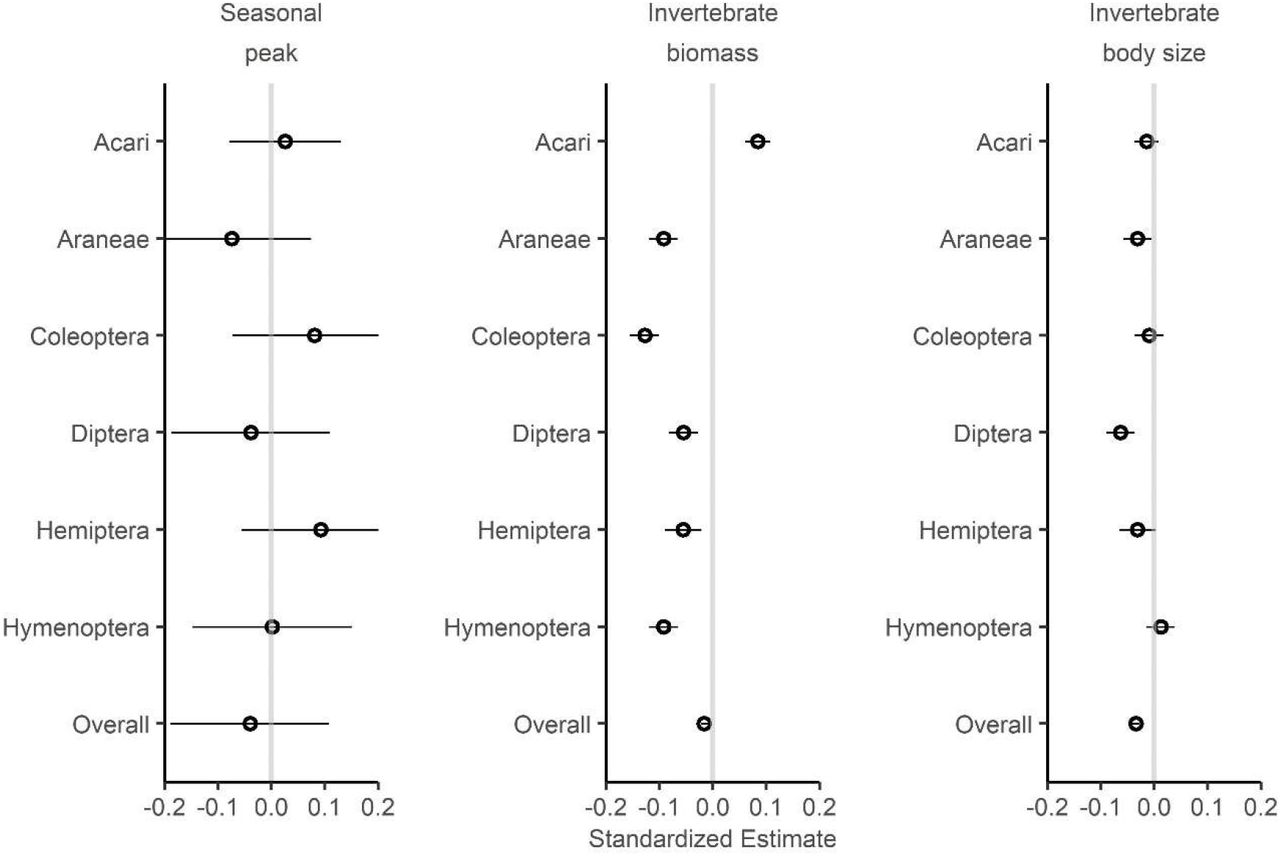
Interannual changes of within season peak timing (left), observed daily invertebrate biomass (center), and median invertebrate body size (right) of six common Orders and the invertebrate assemblage overall. Linear regression estimates are shown as hollow circles, with 95% confidence intervals shown as horizontal lines. Variables with no consistent effect had intervals that crossed zero (grey line).
Chick growth and body condition
We modeled godwit chick growth from 179 mass-at-capture estimates. Chick growth did not differ among years, and our top-performing growth function included both a constant logistic coefficient (K = 0.13 ± 4.2×10⁻³) and inflection point (Ti = 17.5 ± 0.5 days; Supporting information, Table S1).
The fit of our global model was highest with 7-day averaged covariates and no random effects (Supplementary Materials Appendix A, Table S2). Our top model explaining chick BCI (n = 89) included invertebrate biomass and our blocking variable, hatch date, with a smoothed age effect (wi = 0.75; Supplementary Materials Appendix A, Table S3). Chick growth improved with higher invertebrate biomasses (β = 1.8 × 10⁻⁴ ± 3.8 × 10⁻⁵ mg-1, CI: 1.2 × 10⁻⁴, 2.8 × 10⁻⁴; Fig. 4a), but decreased with later hatch dates (β = −0.013 ± 0.003 d-1, CI: −0.0053, −0.019; Fig. 4b). Invertebrate body size had no consistent effect (Supporting information, Fig. S3). Chicks therefore grew as well as or better than expected (e.g., BCI ≥ 1) following weeks with invertebrate biomasses in the upper 15% of those observed or if they hatched before 5 June.

Effect of daily invertebrate biomass (a) and hatch date (b) on godwit chick body condition index (BCI). BCI (hollow points) is the ratio of the observed to expected weight gain since an individual’s last measurement. BCI > 1 correspond with above average growth and BCI < 1 below average growth. Regression line (black) and 95% confidence interval (grey) are shown.
Effect of resources on survival: constant or age-varying?
Of the 128 godwit chicks in our study, we excluded 6 due to human-caused mortality or equipment failure at deployment. The mean DSR of the remaining 122 chicks was 86 ± 24%, meaning that 19.2 ± 33% survived to fledge, although this varied among years and broods (Supporting information, Table S4).
The model with an age-varying effect of invertebrate body size (DIC = 283.0) outperformed the model with an age-varying effect of invertebrate biomass (DIC = 287.9). We therefore used the former in our subsequent tests. The constant effect of invertebrate biomass and the age-varying invertebrate size effect had 79% and 85% posterior inclusion probabilities, respectively (Table 1). We also included constant effects of age and invertebrate size to accompany the interaction term.
Bayesian model selection on variables in a global logistic model predicting daily survival rate in godwit chicks near Beluga River, AK from 2009 – 2019. Predictors were selected using the indicator-variable approach, in which posterior inclusion probabilities (weights) and Bayes Factors (BF) were estimated from a Bernoulli variable associated with each predictor. Variables of the global model with BF > 3 and their component parts (i.e., interaction terms) were included in the top model.
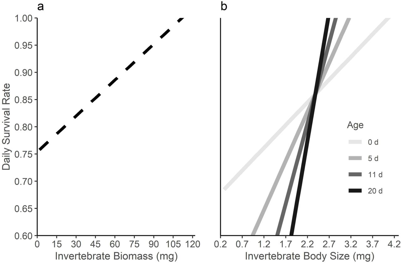
Chick survival improved with higher invertebrate biomasses and larger invertebrate body size, and the latter effect increased throughout development (Table 2). Each 1% increase in daily invertebrate biomass (+ 1.5 mg) improved daily chick survival by 0.66% (Fig. 5a), while each 1% increase in median invertebrate body size (+ 0.06 mg) led to a 1.02% increase in daily chick survival. This ‘size’ effect then grew by 2.2% with each day that a chick survived (Fig. 5b). Age itself, however, had no consistent effect on chick survival.
Standardized effect of variables on the survival rates of godwit chicks near Beluga River, AK from 2009 – 2019. Posterior probabilities were estimated from a hierarchical model (n = 122, posterior samples = 5000) with both survival and stochastic model components.

Effects of daily invertebrate biomass (a) and invertebrate body size (b) on the daily survival of godwit chicks from the posterior mean estimates of a Bayesian hierarchical model (credible intervals not shown). Biomass (dashed) had a constant effect, but the effect of size varied with age (shade of grey, in days).
Population match and reproductive success
The model fit for the whole demand curve (AICc = −300.1) was 25.7-times better than the peak demand curve (AICc = −248.7). Godwits had, on average, 51.9 ± 9.2% overlap with resource phenology according to the peak demand model, but 44.7 ± 11.6% overlap according to the whole demand model. Years also differed in curve height  and the difference between the peak dates of the resource and demand curves
  .
.
Godwit fledging rates varied among study years (Supporting information, Table S5) but were lowest in 2014 and 2015. Models differed in their ability to explain population-level reproductive success but the whole demand model was best supported (Supporting information, Table S6). The whole demand model explained 55% of the variation in godwit fledging rates (β = 1.19 ± 0.41; R2adj. = 0.55; wi = 0.43; Fig. 6a; Supporting information, Fig. S4). The difference in dates model performed similarly well (β = −0.68 ± 0.27; R2adj. = 0.48; wi = 0.36; Fig. 6b) but was 7% less likely to be the top model. Both the curve height (β = 2.49 ± 1.44; R2adj. = 0.25; wi = 0.10; Fig. 6c) and peak demand overlap models (β = 1.00 ± 0.56; R2adj. = 0.26; w, = 0.11; Fig. 6d; Supporting information, Fig. S5) were unlikely to be the top model given their low model weights and the low amounts of interannual variation in fledging rates explained by either.
Correlation of seasonal fledging rates with measures of difference in dates (upper, left), curve height (upper, right), whole demand percent overlap (lower, left), and peak demand percent overlap (lower, right). Yearly fledging rates were extrapolated from daily survival rates with accompanying 95% credible intervals. Regression lines (black) with 95% confidence interval (grey) are shown.
Discussion
The disconnect between empirical studies and the theoretical predictions of the match-mismatch hypothesis casts doubt upon the risks climate change-induced phenological mismatches pose to consumer populations (Visser & Gienapp, 2019; Keogan et al., 2020). To remedy this gap and connect mismatches to demographic processes, Kharouba & Wolkovich (2020) urged researchers to define pre-climate change baselines, collect per-capita data on resources and consumers, and test competing biological mechanisms. We developed mismatch models aimed at fulfilling these recommendations while adopting an ontogenetic view of consumer demand. Using this approach, we built upon the findings of Senner et al. (2017) and identified heretofore undetected individual- and population-level fitness effects of mismatching in the Alaskan breeding population of Hudsonian godwits. Our study joins the growing literature suggesting that mismatches do not fall neatly into a ‘matched’ or ‘mismatched’ paradigm (Keogan et al., 2020; Simmonds et al., 2020). Instead, models built around the underlying biological mechanisms connecting consumers and resources are key to clarifying how mismatching affects consumer fitness (Takimoto & Sato, 2020).
More than mistiming: the tandem drivers of resource availability
We found that resources affected godwit chick survival in two distinct ways: first, periods with reduced resource abundance resulted in poorer growth and lower survival and, second, access to larger invertebrates was increasingly important to the survival of older chicks. Our findings differ from those of previous godwit studies, which found no effects of limited resource availability in the Alaskan godwit breeding population (Senner et al., 2017; Wilde et al., in revision). While these studies did not investigate the influence of invertebrate body size on godwit chicks, our contradictory conclusions likely stem from our use here of hierarchical models that easily approximate time-varying effects on survival (Royle & Dorazio, 2009). Increasing energetic demands throughout ontogeny mean that the effects of resource limitation are unlikely to be constant over an individual’s lifetime (Yang & Rudolf, 2010; Takimoto & Sato, 2020). Therefore, models that accommodate variable predictor effects may be key to clarifying how resource characteristics affect consumer fitness.
Godwit chicks had improved growth and survival following periods with high resource abundance. Having adequate resources during energetically stressful periods is a major driver of animal fitness (Bastille-Rousseau et al., 2015), especially in seasonal environments (McKinnon et al., 2012). Given their high energetic demands and rapid development, chicks of shorebird species across the Arctic have exhibited survival costs following reduced resource abundance (Schekkerman et al., 2003; Saalfeld et al., 2019). Godwit chicks in this study had 3 – 75% higher body condition indices and 17% higher daily survival probabilities, on average, during periods of higher-than-average invertebrate abundance. Importantly, while we also detected effects of hatch date (i.e., phenology) on chick growth, these did not translate into an effect on survival. Our results therefore suggest that relating fitness measures to resource availability captures the effects of mismatching while defining its specific costs in biological terms (Dunn et al., 2011).
In addition to the effects of resource abundance, the quality (i.e., median body size) of invertebrates became increasingly important as godwit chicks aged. Optimal foraging theory predicts that consumers should select resources with the most energy content relative to foraging effort (Krebs et al., 1977). Chicks of black-tailed godwits (Limosa limosa), for instance, prioritize the rapid intake of small prey early in life, but switch to the slower intake of larger prey as they grow older (Schekkerman & Boele, 2009). While we did not observe foraging behaviors directly, we hypothesize that Hudsonian godwit chicks may make a similar transition. In fact, increasing selection of larger prey could explain the especially high costs of poor resource quality for older chicks. We found that periods of below-average prey size resulted in 29% lower survival for chicks below 5-days of age, but 50% lower survival for chicks older than 11-days. Changes in resource quality, though rarely explored in the context of mismatches, can enact strong selection on consumer populations (Keogan et al., 2020; Yang et al., 2020). Because some individuals will encounter high-quality conditions in years when they are ‘mismatched’ (Kerby et al., 2012), accounting for the effects of multiple factors of resource availability could improve our ability to document the true effects of mismatching.
Taken together, the additive effects of resource quantity and quality are likely to worsen in Beluga given the changes we observed in the invertebrate community. Climate-induced reductions in resource availability are common across terrestrial and marine systems (Bowden et al., 2015; Weterings et al., 2018). Arctic invertebrates, in particular, are simultaneously emerging earlier (Høye et al., 2007), becoming less abundant (van Klink et al., 2020), and smaller in size (Bowden et al., 2015; Jonsson et al., 2015) with increasing spring temperatures. Here, we found a linear decrease in the daily abundance (−2%) and body size (−5%) of invertebrates, but no change in the date of peak occurrence of invertebrates over the course of our study. Although we did not detect a linear shift in the timing of the resource peak, this may relate to the occurrence of opposing trends in abundance during the early and late portions of the godwit breeding season. In a post-hoc test, we found that days during the godwit nest incubation period (16 May – 6 June) from 2014 – 2019 had 83% higher invertebrate biomass than those from 2009 – 2012, but 41% lower biomasses on days during the chick-rearing period (6 June – 4 July). Meanwhile, invertebrate body size was 42 – 72% smaller in the later period. Therefore, should these trends continue, developing godwit chicks may face increasingly untenable conditions as food becomes both less abundant and of poorer quality (i.e., smaller size). More broadly, our results suggest that resource timing, quality, and quantity can act as concomitant drivers of phenological mismatches (Rollins & Benard, 2020), and that their effects may be most apparent when placed in the context of the consumer life cycle (Yang et al., 2020).
Modelling the demand-resource interaction clarifies the population effects of mismatching
Variation in godwit reproductive success at the population level was best explained by our whole demand model of mismatching, although the simpler difference in dates model also performed well. Estimates from overlap and dates models do often correlate (Ramakers et al., 2020), but may perform differently depending on a species’ life history and trophic specialization (MillerRushing et al., 2010). Thus, while difference in dates models may suffice for godwits and other species with narrow, synchronous, breeding phenologies or those that rely on singular resource pulses (Miller-Rushing et al., 2010), they would likely perform poorly in species with highly variable nest initiation dates or those capable of multiple nesting events (Phillimore et al., 2016). Because overlap models account for both synchrony and the magnitude of interacting consumerresource pairs, they are more likely to capture mismatching as a disrupted interaction (Kerby et al., 2012). Overlap models are therefore likely more generalizable, but using both overlap and difference in dates models could help when exploring how mismatching occurs on a case-by-case basis (Kellermann & van Riper, 2015).
Not all overlap models are equivalent, however. Overlap models have received mixed support (Ramakers et al., 2020), but their ability to accurately quantify mismatching at the tails of the consumer curve has been suggested as an important component of their effectiveness (Kerby et al., 2012). Accordingly, whereas our peak demand model performed relatively poorly and explained only 21% variation in godwit reproductive success, our whole demand model had 25-fold better model fit than the peak demand model and explained 55% of the variation in fledging rates. This difference likely stems from the inability of the peak demand model to accurately capture consumer demand at the upper (i.e., right-hand) tail of the consumer curve, corresponding to the period when individual-level consumer demand is greatest. Our results therefore show that incorporating additional nuance into the statistical concept of consumer phenologies can greatly improve overlap models (Lindén, 2018).
The need to accurately identify mismatches is made most clear by the accumulating evidence for variable and non-linear responses by consumer populations to mismatching (Visser & Both, 2005; Phillimore et al., 2016). So called ‘tipping points’ – thresholds past which an effect abruptly changes (Latty & Dakos, 2019) – buffer consumer populations from the negative impacts of moderate mismatching and may contribute to the lack of consistent responses to mismatching across consumer populations (Simmonds et al., 2020). In godwits, we found that greater population-level mismatching consistently drove poorer fledging success, but that there may be thresholds past which the effects are most severe. For instance, godwits experienced ~19% poorer overlap and ~28 days greater mismatching in 2014 and 2015 compared to the longterm average. Mismatching on this scale resulted in 24% lower fledging rates and near complete reproductive failure for the population. Similarly low fledging rates for Hudson Bay breeding godwits, which are mismatched by 11-days on-average (Senner et al., 2017), suggests that for godwits, this tipping point may exist when populations are mismatched by more than ~10 days or have less than 40% overlap with the resource curve.
Importantly, though, the 2014 and 2015 seasons in Beluga coincided with a period of anomalous and prolonged near-surface warming in the northeastern Pacific called the ‘blob’ (Cavole et al., 2016). Thus, while the conditions in these atypical years may provide useful insights into potential outcomes of a warming climate on coastal communities in the region (Auth et al., 2018), mismatches of this magnitude are unlikely to become the norm. Beluga godwits have been able to advance their timing of migration and reproduction in response to recent long-term, linear, warming trends (Senner 2012; Senner et al., 2017) and may therefore be able to do so in the future. Nonetheless, significant spring warming and earlier snow disappearance dates projected for the North American sub-Arctic mean that godwits and other migratory populations may soon face accelerating, potentially non-linear, warming (Littell et al., 2018; Lader et al., 2020). Quantifying the strength and effects of mismatching in real time will thus be crucial for conservation going forward (Simmonds et al., 2020).
Conclusions
By modelling the unspoken assumptions of the match-mismatch hypothesis, we stand to adopt a more powerful definition of mismatching in biological terms and, in so doing, be better able to identify the circumstances under which consumer populations perform poorly. Our work also illustrates the role of ontogeny in shaping an individual’s changing response to resource availability over time (Yang & Rudolf, 2010), and helps explain the empirical-theoretical disconnect in phenological studies. Importantly, our models are transferrable to other systems, whereby remotely sensed indices and knowledge of a population’s age-structure could approximate resource availability and metabolic rate, respectively, when these data are otherwise unavailable (Lumbierres et al., 2017). Finally, we show how treating mismatches as an outcome of both demand and resource dynamics provides insight into the structure of individual-level effects and the mechanism behind population-level responses (Takimoto & Sato, 2020). Replacing the categorical ‘matched or mismatched’ view of mismatching with one that explicitly recognizes the underlying mechanism may be critical to monitoring and conserving animal populations in an uncertain future.
Author Contributions
LRW and NRS conceived of the study. All authors collected field data. LRW analyzed the data and wrote the manuscript. All authors contributed to revisions.
Data Availability Statement
Data are deposited at Dryad (https://doi.org/10.5061/dryad.x69p8czh0) and computer code for all analyses are available at github (http://doi.org/10.5281/zenodo.4298755).
Acknowledgements
We thank the Cook Inlet Region Inc. for permitting us access to their lands. We thank Drs. Sarah Converse and Emily Weiser for analytical guidance. Funding was provided by the Association of Field Ornithologists, Wilson Ornithological Society, American Ornithological Society, Arctic Audubon Society, Cornell Lab of Ornithology, Athena Fund at the Cornell Lab of Ornithology, University of South Carolina, Faucett Family Foundation, the David and Lucile Packard Foundation, National Science Foundation (PCE-1110444 and DGE-1144153), and the U.S. Fish and Wildlife Service (4074, 5147). All procedures met the ethical standards of the University of South Carolina (2449-101417-042219), Alaska Department of Fish and Game (20-024), and USGS (24191). Any use of trade, product, or firm names is for descriptive purposes only and does not imply endorsement by the U.S. Government. The authors declare no conflict of interest.
References


